Asymptotic Regional Boundary Observer in Distributed Parameter Systems via Sensors Structures

Abstract
:1. Introduction
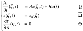
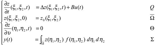
2. Problem Statement

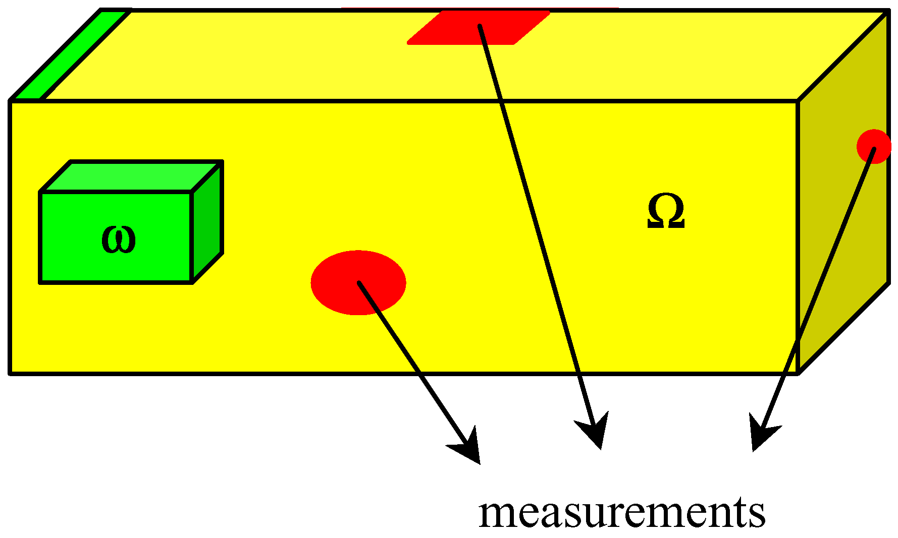
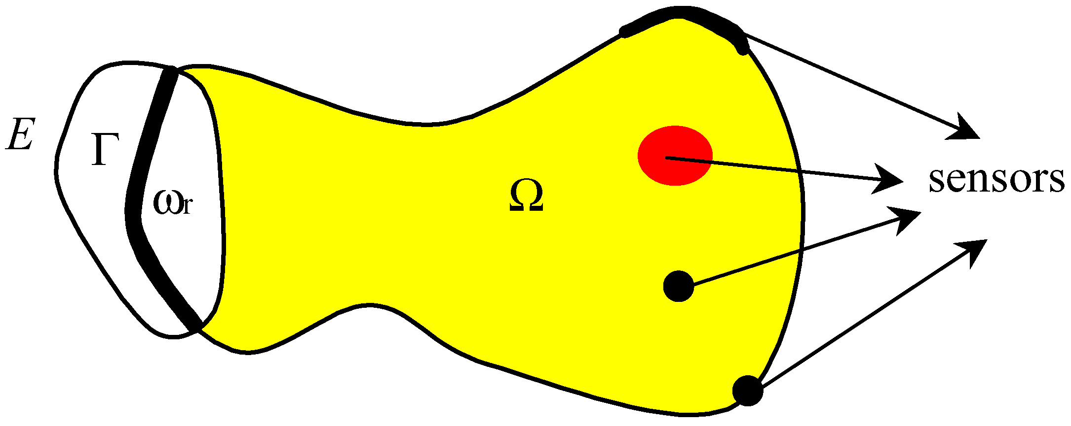
- Let us recall that a sensor by any couple (D, f) where D denote closed subsets of , which is spatial support of sensor and f ∈ L2 (D) defines the spatial distribution of measurement on D. According to the choice of the parameters D and f, we have various types of sensors. A sensors may be a zone types when D ⊂ Ω. The output function (2.2) can be written in the formy (t) = Cz(., t) = ∫D z(ξ, t) f (ξ)dξ


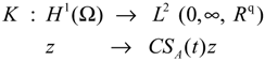
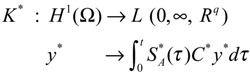
- The operator K defined byand in the case of internal zone sensors is, linear and bounded with an adjoint
![Sensors 02 00137 i005]()
![Sensors 02 00137 i052]()
- The trace operator of order zerois linear, surjective and continuous with adjoint denoted by γ0*
![Sensors 02 00137 i006]()
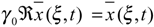
- Consider a subdomain Γ of ∂Ω and let χΓ be the function defined bywhere z|Γ is the restriction of the state z to Γ. We denote by the adjoint of χΓ.
![Sensors 02 00137 i007]()
- Let χω be the function defined bywhere z|Γ is the restriction of the state z to ω.
![Sensors 02 00137 i008]()
- The operator TΓ : H1(Ω) → H1/2(Γ) is given by
![Sensors 02 00137 i009]()


- The autonomous system associated to (2.1)-(2.2) is said to be exactly (respectively weakly) Γ-observable if :
![Sensors 02 00137 i010]()
- The suite (Di, fi)1≤i≤q of sensors is said to be Γ-strategic if the system (2.1) together with the output function (2.2) is weakly Γ-observable. For the dual results concerning the actuators structures [17].

3. Regional boundary detectability
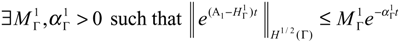
- The system (2.1) is said to be ∂Ω-stable, if the operator A generates a semi-group which is stable on the space H1/2 (∂Ω). It is easy to see that the system (2.1) is ∂Ω-stable, if and only if, for some positive constants M and α, we have
![Sensors 02 00137 i011]()

- The system (2.1) together with the output (2.2) is said to be ∂Ω-detectable, if there exists an operator H∂Ω: Rq → H1/2(∂Ω) such that (A – H∂ΩC) generates a strongly continuous semi-group (SH∂Ω (t))t≥0 which is stable on H1/2 (∂Ω).
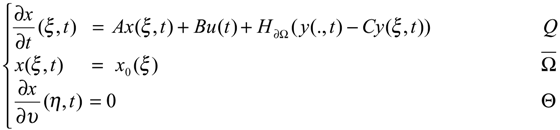
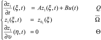
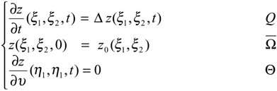
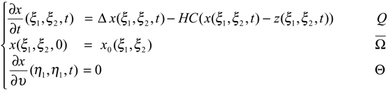
- If a system is ∂Ω-detectable, then it is possible to construct an asymptotic ∂Ω-observer for the original system. If we consider the system
![Sensors 02 00137 i013]()

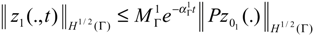
- The system (2.1) is said to be Γ-stable, if the operator A generates a semi-group which is stable on H1/2 (Γ).
- The system (2.1)-(2.2) is said to be Γ-detectable if there exists an operator HΓ: Rq → H1/2(Γ) such that (A − HΓC) generates a strongly continuous semi-group (SHΓ(t))t≥0 which is stable on H1/2 (Γ).

4. Asymptotic Γ-observer and strategic sensors
4.1. Definitions and characterizations
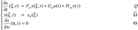
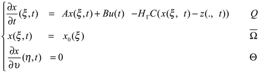
- Consider the system (2.1) - (2.2) together with the dynamical systemwhere Fω generates a strongly continuous semi-group (SFω(t))t≥0 which is stable on X = H1 (ω), i.e. :
![Sensors 02 00137 i016]() and Gω∈L(Rp, H1 (ω)) and Hω ∈L(Rq, H1 (ω)). The system (4.1) defines an asymptotic ω-estimator for χωT(ξ,t) where z(ξ,t) is a solution of the system (2.1) - (2.2) if and χωT maps D(A) into D(Fω) where x(ξ, t) is the solution of the system (4.1).
and Gω∈L(Rp, H1 (ω)) and Hω ∈L(Rq, H1 (ω)). The system (4.1) defines an asymptotic ω-estimator for χωT(ξ,t) where z(ξ,t) is a solution of the system (2.1) - (2.2) if and χωT maps D(A) into D(Fω) where x(ξ, t) is the solution of the system (4.1).![Sensors 02 00137 i017]()
- The system (4.1) specifies an ω-observer for the system (2.1) - (2.2) if the following conditions hold:
- There exists Mω ∈ L(Rq, L2 (ω)) and Nω ∈ L(L2 (ω)) such that MωC + NωχωT = Iω.
- χωTA + FωχωT = GωC and Hω=χωTB.
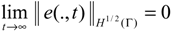
- The system (4.1) defines an asymptotic ω-estimator for χωT (ξ,t).
- The system (4.1) is said to be an identity ω-observer for the system (2.1) - (2.2) if and Z = X.
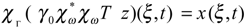
- The boundary regional observer in Γ may be seen as internal regional observer in ω if we consider the following transformations. Let ℜ be the continuous linear extension operator [19] ℜ: H1/2 (∂ Ω) → H1 (Ω) such that
![Sensors 02 00137 i018]()
- Let r>0 is an arbitrary and sufficiently small real and let the setswhere B(z, r) is the ball of radius r centered in z(ξ,t) and where Γ is a part of (Fig. 2).
![Sensors 02 00137 i019]()


4.2 Sufficient condition for Γ-observer
- q > s
- rank Gn = rn, ∀n, n = 1,..., J withwhere sup sn = s < ∞ and j = 1,..., sn. Then the dynamical system
![Sensors 02 00137 i025]() is Γ-observer for the system (2.1) - (2.2), i.e. .
is Γ-observer for the system (2.1) - (2.2), i.e. .![Sensors 02 00137 i026]()


- A dynamical system which is an ∂Ω -observer is Γ-observer.
- If a system is Γ-observer, then it is Γ1 -observer in every subset Γ1 of Γ, but the converse is not true. This may be proven in the following example:

5. Application to sensors structures
5.1 Case of a zone sensor
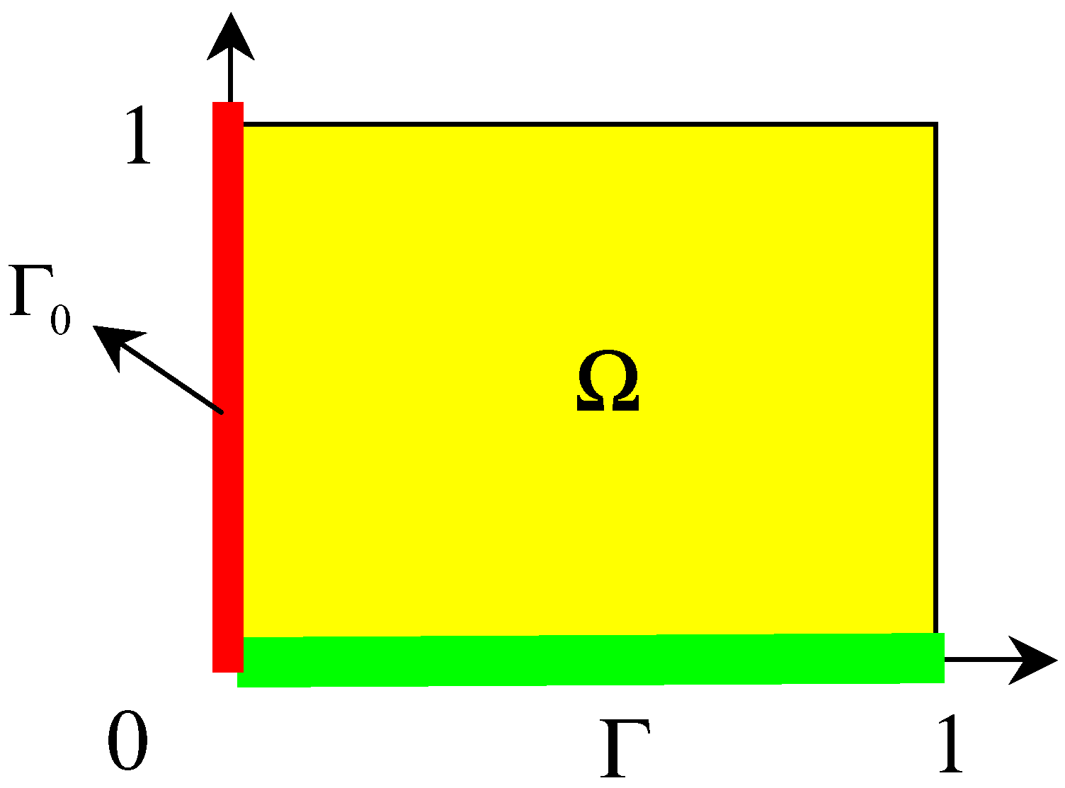
5.1.1 Rectangular domain


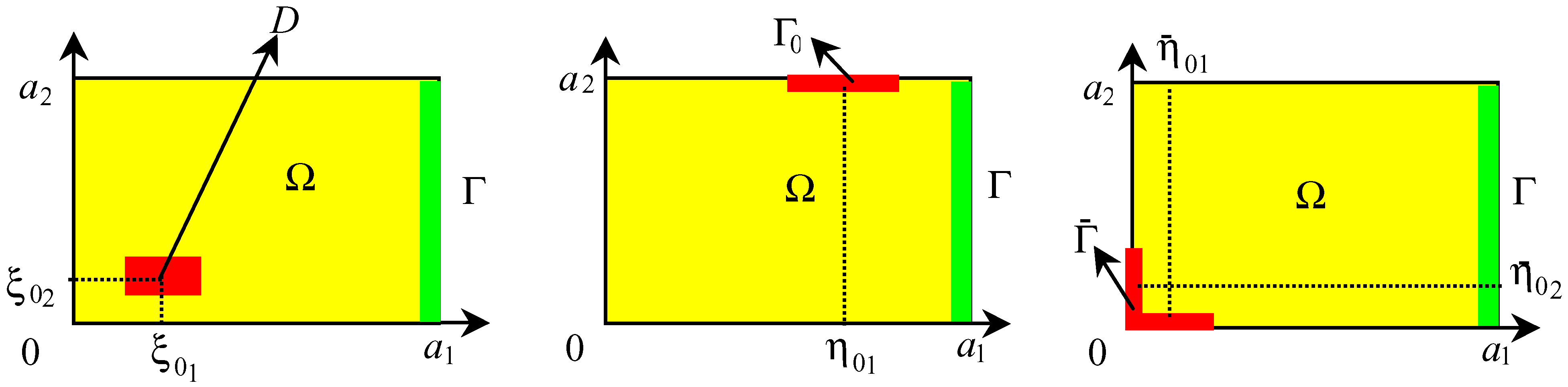
- One side case : Suppose that the sensor (D, f) is located on Γ0 =[η01 − l, η01 + l] × { a2 } ⊂ ∂Ω and f is symmetric with respect to η1 = η01, then the dynamical system (5.4) is Γ-observer for the system (5.1) if n η01 / a1 ∉N for every n, m =1,..., J.
- Two side case : Suppose that the sensor (D, f) is located on and is symmetric with respect to η1 = η01 and the function is symmetric with respect to η2 = η02, then the dynamical system (5.4) is Γ-observer for the system (5.1) if n η01 / a1 and mη02 / a2 ∉N for every n, m = 1,..., J.
5.1.2 Disk domain


5.2 Case a pointwise sensor
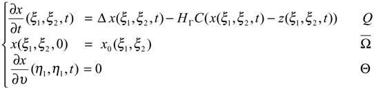
5.2.1 The domain Ω =]0,a1[×]0,a2[
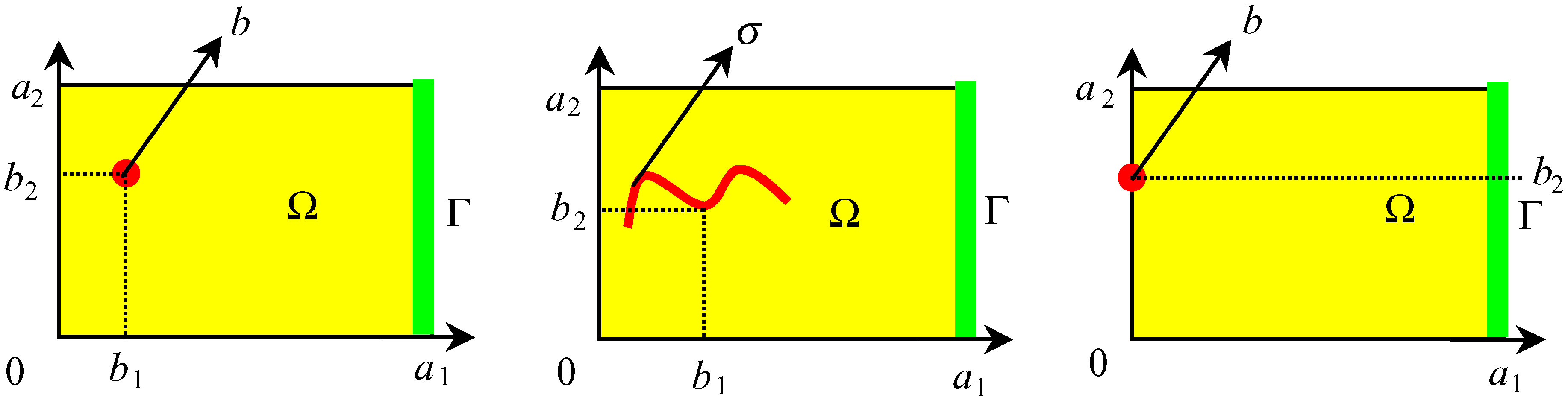
- Internal case : If nb1 / a1 and mb2 / a2 ∉N for every n, m = 1,..., J, then the dynamical system (5.4) is Γ-observer for the system (5.9).
- Filament case : Suppose that the observation is given by the filament sensor where σ = Im(γ) is symmetric with respect to the line b = (b1,b2), if nb1 / a1 and mb2 / a2 ∉N for every n, m = 1,..., J, the dynamical system (5.4) is Γ-observer for the system (5.9).
- Boundary case : If mb2 / a2 ∉N for every m = 1,..., J, then the dynamical system (5.4) is Γ- observer for the system (5.9).
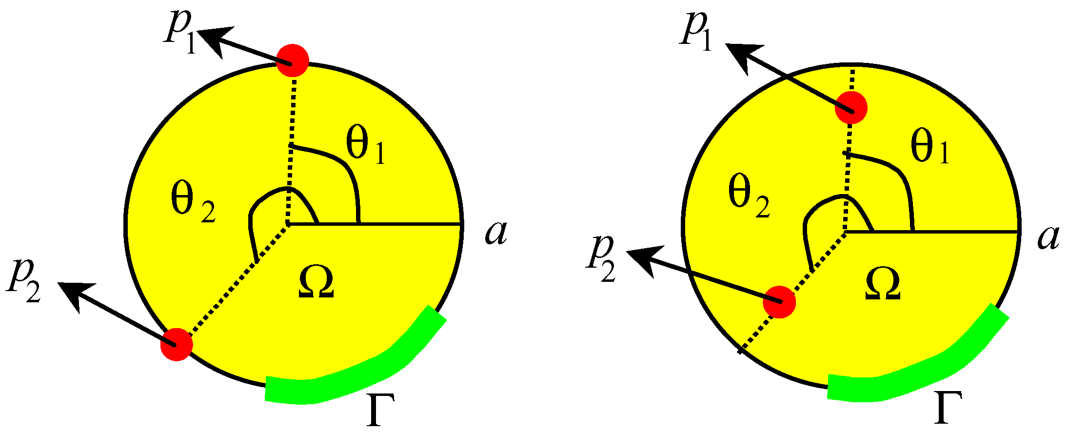
5.2.2 The domain Ω = D(0,a)

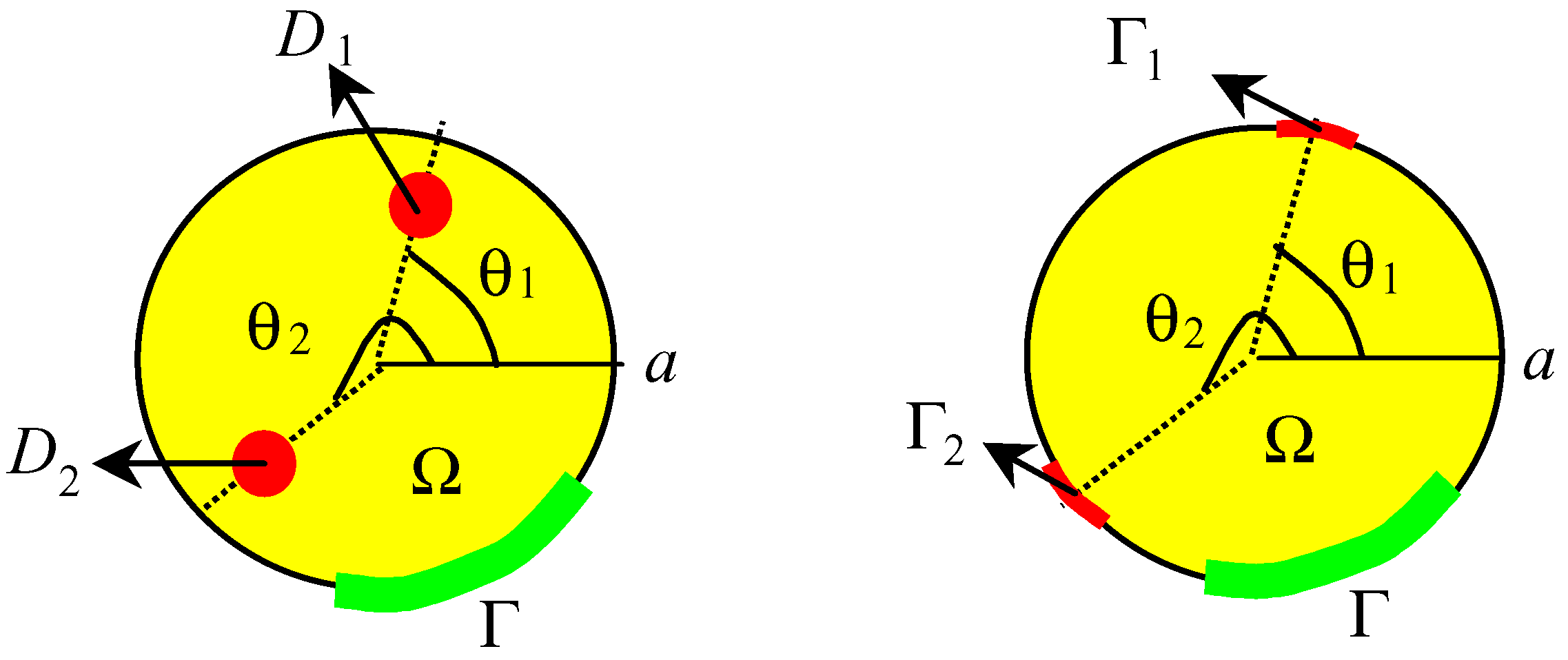
- If the sensors (pi,δpi)2≤i≤q are located in pi =(ri,θi) and n(θ1 − θ2)/π ∉ N for every n, n =1,..., J, then the dynamical system (5.8) is Γ-observer for the system (5.10).
- If the sensors (pi,δpi) are located in pi =(a,θi) 2≤i≤q and n(θ1 − θ2)/π ∉ N for every n, n =1,..., J, then the dynamical system (5.8) is Γ-observer for the system (5.10).
6. Conclusion
References
- Luenberger, D. Observers for multi-variable systems. IEEE Transactions on Automatics Control 1966, 11, 190–197. [Google Scholar] [CrossRef]
- Gressang, R.; Lamont, G. B. Observers for systems characterized by semi-groups. IEEE Transactions on Automatics Control 1975, 20, 523–528. [Google Scholar] [CrossRef]
- Fujii, N.; Hirai, M. A finite-dimensional asymptotic observer for a class of distributed parameter systems. International Journal of Control 1980, 32, 951–961. [Google Scholar] [CrossRef]
- Hou, M.; Muller, P.C. Design of observers for linear systems with unknown inputs. IEEE Transactions Automatic Control 1992, 37, 871–875. [Google Scholar] [CrossRef]
- Curtain, R. F.; Zwart, H. J. Introduction to infinite dimensional linear theory systems; Springer-Verlag: New York, 1995. [Google Scholar]
- El Jai, A.; Pritchard, A. J. Sensors and actuators in distributed parameter systems. International Journal of Control 1987, 46, 1139–1153. [Google Scholar] [CrossRef]
- El Jai, A.; Pritchard, A. J. Sensors and controls in the analysis of distributed systems; Ellis Horwood series in Mathematics and its Applications; Wiley: New York, 1988. [Google Scholar]
- El Jai, A.; Simon, M. C.; Zerrik, E. Regional observability and sensor structures. Sensors and Actuators 1993, 39, 95–102. [Google Scholar] [CrossRef]
- Zerrik, E.; Badraoui, L.; El Jai, A. Sensors and regional boundary state reconstruction of parabolic systems. Sensors and Actuators 1999, 75, 102–117. [Google Scholar] [CrossRef]
- El Jai, A.; Zerrik, E.; Simon, M. C.; Amouroux, M. Regional observability of a thermal process. IEEE Transactions on Automatic Control 1995, 40, 518–521. [Google Scholar] [CrossRef]
- Al-Saphory, R.; El Jai, A. Sensors and asymptotic ω-observer for distributed diffusion systems. Sensors 2001, 1, 161–182. [Google Scholar] [CrossRef]
- Al-Saphory, R.; El Jai, A. Sensors structures and regional detectability of parabolic distributed systems. Sensors and Actuators 2001, 29, 163–171. [Google Scholar] [CrossRef]
- Al-Saphory, R.; El Jai, A. Sensors characterizations for regional boundary detectability of distributed parameter systems. Sensors and Actuators 2001, 94, 1–10. [Google Scholar] [CrossRef]
- Al-Saphory, R.; El Jai, A. Asymptotic regional state reconstruction. International Journal of Systems Science 2002. to appear. [Google Scholar] [CrossRef]
- Curtain, R. F. Finite dimensional compensators for parabolic distributed systems with unbounded control and observation. SIAM J. Control and Optimisation 1984, 22, 255–275. [Google Scholar] [CrossRef]
- Zerrik, E.; Badraoui, L. Sensors characterization for regional boundary observability. International Journal of Applied Mathematics and Computer Science 2000, 10, 345–356. [Google Scholar]
- Zerrik, E.; Boutoulout, L.; El Jai, A. Actuators and regional boundary controllability of parabolic systems. International Journal of Systems Science 2000, 31, 73–82. [Google Scholar] [CrossRef]
- Al-Saphory, R. Asymptotic regional analysis for a class of distributed parameter systemes. Ph.D. thesis, University of Perpignan, France, 2001. [Google Scholar]
- Dautray, R.; Lions, J.L. Analyse mathématique et calcul numérique pour les sciences et les techniques; série scientifique 8; Masson: Paris, 1984. [Google Scholar]
- Kitamura, S.; Sakairi, S.; Nishimura, M. Observer for distributed-parameter diffusion systems. Electrical engineering in Japan 1972, 92, 142–149. [Google Scholar] [CrossRef]
- El Jai, A.; El Yacoubi, S. On the number of actuators in parabolic system. International Journal of Applied Mathematics and Computer Science 1993, 3, 673–686. [Google Scholar]
- Sample Availability: Available from the authors.
© 2002 by MDPI (http://www.mdpi.net). Reproduction is permitted for noncommercial purposes.
Share and Cite
Al-Saphory, R. Asymptotic Regional Boundary Observer in Distributed Parameter Systems via Sensors Structures. Sensors 2002, 2, 137-152. https://doi.org/10.3390/s20400137
Al-Saphory R. Asymptotic Regional Boundary Observer in Distributed Parameter Systems via Sensors Structures. Sensors. 2002; 2(4):137-152. https://doi.org/10.3390/s20400137
Chicago/Turabian StyleAl-Saphory, Raheam. 2002. "Asymptotic Regional Boundary Observer in Distributed Parameter Systems via Sensors Structures" Sensors 2, no. 4: 137-152. https://doi.org/10.3390/s20400137
APA StyleAl-Saphory, R. (2002). Asymptotic Regional Boundary Observer in Distributed Parameter Systems via Sensors Structures. Sensors, 2(4), 137-152. https://doi.org/10.3390/s20400137