Separating Leaf and Wood Points in Terrestrial Laser Scanning Data Using Multiple Optimal Scales


Abstract
1. Introduction
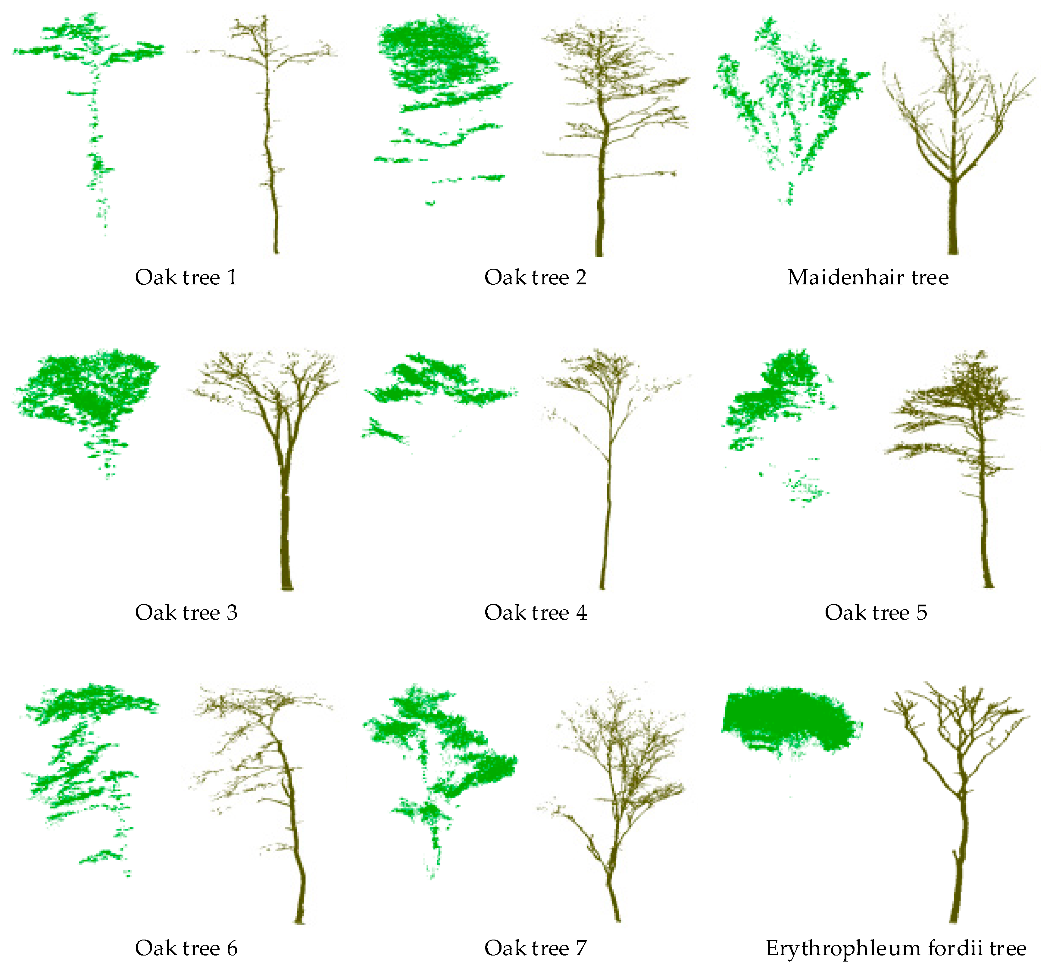
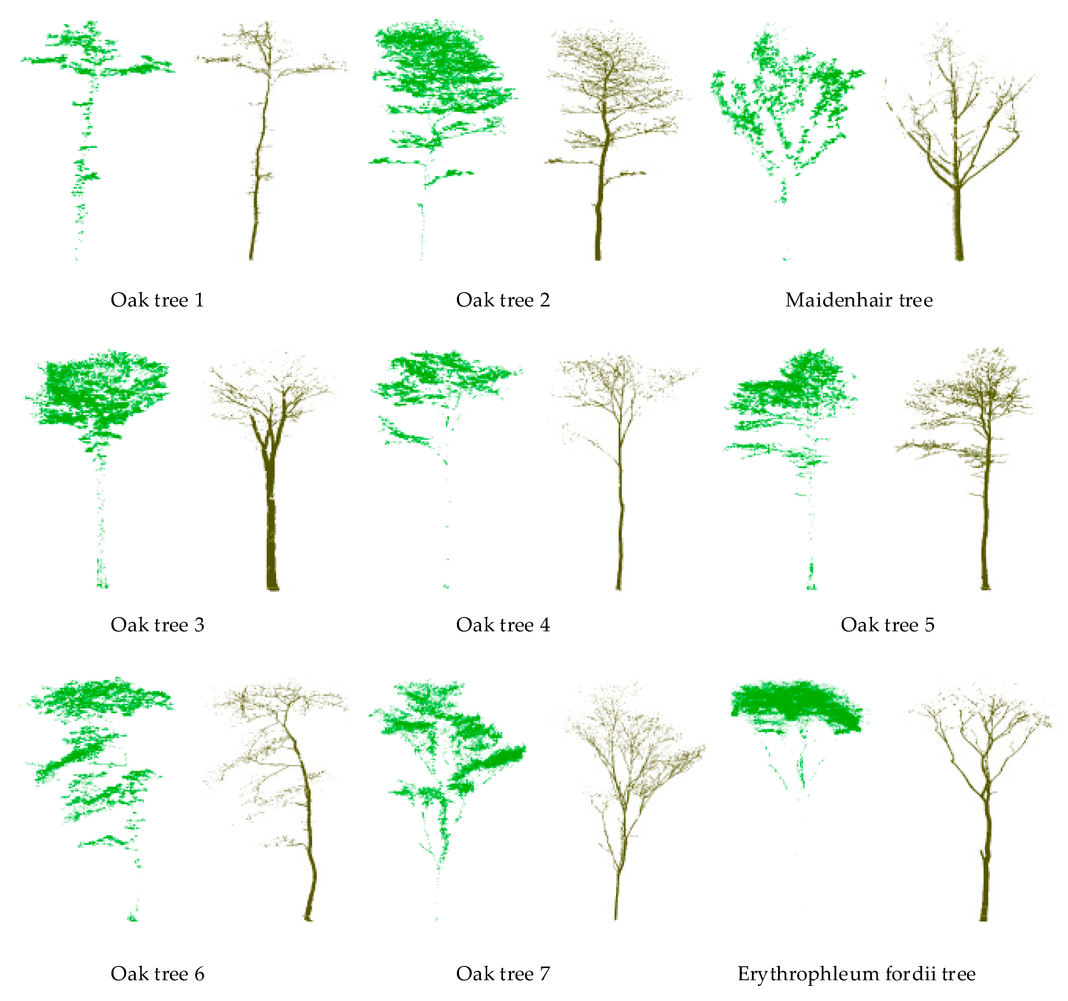
2. Experimental Data
3. Methods.
3.1. Scale Definition and Selection of Multiple Optimal Scales
3.2. Features Extraction
3.3. Separation Method
3.4. Optimization Strategy
3.5. Evaluation
4. Experimental Results and Discussion
5. Conclusions
Author Contributions
Funding
Acknowledgments
Conflicts of Interest
References
- Dassot, M.; Constant, T.; Fournier, M. The use of terrestrial LiDAR technology in forest science: Application fields, benefits and challenges. Ann. For. Sci. 2011, 68, 959–974. [Google Scholar] [CrossRef]
- Ma, Y.; Piao, S.; Sun, Z.; Lin, X.; Wang, T.; Yue, C.; Yang, Y. Stand ages regulate the response of soil respiration to temperature in a Larix principis-rupprechtii plantation. Agric. For. Meteorol. 2014, 184, 179–187. [Google Scholar] [CrossRef]
- Srinivasan, S.; Popescu, S.C.; Eriksson, M.; Sheridan, R.D.; Ku, N.-W. Multi-temporal terrestrial laser scanning for modeling tree biomass change. For. Ecol. Manag. 2014, 318, 304–317. [Google Scholar] [CrossRef]
- Sun, Z.; Liu, L.; Peng, S.; Peñuelas, J.; Zeng, H.; Piao, S. Age-related modulation of the nitrogen resorption efficiency response to growth requirements and soil nitrogen availability in a temperate pine plantation. Ecosystems 2016, 19, 698–709. [Google Scholar] [CrossRef]
- Liang, X.; Kankare, V.; Hyyppä, J.; Wang, Y.; Kukko, A.; Haggrén, H.; Yu, X.; Kaartinen, H.; Jaakkola, A.; Guan, F.; et al. Terrestrial laser scanning in forest inventories. ISPRS-J. Photogramm. Remote Sens. 2016, 115, 63–77. [Google Scholar] [CrossRef]
- Hackenberg, J.; Wassenberg, M.; Spiecker, H.; Sun, D. Non destructive method for biomass prediction combining TLS derived tree volume and wood density. Forests 2015, 6, 1274–1300. [Google Scholar] [CrossRef]
- Tao, S.; Guo, Q.; Xu, S.; Su, Y.; Li, Y.; Wu, F. A geometric method for wood-leaf separation using terrestrial and simulated LiDAR data. Photogramm. Eng. Remote Sens. 2015, 81, 767–776. [Google Scholar] [CrossRef]
- Delagrange, S.; Jauvin, C.; Rochon, P. PypeTree: A tool for reconstructing tree perennial tissues from point clouds. Sensors 2014, 14, 4271–4289. [Google Scholar] [CrossRef] [PubMed]
- Dassot, M.; Colin, A.; Santenoise, P.; Fournier, M.; Constant, T. Terrestrial laser scanning for measuring the solid wood volume, including branches, of adult standing trees in the forest environment. Comput. Electron. Agric. 2012, 89, 86–93. [Google Scholar] [CrossRef]
- Hackenberg, J.; Spiecker, H.; Calders, K.; Disney, M.; Raumonen, P. SimpleTree—An efficient open source tool to build tree models from TLS clouds. Forests 2015, 6, 4245–4294. [Google Scholar] [CrossRef]
- Zheng, G.; Moskal, L.M.; Kim, S.-H. Retrieval of effective leaf area index in heterogeneous forests with terrestrial laser scanning. IEEE Trans. Geosci. Remote Sens. 2013, 51, 777–786. [Google Scholar] [CrossRef]
- Wei, H.; Zhou, G.; Zhou, J. Comparison of single and multi-scale method for leaf and wood points classification from terrestrial laser scanning data. In Proceedings of the ISPRS Annals of the Photogrammetry, Remote Sensing and Spatial Information Sciences, Beijing, China, 7–10 May 2018; pp. 217–223. [Google Scholar]
- Béland, M.; Baldocchi, D.D.; Widlowski, J.-L.; Fournier, R.A.; Verstraete, M.M. On seeing the wood from the leaves and the role of voxel size in determining leaf area distribution of forests with terrestrial LiDAR. Agric. For. Meteorol. 2014, 184, 82–97. [Google Scholar] [CrossRef]
- Ma, L.; Zheng, G.; Eitel, J.U.H.; Moskal, L.M.; He, W.; Huang, H. Improved salient feature-based approach for automatically separating photosynthetic and nonphotosynthetic components within terrestrial LiDAR point cloud data of forest canopies. IEEE Trans. Geosci. Remote Sens. 2016, 54, 679–696. [Google Scholar] [CrossRef]
- Wang, D.; Brunner, J.; Ma, Z.; Lu, H.; Hollaus, M.; Pang, Y.; Pfeifer, N. Separating tree photosynthetic and non-photosynthetic components from point cloud data using dynamic segment merging. Forests 2018, 9, 252. [Google Scholar] [CrossRef]
- Wang, D.; Hollaus, M.; Pfeifer, N. Feasibility of machine learning methods for separating wood and leaf points from terrestrial laser scanning data. In Proceedings of the ISPRS Annals of Photogrammetry, Remote Sensing and Spatial Information Sciences, Wuhan, China, 18–22 September 2017; pp. 157–164. [Google Scholar]
- Béland, M.; Widlowski, J.-L.; Fournier, R.A.; Côté, J.-F.; Verstraete, M.M. Estimating leaf area distribution in savanna trees from terrestrial LiDAR measurements. Agric. For. Meteorol. 2011, 151, 1252–1266. [Google Scholar] [CrossRef]
- Hakala, T.; Suomalainen, J.; Kaasalainen, S.; Chen, Y. Full waveform hyperspectral LiDAR for terrestrial laser scanning. Opt. Express 2012, 20, 7119. [Google Scholar] [CrossRef]
- Belton, D.; Moncrieff, S.; Chapman, J. Processing tree point clouds using Gaussian Mixture Models. In Proceedings of the ISPRS Annals of Photogrammetry, Remote Sensing and Spatial Information Sciences, Antalya, Turkey, 11–13 November 2013; pp. 43–48. [Google Scholar]
- Li, S.; Dai, L.; Wang, H.; Wang, Y.; He, Z.; Lin, S. Estimating leaf area density of individual trees using the point cloud segmentation of terrestrial LiDAR data and a voxel-based model. Remote Sens. 2017, 9, 1202. [Google Scholar] [CrossRef]
- Ioannou, Y.; Taati, B.; Harrap, R.; Greenspan, M. Difference of normals as a multi-scale operator in unorganized point clouds. In Proceedings of the 2012 Second International Conference on 3D Imaging, Modeling, Processing, Visualization & Transmission, Zurich, Switzerland, 13–15 October 2012; pp. 501–508. [Google Scholar]
- Ferrara, R.; Virdis, S.G.P.; Ventura, A.; Ghisu, T.; Duce, P.; Pellizzaro, G. An automated approach for wood-leaf separation from terrestrial LiDAR point clouds using the density based clustering algorithm DBSCAN. Agric. For. Meteorol. 2018, 262, 434–444. [Google Scholar] [CrossRef]
- Xu, S.; Xu, S.; Ye, N.; Zhu, F. Automatic extraction of street trees’ nonphotosynthetic components from MLS data. Int. J. Appl. Earth Obs. Geoinf. 2018, 69, 64–77. [Google Scholar] [CrossRef]
- Yun, T.; An, F.; Li, W.; Sun, Y.; Cao, L.; Xue, L. A novel approach for retrieving tree leaf area from ground-based LiDAR. Remote Sens. 2016, 8, 942. [Google Scholar] [CrossRef]
- Li, Z.; Schaefer, M.; Strahler, A.; Schaaf, C.; Jupp, D. On the utilization of novel spectral laser scanning for three-dimensional classification of vegetation elements. Interface Focus 2018, 8, 20170039. [Google Scholar] [CrossRef] [PubMed]
- Zhu, X.; Skidmore, A.K.; Darvishzadeh, R.; Niemann, K.O.; Liu, J.; Shi, Y.; Wang, T. Foliar and woody materials discriminated using terrestrial LiDAR in a mixed natural forest. Int. J. Appl. Earth Obs. Geoinf. 2018, 64, 43–50. [Google Scholar] [CrossRef]
- Calders, K.; Disney, M.I.; Armston, J.; Burt, A.; Brede, B.; Origo, N.; Muir, J.; Nightingale, J. Evaluation of the range accuracy and the radiometric calibration of multiple terrestrial laser scanning instruments for data interoperability. IEEE Trans. Geosci. Remote Sens. 2017, 55, 2716–2724. [Google Scholar] [CrossRef]
- Kaasalainen, S.; Jaakkola, A.; Kaasalainen, M.; Krooks, A.; Kukko, A. Analysis of incidence angle and distance effects on terrestrial laser scanner intensity: Search for correction methods. Remote Sens. 2011, 3, 2207–2221. [Google Scholar] [CrossRef]
- Brodu, N.; Lague, D. 3D terrestrial LiDAR data classification of complex natural scenes using a multi-scale dimensionality criterion: Applications in geomorphology. ISPRS-J. Photogramm. Remote Sens. 2012, 68, 121–134. [Google Scholar] [CrossRef]
- Lalonde, J.-F.; Vandapel, N.; Huber, D.F.; Hebert, M. Natural terrain classification using three-dimensional ladar data for ground robot mobility. J. Field Robot. 2006, 23, 839–861. [Google Scholar] [CrossRef]
- Weinmann, M.; Jutzi, B.; Hinz, S.; Mallet, C. Semantic point cloud interpretation based on optimal neighborhoods, relevant features and efficient classifiers. ISPRS-J. Photogramm. Remote Sens. 2015, 105, 286–304. [Google Scholar] [CrossRef]
- Weinmann, M.; Urban, S.; Hinz, S.; Jutzi, B.; Mallet, C. Distinctive 2D and 3D features for automated large-scale scene analysis in urban areas. Comput. Graph. 2015, 49, 47–57. [Google Scholar] [CrossRef]
- Weinmann, M.; Weinmann, M.; Mallet, C.; Brédif, M. A classification-segmentation framework for the detection of individual trees in dense mms point cloud data acquired in urban areas. Remote Sens. 2017, 9, 277. [Google Scholar] [CrossRef]
- Demantké, J.; Mallet, C.; David, N.; Vallet, B. Dimensionality based scale selection in 3D LiDAR point clouds. In Proceedings of the ISPRS—International Archives of the Photogrammetry, Remote Sensing and Spatial Information Sciences, Calgary, Canda, 29–31 August 2011; pp. 97–102. [Google Scholar]
- Lalonde, J.; Unnikrishnan, R.; Vandapel, N.; Hebert, M. Scale selection for classification of point-sampled 3D surfaces. In Proceedings of the Fifth International Conference on 3-D Digital Imaging and Modeling (3DIM’05), Ottawa, ON, Canada, 13–16 June 2005; pp. 285–292. [Google Scholar]
- Wang, Z.; Zhang, L.; Fang, T.; Mathiopoulos, P.T.; Tong, X.; Qu, H.; Xiao, Z.; Li, F.; Chen, D. A multiscale and hierarchical feature extraction method for terrestrial laser scanning point cloud classification. IEEE Trans. Geosci. Remote Sens. 2015, 53, 2409–2425. [Google Scholar] [CrossRef]
- Jolliffe, I.T. Principal Component Analysis, 2nd ed.; Springer: Berlin, Germany, 2002. [Google Scholar]
- Shannon, C.E. A mathematical theory of communication. Bell Syst. Tech. J. 1948, 27, 379–423. [Google Scholar] [CrossRef]
- Breiman, L. Random forests. Mach. Learn. 2001, 45, 5–32. [Google Scholar] [CrossRef]
- Weinmann, M.; Jutzi, B.; Mallet, C. Semantic 3D scene interpretation: A framework combining optimal neighborhood size selection with relevant features. In Proceedings of the ISPRS Annals of Photogrammetry, Remote Sensing and Spatial Information Sciences, Zurich, Switzerland, 5–7 September 2014; pp. 181–188. [Google Scholar]
- Sanna, K.; Anssi, K.; Jari, L.; Pasi, R.; Harri, K.; Mikko, K.; Eetu, P.; Kati, A.; Raisa, M. Change detection of tree biomass with terrestrial laser scanning and quantitative structure modelling. Remote Sens. 2014, 6, 3906–3922. [Google Scholar]


| Trees | Leaf Points | Wood Points | Average Point Density (mm) | Tree Height (m) | Core Points |
|---|---|---|---|---|---|
| Oak tree 1 | 2,122,328 | 1,220,188 | 0.9888 | 11.1069 | 334,252 |
| Oak tree 2 | 7,429,900 | 4,924,099 | 0.9418 | 16.7122 | 1,235,400 |
| Maidenhair tree | 120,530 | 100,132 | 1.1586 | 1.4043 | 22,066 |
| Oak tree 3 | 3,933,295 | 6,378,470 | 1.1421 | 24.0598 | 1,031,177 |
| Oak tree 4 | 2,097,385 | 2,154,306 | 1.1458 | 11.3181 | 425,169 |
| Oak tree 5 | 2,416,849 | 8,072,313 | 0.9334 | 21.6634 | 1,048,916 |
| Oak tree 6 | 2,750,571 | 2,002,032 | 1.1095 | 10.9939 | 475,260 |
| Oak tree 7 | 3,793,240 | 2,128,051 | 0.8768 | 7.7147 | 592,129 |
| Erythrophleum fordii tree | 2,061,679 | 1,806,859 | 4.9382 | 21.2738 | 386,854 |
| Feature | Description |
|---|---|
| Linearity3D | EV3D3/(EV3D1 + EV3D2 + EV3D3) |
| Planarity3D | EV3D2/(EV3D1 + EV3D2 + EV3D3) |
| Omnivariance3D | (EV3D1 × EV3D2 × EV3D3)1/3 |
| Anisotropy3D | (EV3D3 − EV3D1)/EV3D3 |
| Verticality3D | NV3Dz |
| Radius3D | Radius of 3D local neighborhood. |
| Density3D | Point density of 3D local neighborhood. |
| Zdiff3D | Height difference of 3D local neighborhood. |
| StdZ3D | Standard deviation of heights of 3D local neighborhood. |
| Radius2D | Radius of 2D local neighborhood. |
| Density2D | Point density of 2D local neighborhood. |
| Linearity2D | EV2D2/(EV2D1 + EV2D2) |
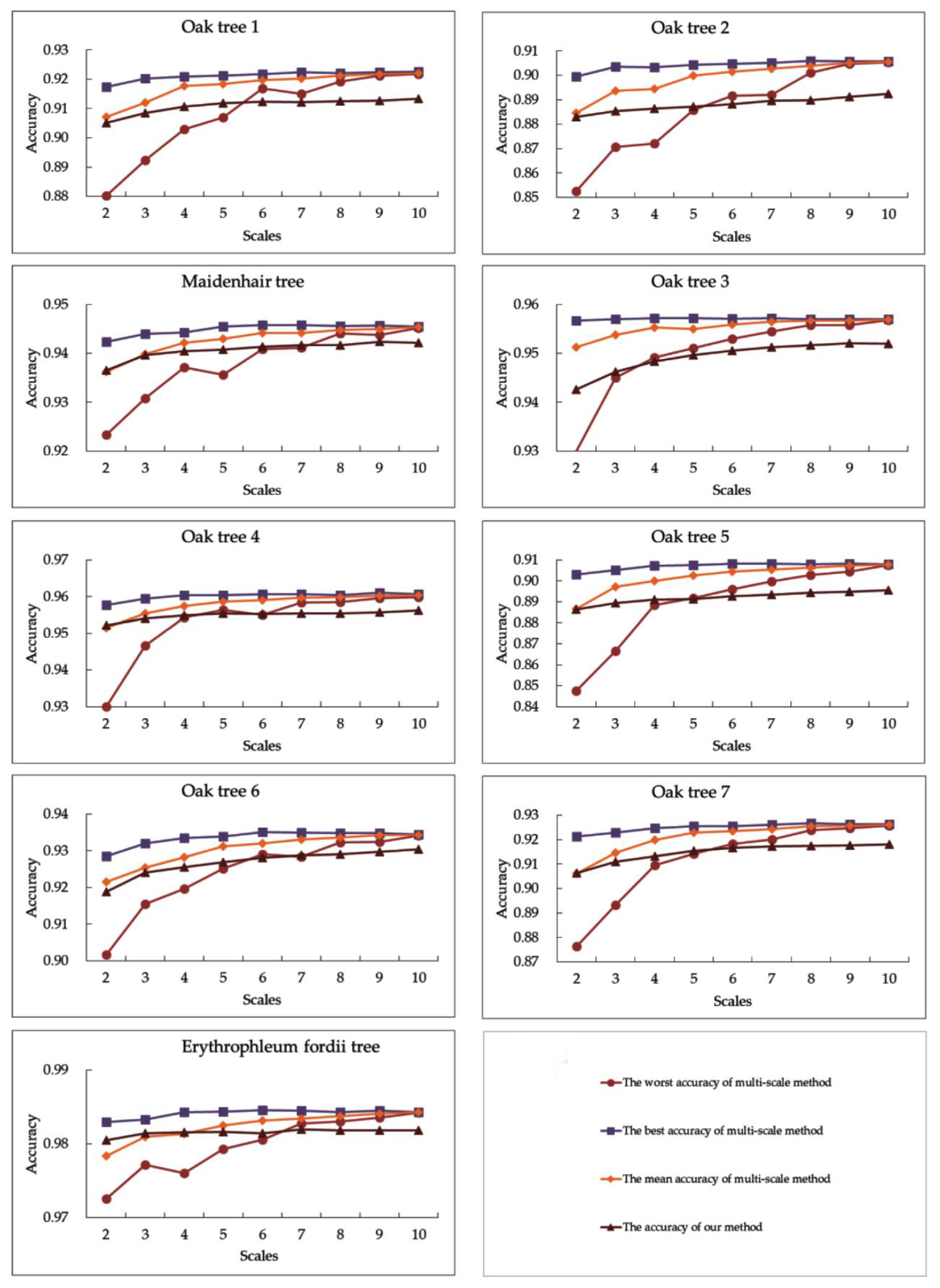
| Trees | Optimal Scale Method | Our Method |
|---|---|---|
| Oak tree 1 | 0.8947 | 0.9133 |
| Oak tree 1 | 0.8738 | 0.8923 |
| Maidenhair tree | 0.9194 | 0.9374 |
| Oak tree 3 | 0.9301 | 0.9521 |
| Oak tree 4 | 0.9452 | 0.9561 |
| Oak tree 5 | 0.8772 | 0.8955 |
| Oak tree 6 | 0.9058 | 0.9304 |
| Oak tree 7 | 0.8904 | 0.9181 |
| Erythrophleum fordii tree | 0.9759 | 0.9820 |
| Trees | With Optimization (s) | Without Optimization (s) | Speedup Ratio |
|---|---|---|---|
| Oak tree 1 | 32.72 | 1714.80 | 52.41 |
| Oak tree 1 | 90.37 | 5425.74 | 60.04 |
| Maidenhair tree | 10.04 | 462.92 | 46.11 |
| Oak tree 3 | 74.41 | 4431.73 | 59.56 |
| Oak tree 4 | 40.95 | 2244.31 | 54.81 |
| Oak tree 5 | 74.98 | 4494.36 | 59.94 |
| Oak tree 6 | 42.63 | 2224.73 | 52.18 |
| Oak tree 7 | 49.75 | 2760.86 | 55.50 |
| Erythrophleum fordii tree | 36.49 | 2004.13 | 54.93 |
© 2019 by the authors. Licensee MDPI, Basel, Switzerland. This article is an open access article distributed under the terms and conditions of the Creative Commons Attribution (CC BY) license (http://creativecommons.org/licenses/by/4.0/).
Share and Cite
Zhou, J.; Wei, H.; Zhou, G.; Song, L. Separating Leaf and Wood Points in Terrestrial Laser Scanning Data Using Multiple Optimal Scales. Sensors 2019, 19, 1852. https://doi.org/10.3390/s19081852
Zhou J, Wei H, Zhou G, Song L. Separating Leaf and Wood Points in Terrestrial Laser Scanning Data Using Multiple Optimal Scales. Sensors. 2019; 19(8):1852. https://doi.org/10.3390/s19081852
Chicago/Turabian StyleZhou, Junjie, Hongqiang Wei, Guiyun Zhou, and Lihui Song. 2019. "Separating Leaf and Wood Points in Terrestrial Laser Scanning Data Using Multiple Optimal Scales" Sensors 19, no. 8: 1852. https://doi.org/10.3390/s19081852
APA StyleZhou, J., Wei, H., Zhou, G., & Song, L. (2019). Separating Leaf and Wood Points in Terrestrial Laser Scanning Data Using Multiple Optimal Scales. Sensors, 19(8), 1852. https://doi.org/10.3390/s19081852