Tracking Multiple Targets from Multistatic Doppler Radar with Unknown Probability of Detection


Abstract
:1. Introduction
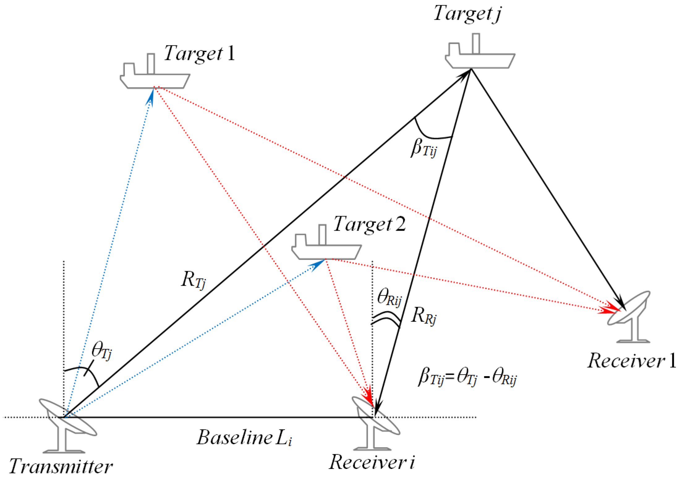
2. Multistatic Doppler Measurement Model
3. Background
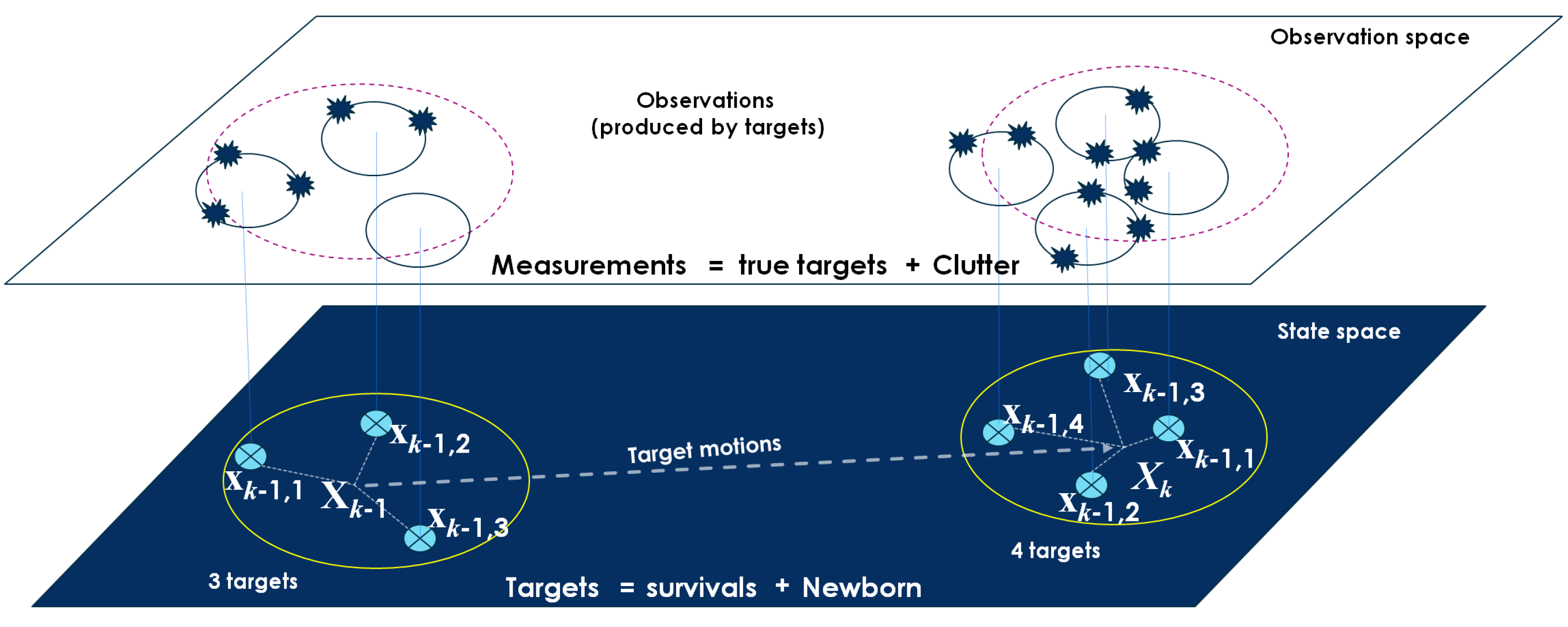
3.1. Labeled RFS
3.2. Bayesian Multitarget Recursion
3.3. Multitarget State Model
3.4. Multitarget Observation Model
3.5. Multisensor GLMB Recursion
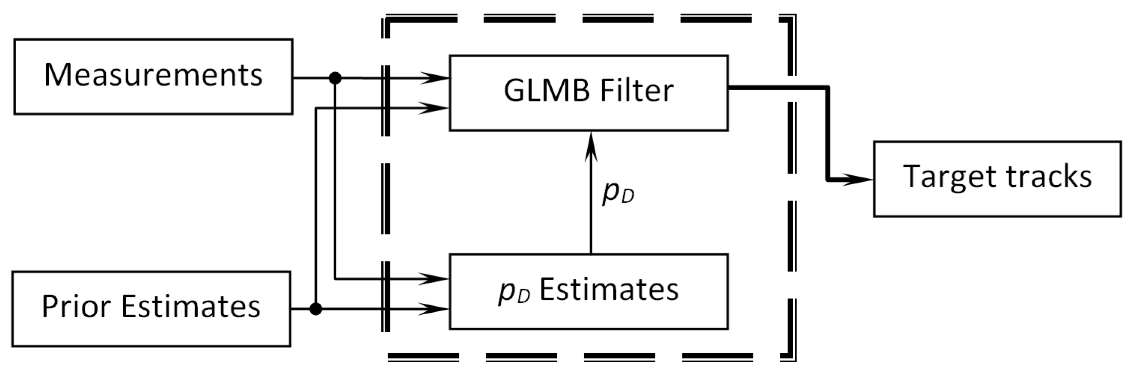
3.6. Adaptive to Unknown Detection Probability
3.7. Implementation
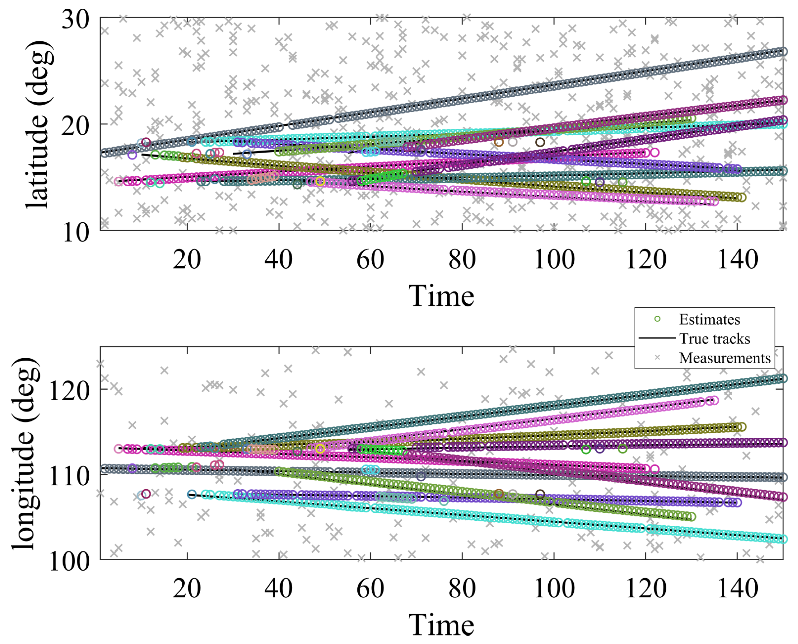
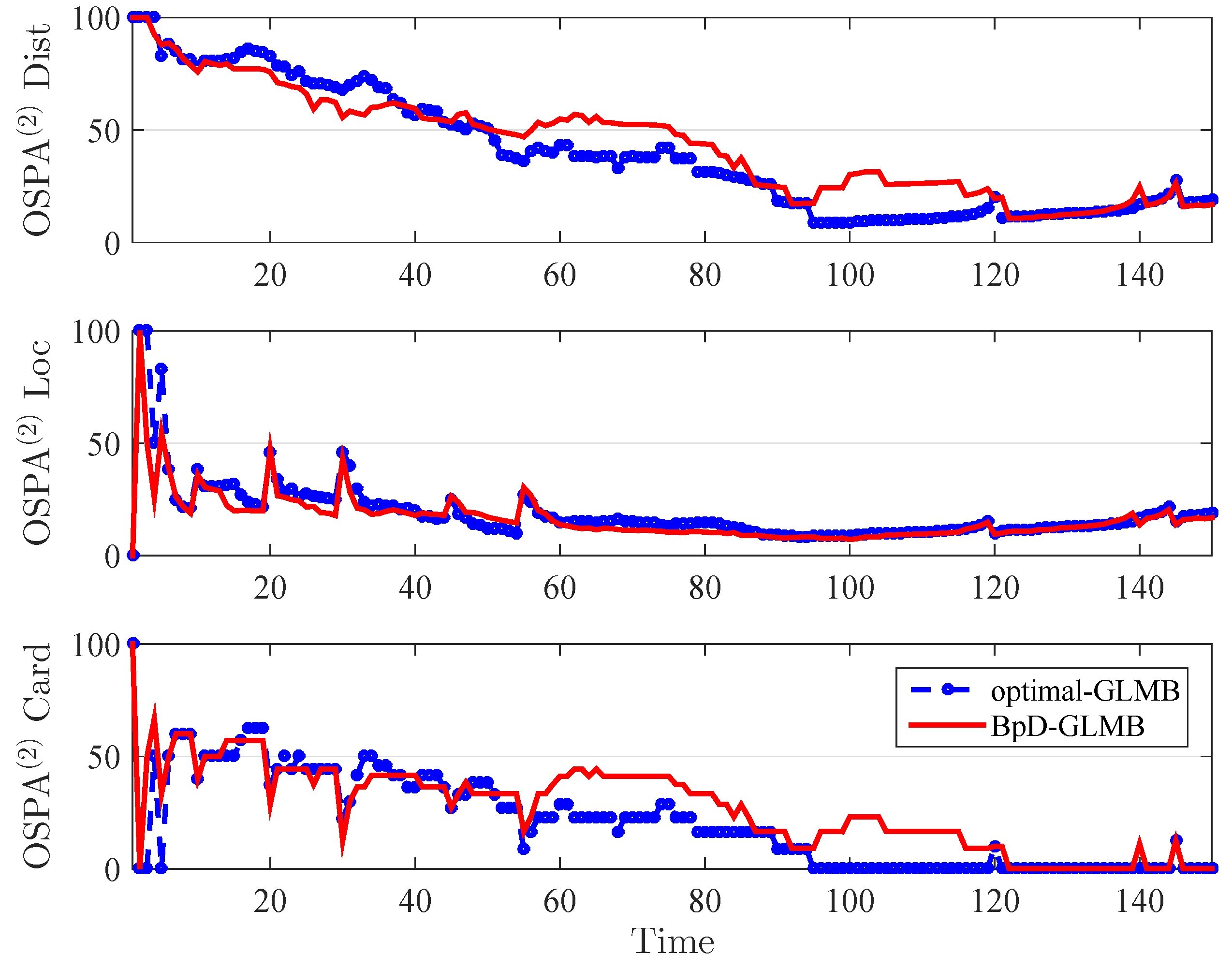
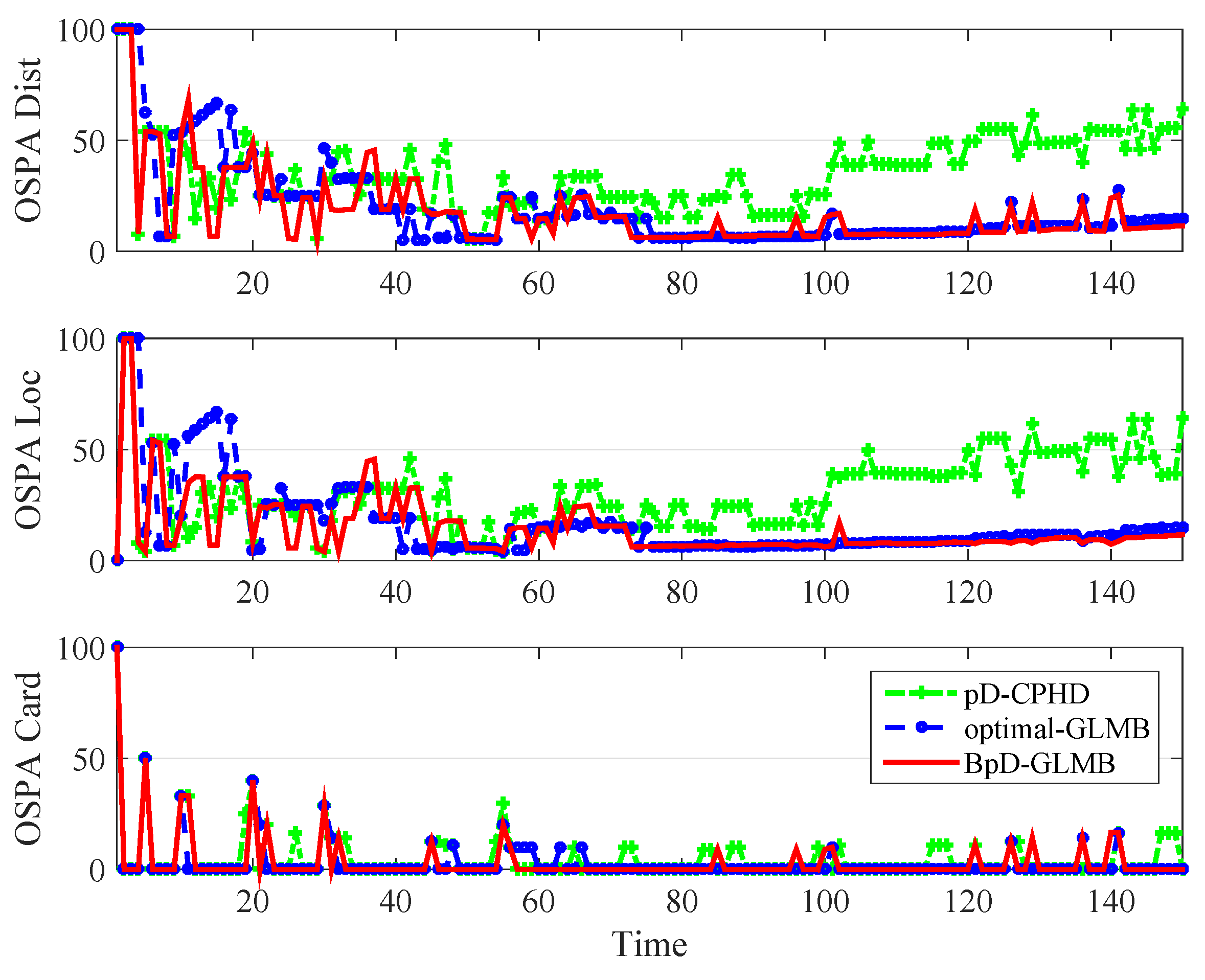
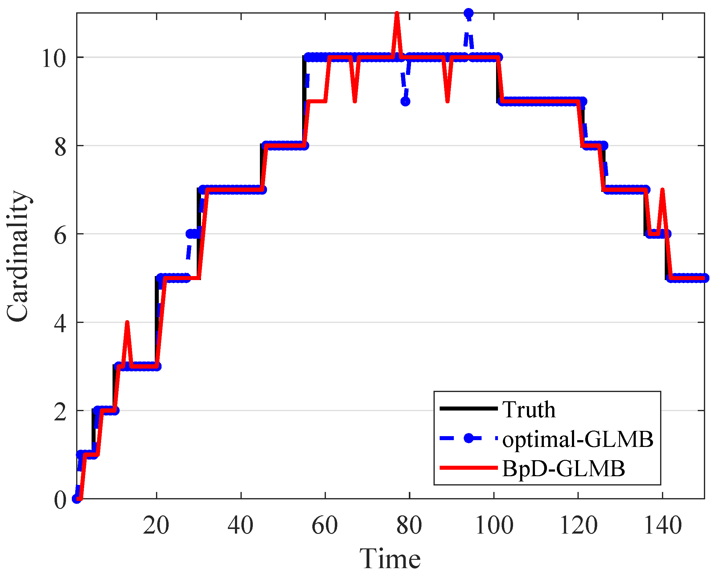
4. Numerical Studies
5. Conclusions
Author Contributions
Funding
Acknowledgments
Conflicts of Interest
References
- Chernyak, V.S. Fundamentals of Multisite Radar Systems: Multistatic Radars and Multistatic Radar Systems; Routledge: Boca Raton, FL, USA, 2018; ISBN 978-90-5699-165-4. [Google Scholar]
- Le Chevalier, F. Principles of Radar and Sonar Signal Processing; Artech House: Boston, MA, USA, 2002; ISBN 978-16-3081-229-4. [Google Scholar]
- IEEE. IEEE standard for radar definitions. IEEE P686/D2, 2017 (Revision of IEEE Std 686-2008); IEEE: New York, NY, USA, 2017; pp. 1–54. [Google Scholar]
- Griffiths, H.D.; Baker, C.J. An Introduction to Passive Radar; Artech House: London, UK, 2017; ISBN 978-16-3081-036-8. [Google Scholar]
- Chernyak, V.S. Multisite Radar Systems With Information Fusion: A Technology of Xxi Century. Available online: https://www.researchgate.net/profile/Victor_Chernyak/publication/255664974_Multisite_Radar_Systems_with_Information_Fusion_A_Technology_of_XXI_Century/links/0f3175368846840370000000/Multisite-Radar-Systems-with-Information-Fusion-A-Technology-of-XXI-Century.pdf (accessed on 4 April 2019).
- Vo, B.-N.; Mallick, M.; Bar-shalom, Y.; Coraluppi, S.; Osborne, R., III; Mahler, R.; Vo, B.-T. Multitarget tracking. Wiley Encycl. Electr. Electron. Eng. 1999, 1–15. [Google Scholar] [CrossRef]
- Goodman, N.A.; Bruyere, D. Optimum and decentralized detection for multistatic airborne radar. IEEE Trans. Aerosp. Electron. Syst. 2007, 43. [Google Scholar] [CrossRef]
- Smith, G.; Woodbridge, K.; Baker, C.; Griffiths, H. Multistatic micro-doppler radar signatures of personnel targets. IET Signal Process. 2010, 4, 224–233. [Google Scholar] [CrossRef]
- Mahler, R.P. “statistic 103” for multitarget tracking. Sensors 2019, 19, 202. [Google Scholar] [CrossRef] [PubMed]
- Mahler, R.P. Statistical Multisource-Multitarget Information Fusion; Artech House: Boston, MA, USA, 2007; ISBN 978-15-9693-092-6. [Google Scholar]
- Mahler, R.P. Advances in Statistical Multisource-Multitarget Information Fusion; Artech House: Boston, MA, USA, 2014; ISBN 978-16-0807-798-4. [Google Scholar]
- Mahler, R.P. Multitarget bayes filtering via first-order multitarget moments. IEEE Trans. Aerosp. Electron. Syst. 2003, 39, 1152–1178. [Google Scholar] [CrossRef]
- Vo, B.-N.; Singh, S.; Doucet, A. Sequential Monte Carlo methods for multitarget filtering with random finite sets. IEEE Trans. Aerosp. Electron. Syst. 2005, 41, 1224–1245. [Google Scholar] [CrossRef]
- Mahler, R.P. Phd filters of higher order in target number. IEEE Trans. Aerosp. Electron. Syst. 2007, 43. [Google Scholar] [CrossRef]
- Vo, B.-T.; Vo, B.-N.; Cantoni, A. Analytic implementations of the cardinalized probability hypothesis density filter. IEEE Trans. Signal Process. 2007, 55, 3553–3567. [Google Scholar] [CrossRef]
- Vo, B.-N.; Vo, B.-T.; Pham, N.-T.; Suter, D. Joint detection and estimation of multiple objects from image observations. IEEE Trans. Signal Process. 2010, 58, 5129–5141. [Google Scholar] [CrossRef]
- Vo, B.-T.; Vo, B.-N.; Cantoni, A. The cardinality balanced multi-target multi-bernoulli filter and its implementations. IEEE Trans. Signal Process. 2009, 57, 409–423. [Google Scholar] [CrossRef]
- Vo, B.-T.; Vo, B.-N. Labeled random finite sets and multi-object conjugate priors. IEEE Trans. Signal Process. 2013, 61, 3460–3475. [Google Scholar] [CrossRef]
- Vo, B.-N.; Vo, B.-T.; Phung, D. Labeled random finite sets and the Bayes multi-target tracking filter. IEEE Trans. Signal Process. 2014, 62, 6554–6567. [Google Scholar] [CrossRef]
- Reuter, S.; Vo, B.-T.; Vo, B.-N.; Dietmayer, K. The labeled multi-Bernoulli filter. IEEE Trans. Signal Process. 2014, 62, 3246–3260. [Google Scholar] [CrossRef]
- Vo, B.-T.; Vo, B.-N. Multi-scan generalized labeled multi-Bernoulli filter. In Proceedings of the IEEE 21st International Conference on Information Fusion (FUSION 2018), Cambridge, UK, 10–13 July 2018; pp. 195–202. [Google Scholar]
- Vo, B.-N.; Vo, B.-T.; Hoang, H.G. An efficient implementation of the generalized labeled multi-bernoulli filter. IEEE Trans. Signal Process. 2017, 65, 1975–1987. [Google Scholar] [CrossRef]
- Beard, M.; Vo, B.-T.; Vo, B.-N. Bayesian multi-target tracking with merged measurements using labelled random finite sets. IEEE Trans. Signal Process. 2015, 63, 1433–1447. [Google Scholar] [CrossRef]
- Beard, M.; Reuter, S.; Granström, K.; Vo, B.-T.; Vo, B.-N.; Scheel, A. Multiple extended target tracking with labeled random finite sets. IEEE Trans. Signal Process. 2016, 64, 1638–1653. [Google Scholar] [CrossRef]
- Yi, W.; Jiang, M.; Hoseinnezhad, R. The multiple model Vo–Vo filter. IEEE Trans. Aerosp. Electron. Syst. 2017, 53, 1045–1054. [Google Scholar] [CrossRef]
- Papi, F.; Kim, D.Y. A particle multi-target tracker for superpositional measurements using labeled random finite sets. IEEE Trans. Signal Process. 2015, 63, 4348–4358. [Google Scholar] [CrossRef]
- Li, S.; Yi, W.; Hoseinnezhad, R.; Wang, B.; Kong, L. Multiobject tracking for generic observation model using labeled random finite sets. IEEE Trans. Signal Process. 2018, 66, 368–383. [Google Scholar] [CrossRef]
- Punchihewa, Y.G.; Vo, B.-T.; Vo, B.-N.; Kim, D.Y. Multiple object tracking in unknown backgrounds with labeled random finite sets. IEEE Trans. Signal Process. 2018, 66, 3040–3055. [Google Scholar] [CrossRef]
- Kim, D.Y.; Vo, B.-N.; Vo, B.-T. Online visual multi-object tracking via labeled random finite set filtering. arXiv, 2016; arXiv:1611.06011. [Google Scholar]
- Beard, M.; Vo, B.-T.; Vo, B.-N.; Arulampalam, S. Void probabilities and Cauchy–Schwarz divergence for generalized labeled multi-Bernoulli models. IEEE Trans. Signal Process. 2017, 65, 5047–5061. [Google Scholar] [CrossRef]
- Wang, X.; Hoseinnezhad, R.; Gostar, A.K.; Rathnayake, T.; Xu, B.; Bab-Hadiashar, A. Multi-sensor control for multi-object bayes filters. Signal Process. 2018, 142, 260–270. [Google Scholar] [CrossRef]
- Fantacci, C.; Vo, B.N.; Vo, B.-T.; Battistelli, G.; Chisci, L. Robust fusion for multisensor multiobject tracking. IEEE Signal Process. Lett. 2018, 25, 640–644. [Google Scholar] [CrossRef]
- Deusch, H.; Reuter, S.; Dietmayer, K. The labeled multi-Bernoulli slam filter. IEEE Signal Process. Lett. 2015, 22, 1561–1565. [Google Scholar] [CrossRef]
- Hadden, W.J.; Young, J.L.; Holle, A.W.; McFetridge, M.L.; Kim, D.Y.; Wijesinghe, P.; Taylor-Weiner, H.; Wen, J.H.; Lee, A.R.; Bieback, K.; et al. Stem cell migration and mechanotransduction on linear stiffness gradient hydrogels. In Proceedings of the National Academy of Sciences (PNAS 2017), 30 May 2017; pp. 5551–5553. [Google Scholar] [CrossRef]
- Vo, B.-N.; Dam, N.; Phung, D.; Tran, Q.; Vo, B.-T. Model-based learning for point pattern data. Pattern Recogn. 2018, 84, 136–151. [Google Scholar] [CrossRef]
- Beard, M.; Vo, B.-T.; Vo, B.-N. A solution for large-scale multi-object tracking. arXiv, 2018; arXiv:1804.06622. [Google Scholar]
- Tobias, M.; Lanterman, A.D. A probability hypothesis density-based multitarget tracker using multiple bistatic range and velocity measurements. In Proceedings of the Thirty-Sixth Southeastern Symposium on System Theory (SSST 04), Atlanta, GA, USA, 16 March 2004; pp. 205–209. [Google Scholar]
- Liang, M.; Kim, D.Y.; Kai, X. Multi-bernoulli filter for target tracking with multi-static doppler only measurement. Signal Process. 2015, 108, 102–110. [Google Scholar] [CrossRef]
- Do, C.-T.; Nguyen, H.V. Multistatic Doppler-based marine ships tracking. In Proceedings of the International Conference on Control, Automation and Information Sciences (ICCAIS 2018), IEEE, Hangzhou, China, 24–27 October 2018; pp. 151–156. [Google Scholar]
- Battistelli, G.; Chisci, L.; Morrocchi, S.; Papi, F.; Farina, A.; Graziano, A. Robust multisensor multitarget tracker with application to passive multistatic radar tracking. IEEE Trans. Aerosp. Electron. Syst. 2012, 48, 3450–3472. [Google Scholar] [CrossRef]
- Chernyak, V.S. Using mimo radars in multisite radar systems. In Proceedings of the International Radar Symposium (IRS), Leipzig, Germany, 7–9 November 2011; pp. 691–696. [Google Scholar]
- Chernyak, V.S. Multisite radar systems composed of mimo radars. IEEE Aerosp. Electron. Syst. Mag. 2014, 29, 28–37. [Google Scholar] [CrossRef]
- Chetty, K.; Woodbridge, K.; Guo, H.; Smith, G.E. Passive bistatic wimax radar for marine surveillance. In Proceedings of the 2010 IEEE Radar Conference, Arlington, VA, USA, 10–14 May 2010; pp. 188–193. [Google Scholar]
- Guldogan, M.B.; Lindgren, D.; Gustafsson, F.; Habberstad, H.; Orguner, U. Multi-target tracking with phd filter using doppler-only measurements. Digital Signal Process. 2014, 27, 1–11. [Google Scholar] [CrossRef]
- Mahler, R.P.; Vo, B.-T.; Vo, B.-N. Cphd filtering with unknown clutter rate and detection profile. IEEE Trans. Signal Process. 2011, 59, 3497–3513. [Google Scholar] [CrossRef]
- Li, S.; Yi, W.; Hoseinnezhad, R.; Battistelli, G.; Wang, B.; Kong, L. Robust distributed fusion with labeled random finite sets. IEEE Trans. Signal Process. 2018, 66, 278–293. [Google Scholar] [CrossRef]
- Vo, B.-T.; Vo, B.-N.; Hoseinnezhad, R.; Mahler, R.P. Robust multi-Bernoulli filtering. IEEE J. Sel. Top. Signal Process. 2013, 7, 399–409. [Google Scholar] [CrossRef]
- Doviak, R.J.; Zrnic, D.S. Doppler Radar and Weather Observations, 2nd ed.; Dover Publications: Saint Louis, NY, USA, 2006; ISBN 978-04-8645-060-5. [Google Scholar]
- Guo, F.; Fan, Y.; Zhou, Y.; Xhou, C.; Li, Q. Space Electronic Reconnaissance: Localization Theories and Methods, 1st ed.; John Wiley & Sons: Hoboken, NJ, USA, 2014; ISBN 978-11-1854-219-4. [Google Scholar]
- Vo, B.-T.; Vo, B.-N.; Cantoni, A. Bayesian filtering with random finite set observations. IEEE Trans. Signal Process. 2008, 56, 1313–1326. [Google Scholar] [CrossRef]
- Mallick, M.; Krishnamurthy, V.; Vo, B.-N. Integrated Tracking, Classification, and Sensor Management; IEEE Press: Piscataway, NJ, USA, 2013; p. 77. ISBN 978-0-470-63905-4. [Google Scholar]
- Vo, B.-N.; Vo, B.-T. An implementation of the multi-sensor generalized labeled multi-Bernoulli filter via Gibbs sampling. In Proceedings of the 20th International Conference on Information Fusion (Fusion 2017), IEEE, Xi’an, China, 10–13 July 2017; pp. 1–8. [Google Scholar]
- Mahler, R.P.; El-Fallah, A. Cphd filtering with unknown probability of detection. Proc. SPIE 2010. [Google Scholar] [CrossRef]
- Mahler, R.P.; El-Fallah, A. Cphd and phd filters for unknown backgrounds, part iii: Tractable multitarget filtering in dynamic clutter. Proc. SPIE 2010. [Google Scholar] [CrossRef]
- Julier, S.J.; Uhlmann, J.K. Unscented filtering and nonlinear estimation. Proc. IEEE 2004, 92, 401–422. [Google Scholar] [CrossRef]
- Wei, B.; Nener, B.; Liu, W.; Ma, L. Centralized multi-sensor multi-target tracking with labeled random finite sets. In Proceedings of the 2016 International Conference on Control, Automation and Information Sciences (ICCAIS 2016), Ansan, Korea, 27–29 October 2016; pp. 82–87. [Google Scholar]
- Schuhmacher, D.; Vo, B.-T.; Vo, B.-N. A consistent metric for performance evaluation of multi-object filters. IEEE Trans. Signal Process. 2008, 56, 3447–3457. [Google Scholar] [CrossRef]


| Parameter | Symbol | Value |
|---|---|---|
| Sample period | 0.15 (h) | |
| Std. of the velocity noise | 0.3 | |
| Std. of the course noise | 180 (rad ) | |
| Common existence probabilities | ||
| Survival probability | 0.98 | |
| Number of targets | N | 10 |
| Target | Init. Position | Init. Speed (kn) | Init. Course (rad/s) | Time of Birth (h) | Time of Death (h) |
|---|---|---|---|---|---|
| T1 | [32, −5] | 1 | 150 | ||
| T2 | [13, −9] | 5 | 120 | ||
| T3 | [−18, 5] | 10 | 140 | ||
| T4 | [2, 32] | 20 | 150 | ||
| T5 | [6, −20] | 20 | 150 | ||
| T6 | [−12, −4] | 30 | 140 | ||
| T7 | [15, −30] | 30 | 130 | ||
| T8 | [−15, 30] | 45 | 135 | ||
| T9 | [28, −30] | 55 | 150 | ||
| T10 | [30, 5] | 55 | 150 |
| Name | Symbol | Value |
|---|---|---|
| Transmitter | ||
| Receiver 1 | ||
| Receiver 2 | ||
| Transmit frequency | 900 MHz | |
| Speed of light | c | |
| Initial detection probabilities | [] | [0.70; 0.98] |
| Average clutter rate | [] | [10; 25] |
© 2019 by the authors. Licensee MDPI, Basel, Switzerland. This article is an open access article distributed under the terms and conditions of the Creative Commons Attribution (CC BY) license (http://creativecommons.org/licenses/by/4.0/).
Share and Cite
Do, C.-T.; Van Nguyen, H. Tracking Multiple Targets from Multistatic Doppler Radar with Unknown Probability of Detection. Sensors 2019, 19, 1672. https://doi.org/10.3390/s19071672
Do C-T, Van Nguyen H. Tracking Multiple Targets from Multistatic Doppler Radar with Unknown Probability of Detection. Sensors. 2019; 19(7):1672. https://doi.org/10.3390/s19071672
Chicago/Turabian StyleDo, Cong-Thanh, and Hoa Van Nguyen. 2019. "Tracking Multiple Targets from Multistatic Doppler Radar with Unknown Probability of Detection" Sensors 19, no. 7: 1672. https://doi.org/10.3390/s19071672
APA StyleDo, C.-T., & Van Nguyen, H. (2019). Tracking Multiple Targets from Multistatic Doppler Radar with Unknown Probability of Detection. Sensors, 19(7), 1672. https://doi.org/10.3390/s19071672