Orientation-Constrained System for Lamp Detection in Buildings Based on Computer Vision

 , ,
, ,  , and
, and 
Abstract
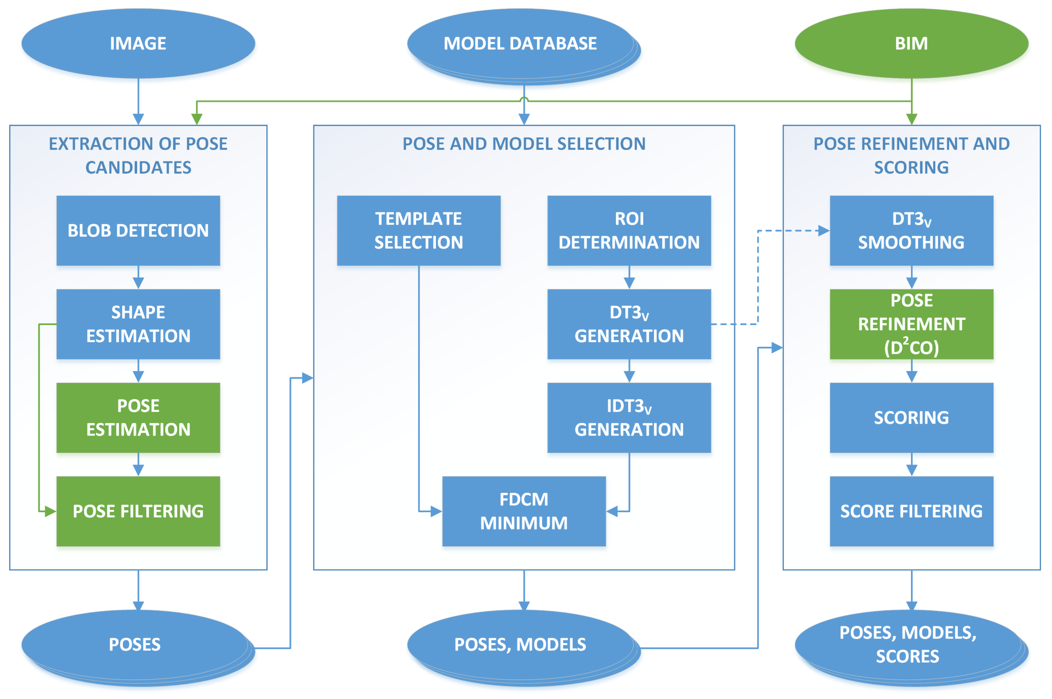
1. Introduction
2. Materials and Methods
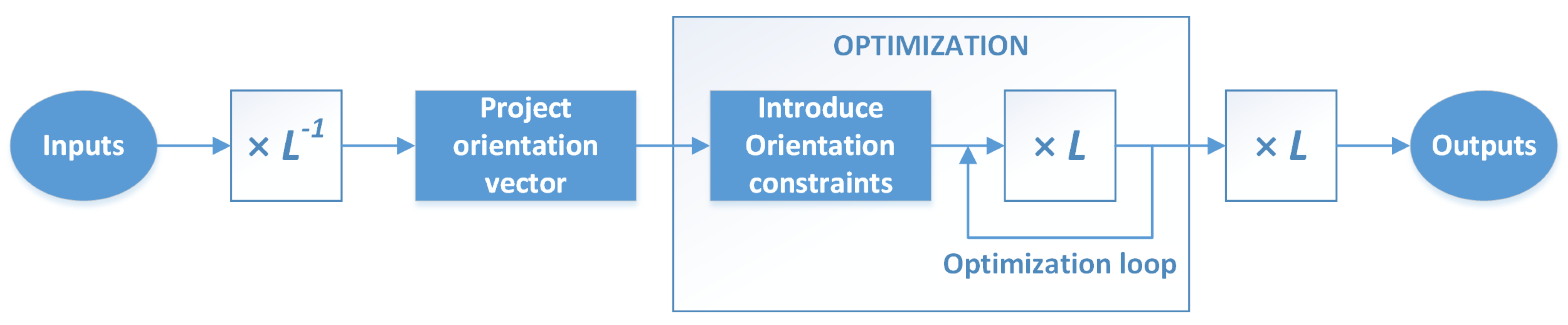
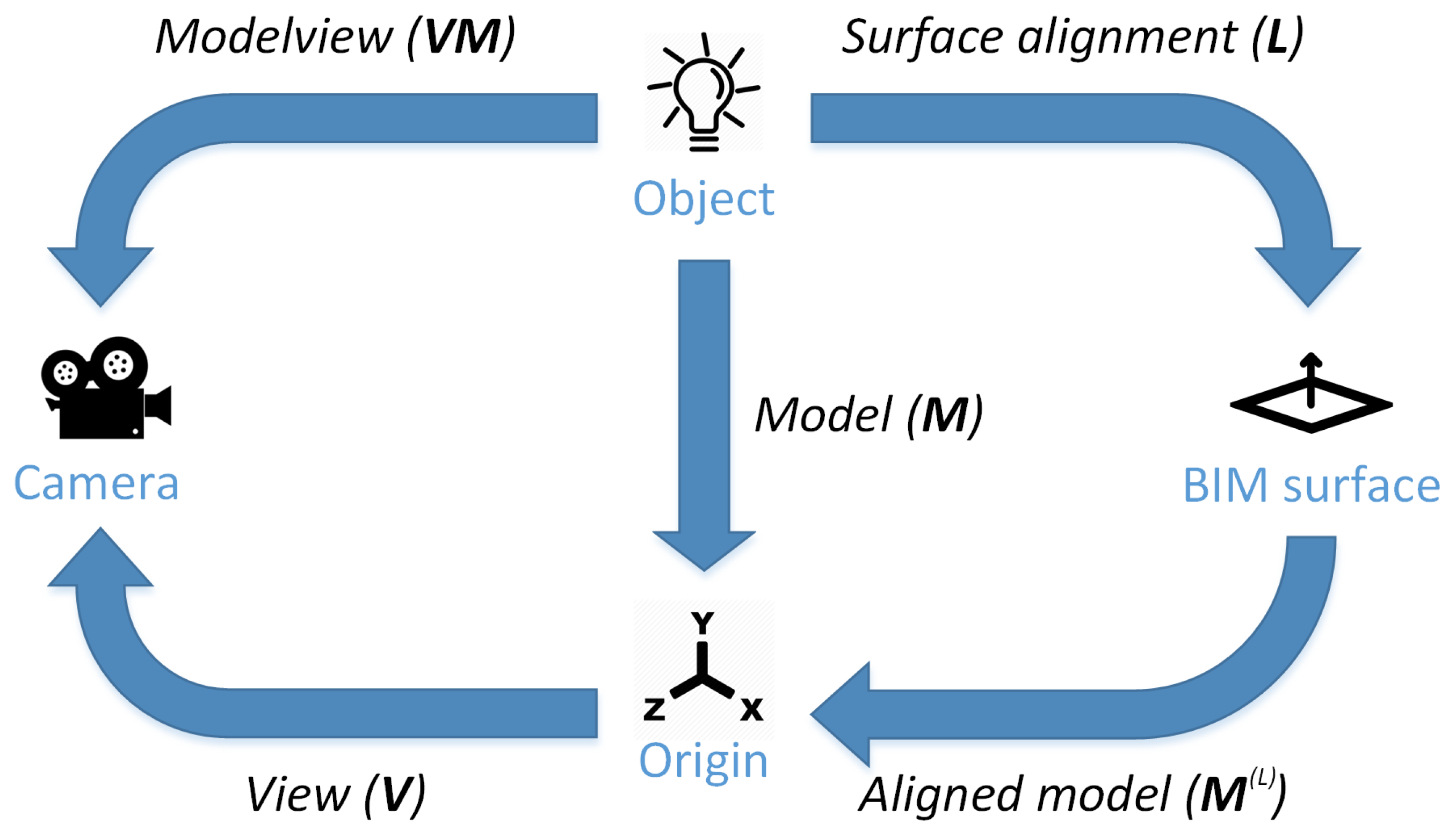
2.1. Orientation Alignment in Optimization Problems
- Calculate an aligned model matrix , with a corresponding orientation vector .
- Project the vector to the z axis, setting the first two components to zero. The result is , as presented in Equation (4), with the corresponding transformation matrix , being a unit normal vector along the z axis:
- Use in the optimization problem, constraining it to changes only in the third component of this vector and performing the projections as presented in (5):Thus, the degrees of freedom for the problem were reduced from six to four.
- Calculate the final optimized model pose from the result of the optimization process, : .
2.2. Pose Estimation
2.2.1. Polygonal Shapes
2.2.2. Circular Shapes
2.3. Pose Refinement
2.4. Pose Filtering
- First, the projected camera point on the plane was obtained, again, using the equations of the projection line and the circle plane . This equation system is presented in Equation (13), with the camera center and :
- The intersection between the line and the circumference with radius was obtained by solving the system of equations in (14), comprising the line from the circle center to , and the circumference of the object:
- Choosing the result in the same quadrant gives the closest intersection that is used as the corresponding object point for .
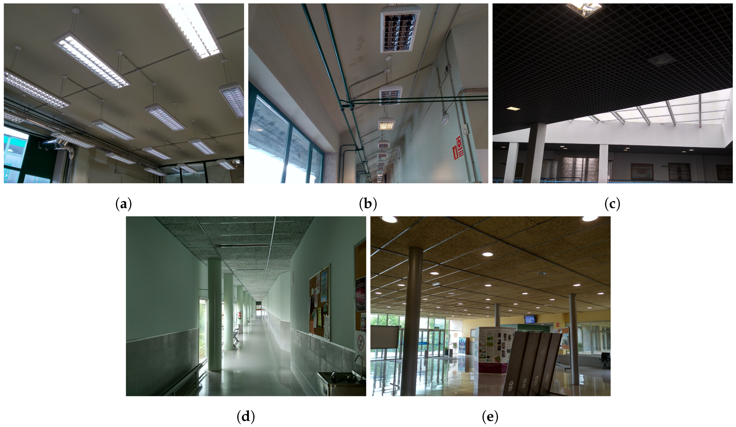
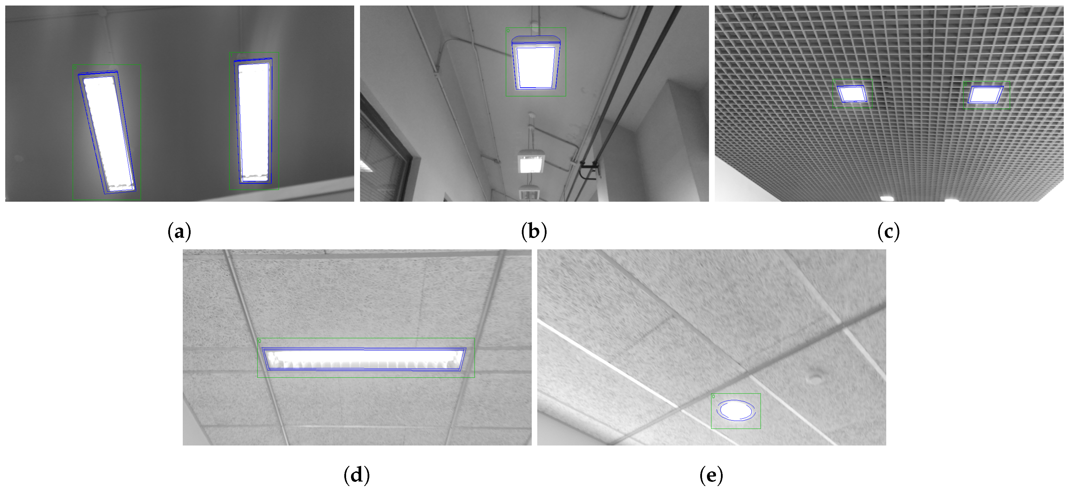
3. Experimental System
4. Results and Discussion
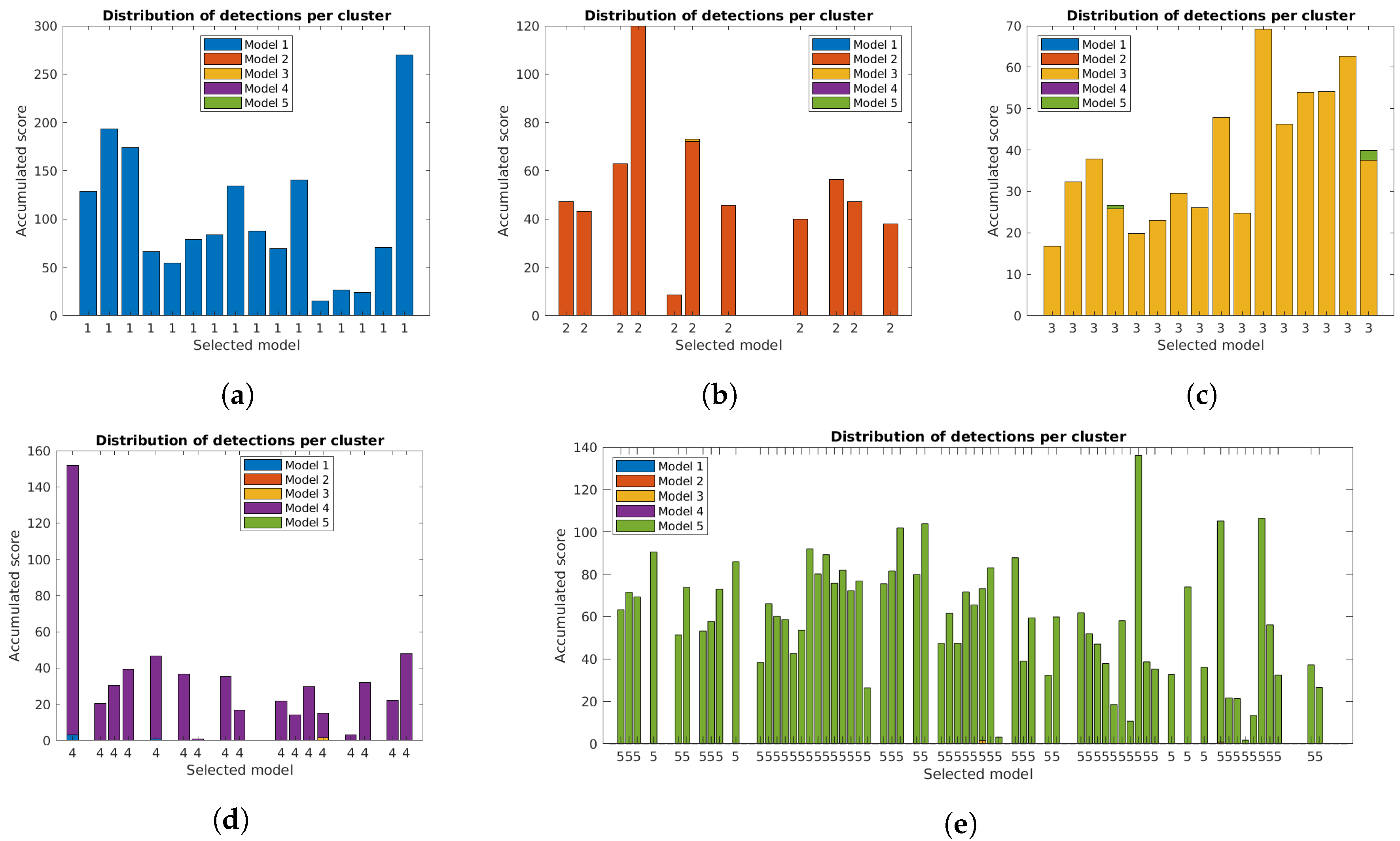
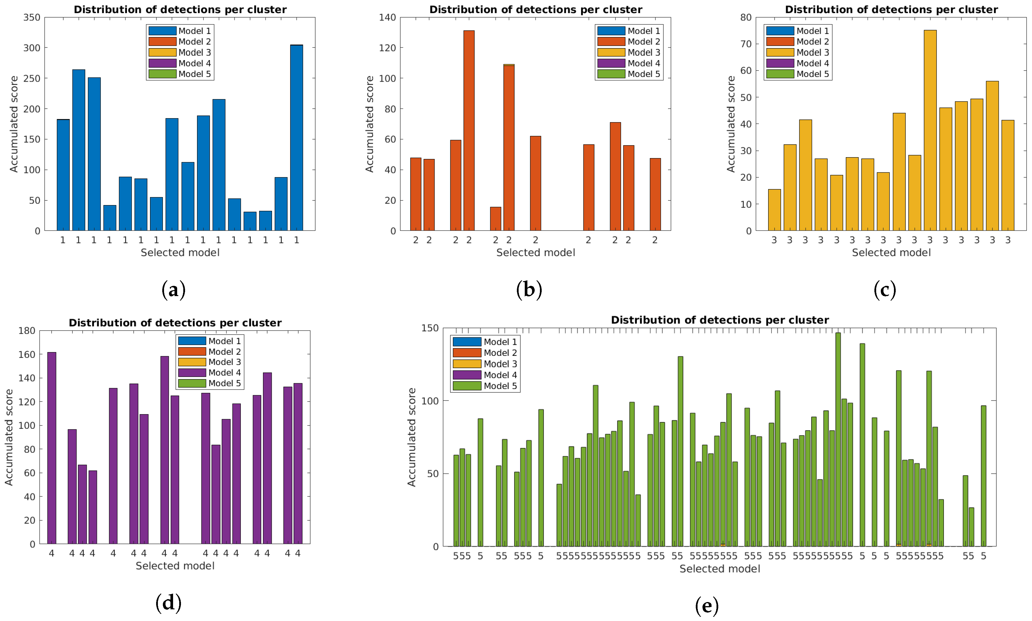
4.1. Number of Detections
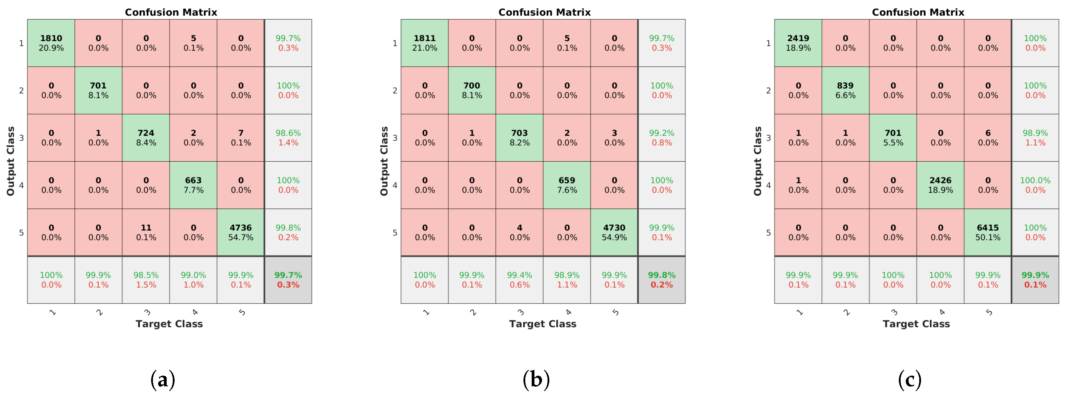
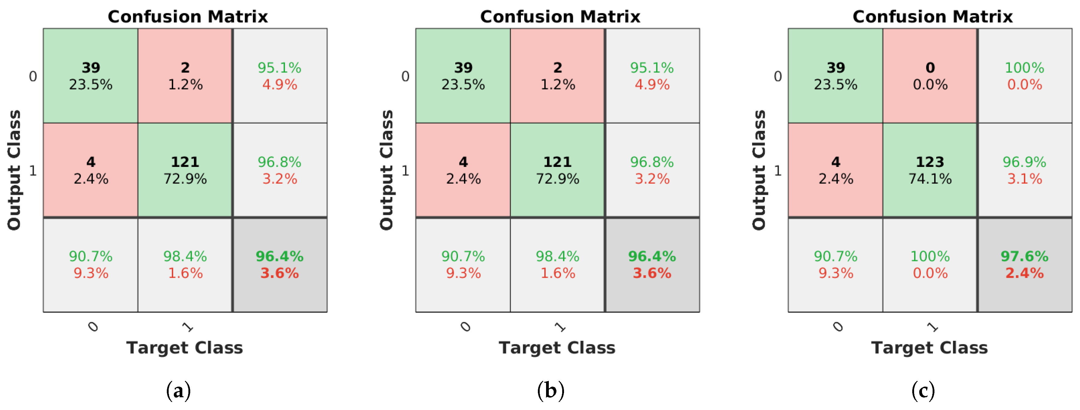
4.2. Identification Rate
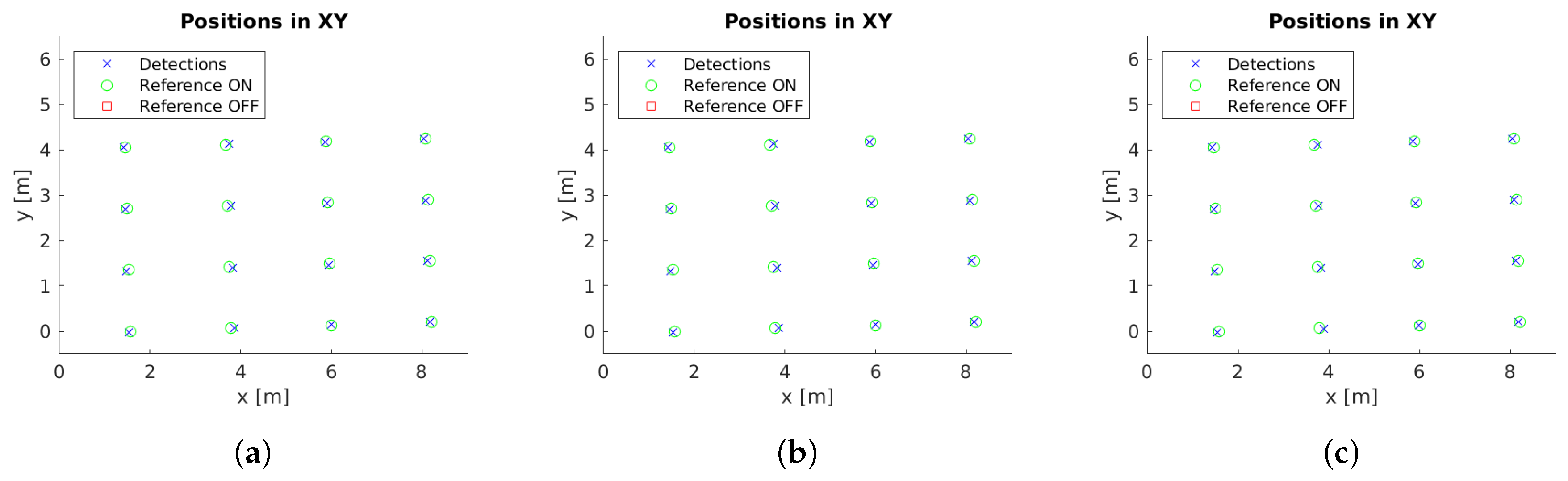
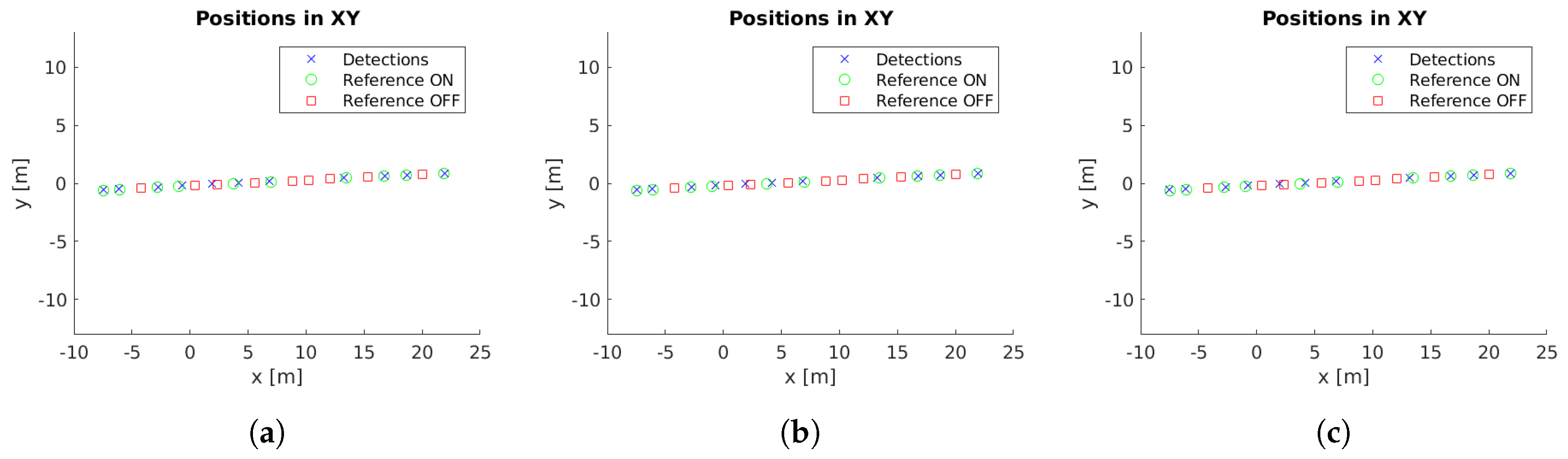
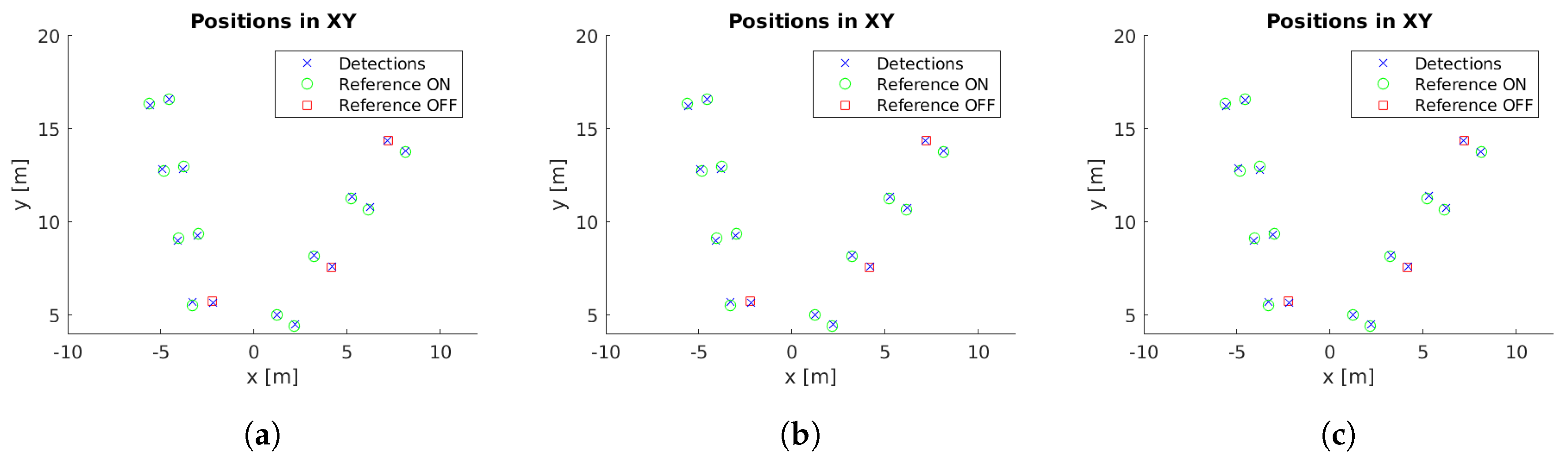
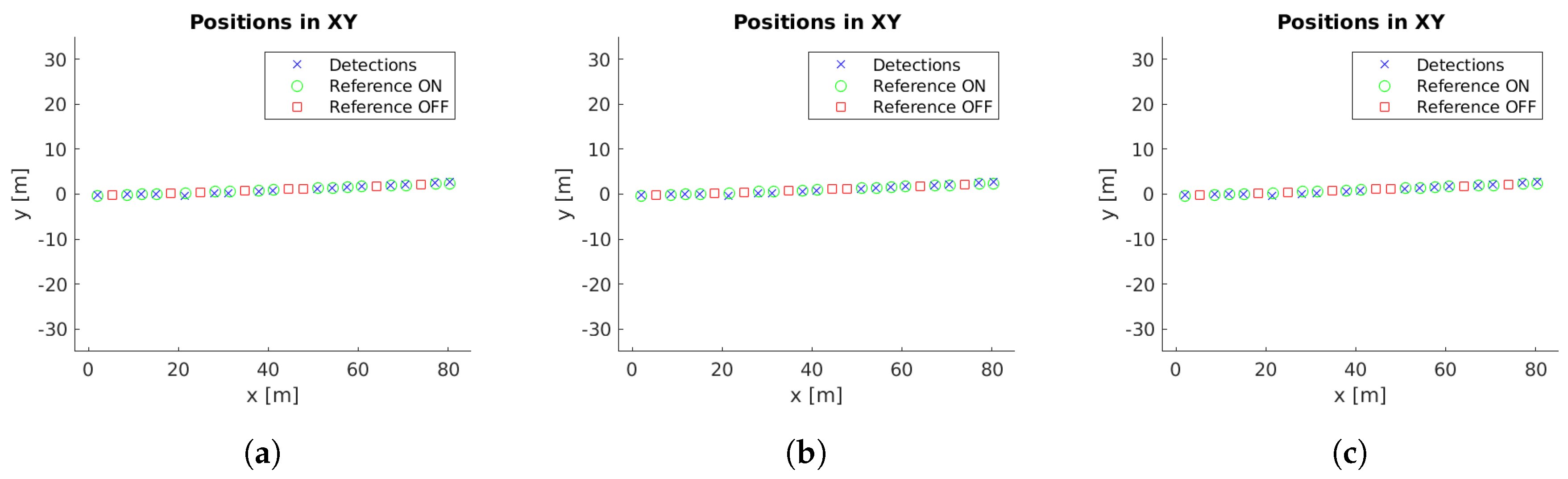
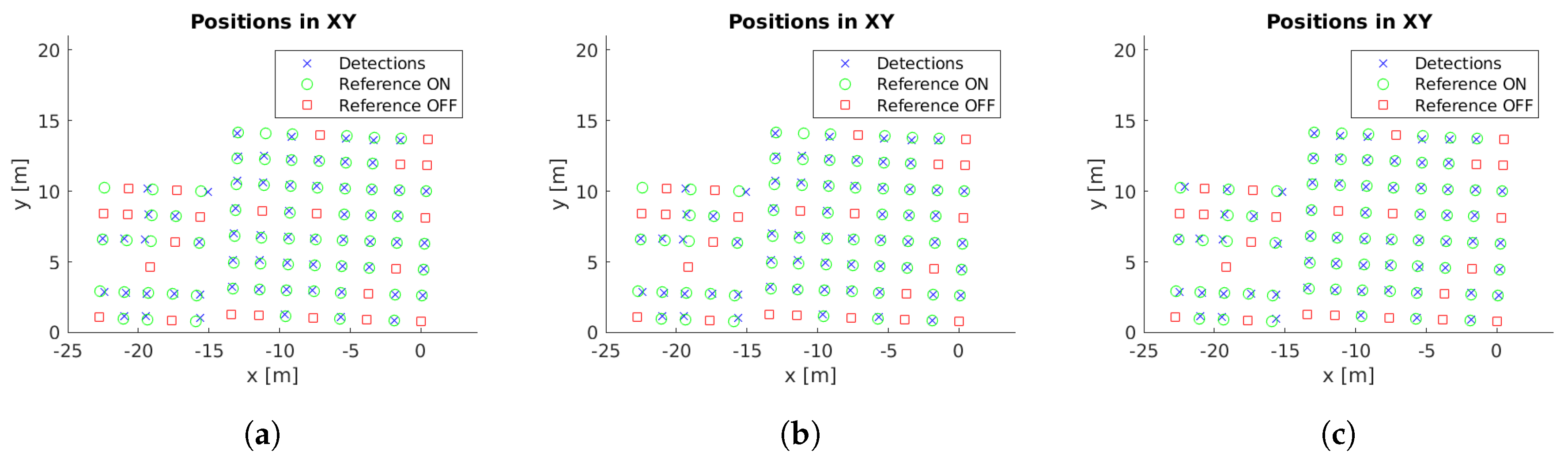
4.3. Distance to Reference
4.4. Applications and Future Work
5. Conclusions
Author Contributions
Funding
Conflicts of Interest
Abbreviations
| BIM | Building information modelling |
| IFC | Industry foundation classes |
| gbXML | Green Building XML Schema |
| LED | Light emitting diode |
| CVS | Computer vision system |
| SIFT | Scale-invariant feature transform |
| SURF | Speeded-up robust features |
| BOLD | Bunch of lines descriptor |
| BORDER | Bounding oriented-rectangle descriptors for enclosed regions |
| BIND | Binary integrated net descriptors |
| FDCM | Fast directional chamfer matching |
| D2CO | Direct directional chamfer optimization |
| ROI | Region of interest |
| PnP | Perspective-n-point |
References
- Soori, P.K.; Vishwas, M. Lighting control strategy for energy efficient office lighting system design. Energy Build. 2013, 66, 329–337. [Google Scholar] [CrossRef]
- Pérez-Lombard, L.; Ortiz, J.; Pout, C. A review on buildings energy consumption information. Energy Build. 2008, 40, 394–398. [Google Scholar] [CrossRef]
- Baloch, A.; Shaikh, P.; Shaikh, F.; Leghari, Z.; Mirjat, N.; Uqaili, M. Simulation tools application for artificial lighting in buildings. Renew. Sustain. Energy Rev. 2018, 82, 3007–3026. [Google Scholar] [CrossRef]
- Waide, P.; Tanishima, S. Light’s Labour’s Lost: Policies for Energy-Efficient Lighting: In Support of the G8 Plan of Action; OECD/IEA: Paris, France, 2006. [Google Scholar]
- Sanhudo, L.; Ramos, N.; Poças Martins, J.; Almeida, R.; Barreira, E.; Simões, M.; Cardoso, V. Building information modeling for energy retrofitting—A review. Renew. Sustain. Energy Rev. 2018, 89, 249–260. [Google Scholar] [CrossRef]
- Asl, M.R.; Zarrinmehr, S.; Bergin, M.; Yan, W. BPOpt: A framework for BIM-based performance optimization. Energy Build. 2015, 108, 401–412. [Google Scholar] [CrossRef]
- Succar, B. Building information modelling framework: A research and delivery foundation for industry stakeholders. Autom. Constr. 2009, 18, 357–375. [Google Scholar] [CrossRef]
- IFC4 Add2 Specification. Available online: http://www.buildingsmart-tech.org/specifications/ifc-releases/ifc4-add2 (accessed on 27 March 2019).
- gbXML—An Industry Supported Standard for Storing and Sharing Building Properties between 3D Architectural and Engineering Analysis Software. Available online: http://www.gbxml.org/ (accessed on 27 March 2019).
- Lu, Y.; Wu, Z.; Chang, R.; Li, Y. Building Information Modeling (BIM) for green buildings: A critical review and future directions. Autom. Constr. 2017, 83, 134–148. [Google Scholar] [CrossRef]
- Welle, B.; Rogers, Z.; Fischer, M. BIM-Centric Daylight Profiler for Simulation (BDP4SIM): A methodology for automated product model decomposition and recomposition for climate-based daylighting simulation. Build. Environ. 2012, 58, 114–134. [Google Scholar] [CrossRef]
- Elvidge, C.D.; Keith, D.M.; Tuttle, B.T.; Baugh, K.E. Spectral Identification of Lighting Type and Character. Sensors 2010, 10, 3961–3988. [Google Scholar] [CrossRef]
- Liu, H.; Zhou, Q.; Yang, J.; Jiang, T.; Liu, Z.; Li, J. Intelligent Luminance Control of Lighting Systems Based on Imaging Sensor Feedback. Sensors 2017, 17, 321. [Google Scholar] [CrossRef]
- Imperoli, M.; Pretto, A. D2CO: Fast and robust registration of 3d textureless objects using the directional chamfer distance. Lect. Notes Comput. Sci. 2015, 9163, 316–328. [Google Scholar]
- Lowe, D.G. Distinctive Image Features from Scale-Invariant Keypoints. Int. J. Comput. Vis. 2004, 60, 91–110. [Google Scholar] [CrossRef]
- Bay, H.; Ess, A.; Tuytelaars, T.; Gool, L.V. Speeded-Up Robust Features (SURF). Comput. Vis. Image Underst. 2008, 110, 346–359. [Google Scholar] [CrossRef]
- Tombari, F.; Franchi, A.; Di, L. BOLD Features to Detect Texture-less Objects. In Proceedings of the 2013 IEEE International Conference on Computer Vision, Sydney, Australia, 1–8 December 2013; pp. 1265–1272. [Google Scholar] [CrossRef]
- Chan, J.; Lee, J.A.; Kemao, Q. BORDER: An Oriented Rectangles Approach to Texture-Less Object Recognition. In Proceedings of the 2016 IEEE Conference on Computer Vision and Pattern Recognition (CVPR), Las Vegas, NV, USA, 27–30 June 2016; pp. 2855–2863. [Google Scholar]
- Chan, J.; Lee, J.A.; Kemao, Q. BIND: Binary Integrated Net Descriptors for Texture-Less Object Recognition. In Proceedings of the 2017 IEEE Conference on Computer Vision and Pattern Recognition (CVPR), Honolulu, HI, USA, 21–26 July 2017; pp. 3020–3028. [Google Scholar] [CrossRef]
- Damen, D.; Bunnun, P.; Calway, A.; Mayol-Cuevas, W. Real-time learning and detection of 3D texture-less objects: A scalable approach. In Proceedings of the British Machine Vision Conference, Surrey, UK, 3–7 September 2012. [Google Scholar]
- Hodaň, T.; Damen, D.; Mayol-Cuevas, W.; Matas, J. Efficient texture-less object detection for augmented reality guidance. In Proceedings of the 2015 IEEE International Symposium on Mixed and Augmented Reality Workshops, Fukuoka, Japan, 29 September–3 October 2015; pp. 81–86. [Google Scholar]
- Ferrari, V.; Fevrier, L.; Schmid, C.; Jurie, F. Groups of adjacent contour segments for object detection. IEEE Trans. Pattern Anal. Mach. Intell. 2007, 30, 36–51. [Google Scholar] [CrossRef] [PubMed]
- Ferrari, V.; Jurie, F.; Schmid, C. From Images to Shape Models for Object Detection. Int. J. Comput. Vis. 2010, 87, 284–303. [Google Scholar] [CrossRef]
- Carmichael, O.; Hebert, M. Shape-based recognition of wiry objects. IEEE Trans. Pattern Anal. Mach. Intell. 2004, 26, 1537–1552. [Google Scholar] [CrossRef] [PubMed]
- Barrow, H.G.; Tenenbaum, J.M.; Bolles, R.C.; Wolf, H.C. Parametric Correspondence and Chamfer Matching: Two New Techniques for Image Matching. In Proceedings of the 5th International Joint Conference on Artificial Intelligence, Cambridge, MA, USA, 22–25 August 1977; Morgan Kaufmann Publishers Inc.: San Francisco, CA, USA, 1977; Volume 2, pp. 659–663. [Google Scholar]
- Borgefors, G. Hierarchical chamfer matching: A parametric edge matching algorithm. IEEE Trans. Pattern Anal. Mach. Intell. 1988, 10, 849–865. [Google Scholar] [CrossRef]
- Shotton, J.; Blake, A.; Cipolla, R. Multiscale Categorical Object Recognition Using Contour Fragments. IEEE Trans. Pattern Anal. Mach. Intell. 2008, 30, 1270–1281. [Google Scholar] [CrossRef]
- Hinterstoisser, S.; Cagniart, C.; Ilic, S.; Sturm, P.; Navab, N.; Fua, P.; Lepetit, V. Gradient Response Maps for Real-Time Detection of Textureless Objects. IEEE Trans. Pattern Anal. Mach. Intell. 2012, 34, 876–888. [Google Scholar] [CrossRef]
- Liu, M.Y.; Tuzel, O.; Veeraraghavan, A.; Chellappa, R. Fast Directional Chamfer Matching. In Proceedings of the 2010 IEEE Computer Society Conference on Computer Vision and Pattern Recognition, San Francisco, CA, USA, 13–18 June 2010. [Google Scholar]
- Troncoso-Pastoriza, F.; Eguía-Oller, P.; Díaz-Redondo, R.P.; Granada-Álvarez, E. Generation of BIM data based on the automatic detection, identification and localization of lamps in buildings. Sustain. Cities Soc. 2018, 36, 59–70. [Google Scholar] [CrossRef]
- Troncoso-Pastoriza, F.; López-Gómez, J.; Febrero-Garrido, L. Generalized Vision-Based Detection, Identification and Pose Estimation of Lamps for BIM Integration. Sensors 2018, 18, 2364. [Google Scholar] [CrossRef] [PubMed]
- Levenberg, K. A method for the solution of certain non-linear problems in least squares. Quart. J. Appl. Maths. 1944, II, 164–168. [Google Scholar] [CrossRef]
- Marquardt, D.W. An Algorithm for Least-Squares Estimation of Nonlinear Parameters. SIAM J. Appl. Math. 1963, 11, 431–441. [Google Scholar] [CrossRef]
- Marder-Eppstein, E. Project Tango. In ACM SIGGRAPH 2016 Real-Time Live! ACM: New York, NY, USA, 2016; p. 25. [Google Scholar] [CrossRef]
- Bradski, G.; Kaehler, A. OpenCV. Dr. Dobb’s J. Softw. Tools 2000, 120, 122–125. [Google Scholar]
- Available online: https://www.graphics.rwth-aachen.de/media/papers/openmesh1.pdf (accessed on 27 March 2019).
- Ceres Solver. Available online: http://ceres-solver.org (accessed on 27 March 2019).
- Shreiner, D.; Sellers, G.; Kessenich, J.M.; Licea-Kane, B.M. OpenGL Programming Guide: The Official Guide to Learning OpenGL, Version 4.3, 8th ed.; Addison-Wesley Professional: Boston, MA, USA, 2013. [Google Scholar]
- Rosin, P. Computing global shape measures. Handbook of Pattern Recognition and Computer Vision, 3rd ed.; World Scientific Publishing Company Inc.: Singapore, 2005; pp. 177–196. [Google Scholar]


| Space Description | Model | No. Images | No. Lamps | No. on |
|---|---|---|---|---|
| Laboratory, lamps suspended 50 cm from the ceiling, only two external windows, 1 m from the closest lamps | 1 | 5674 | 16 | 16 |
| Hallway, lamps suspended 40 cm from the ceiling, external windows at one side | 2 | 2453 | 19 | 10 |
| Reception, large open area, second floor, lamps fixed at the ceiling, bright environment | 3 | 2539 | 16 | 13 |
| Hallway, rectangular lamps embedded in the ceiling, external windows at one side | 4 | 6082 | 25 | 17 |
| Reception, circular lamps embedded in the ceiling | 5 | 14,535 | 90 | 67 |
| TOTAL | 31,283 | 166 | 123 | |
| Case Study | Unconstrained [31] | REF | REF + OA |
|---|---|---|---|
| 1 | 1810 | 1811 | 2421 |
| 2 | 702 | 701 | 840 |
| 3 | 735 | 707 | 701 |
| 4 | 670 | 666 | 2426 |
| 5 | 4743 | 4733 | 6421 |
| TOTAL | 8660 | 8618 | 12,809 |
| 100% | 99.52% | 148.91% |
| Case Study | Unconstrained [31] | REF | REF + OA | ||||||
|---|---|---|---|---|---|---|---|---|---|
| Min | Mean | Max | Min | Mean | Max | Min | Mean | Max | |
| 1 | 17 | 113.13 | 303 | 17 | 113.19 | 303 | 35 | 151.31 | 336 |
| 2 | 11 | 63.82 | 146 | 11 | 63.73 | 146 | 18 | 76.36 | 157 |
| 3 | 20 | 45.94 | 80 | 20 | 44.19 | 80 | 19 | 43.81 | 87 |
| 4 | 1 | 39.41 | 174 | 1 | 39.18 | 174 | 74 | 142.71 | 187 |
| 5 | 2 | 72.97 | 169 | 2 | 72.82 | 169 | 31 | 95.84 | 179 |
| GLOBAL | 1 | 67.05 | 174.4 | 1 | 66.62 | 174.4 | 18 | 102.01 | 189.2 |
| 100% | 100% | 100% | 100% | 99.35% | 100% | 1800% | 152.13% | 110.89% | |
| Case Study | Unconstrained [31] | REF | REF + OA |
|---|---|---|---|
| 1 | 4.7663 | 4.7645 | 4.7811 |
| 2 | 17.7931 | 17.8225 | 17.3197 |
| 3 | 9.0811 | 9.4964 | 9.8789 |
| 4 | 25.9497 | 26.0241 | 25.0381 |
| 5 | 13.1264 | 13.1128 | 11.1107 |
| TOTAL | 14.1433 | 14.2441 | 13.6257 |
| 100% | 100.71% | 96.34% |
© 2019 by the authors. Licensee MDPI, Basel, Switzerland. This article is an open access article distributed under the terms and conditions of the Creative Commons Attribution (CC BY) license (http://creativecommons.org/licenses/by/4.0/).
Share and Cite
Troncoso-Pastoriza, F.; Eguía-Oller, P.; Díaz-Redondo, R.P.; Granada-Álvarez, E.; Erkoreka, A. Orientation-Constrained System for Lamp Detection in Buildings Based on Computer Vision. Sensors 2019, 19, 1516. https://doi.org/10.3390/s19071516
Troncoso-Pastoriza F, Eguía-Oller P, Díaz-Redondo RP, Granada-Álvarez E, Erkoreka A. Orientation-Constrained System for Lamp Detection in Buildings Based on Computer Vision. Sensors. 2019; 19(7):1516. https://doi.org/10.3390/s19071516
Chicago/Turabian StyleTroncoso-Pastoriza, Francisco, Pablo Eguía-Oller, Rebeca P. Díaz-Redondo, Enrique Granada-Álvarez, and Aitor Erkoreka. 2019. "Orientation-Constrained System for Lamp Detection in Buildings Based on Computer Vision" Sensors 19, no. 7: 1516. https://doi.org/10.3390/s19071516
APA StyleTroncoso-Pastoriza, F., Eguía-Oller, P., Díaz-Redondo, R. P., Granada-Álvarez, E., & Erkoreka, A. (2019). Orientation-Constrained System for Lamp Detection in Buildings Based on Computer Vision. Sensors, 19(7), 1516. https://doi.org/10.3390/s19071516