A Water Quality Prediction Method Based on the Deep LSTM Network Considering Correlation in Smart Mariculture

 ,
,
Abstract
:1. Introduction
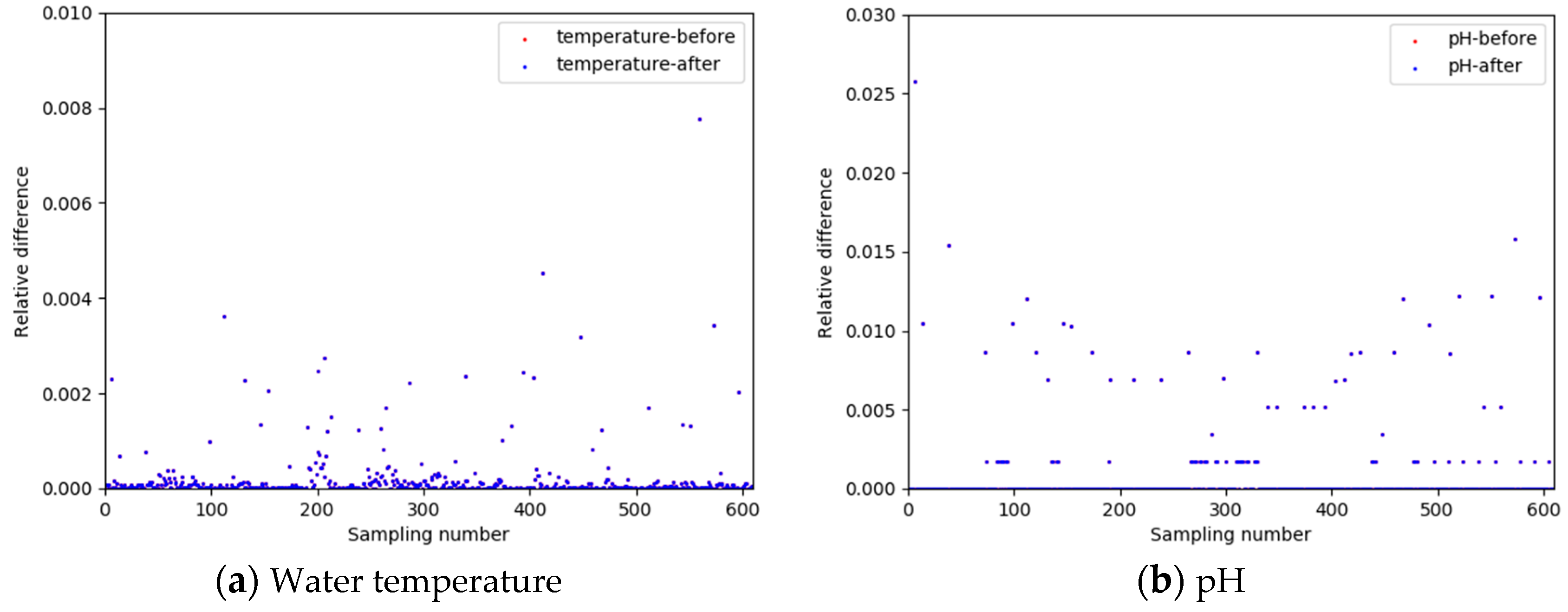
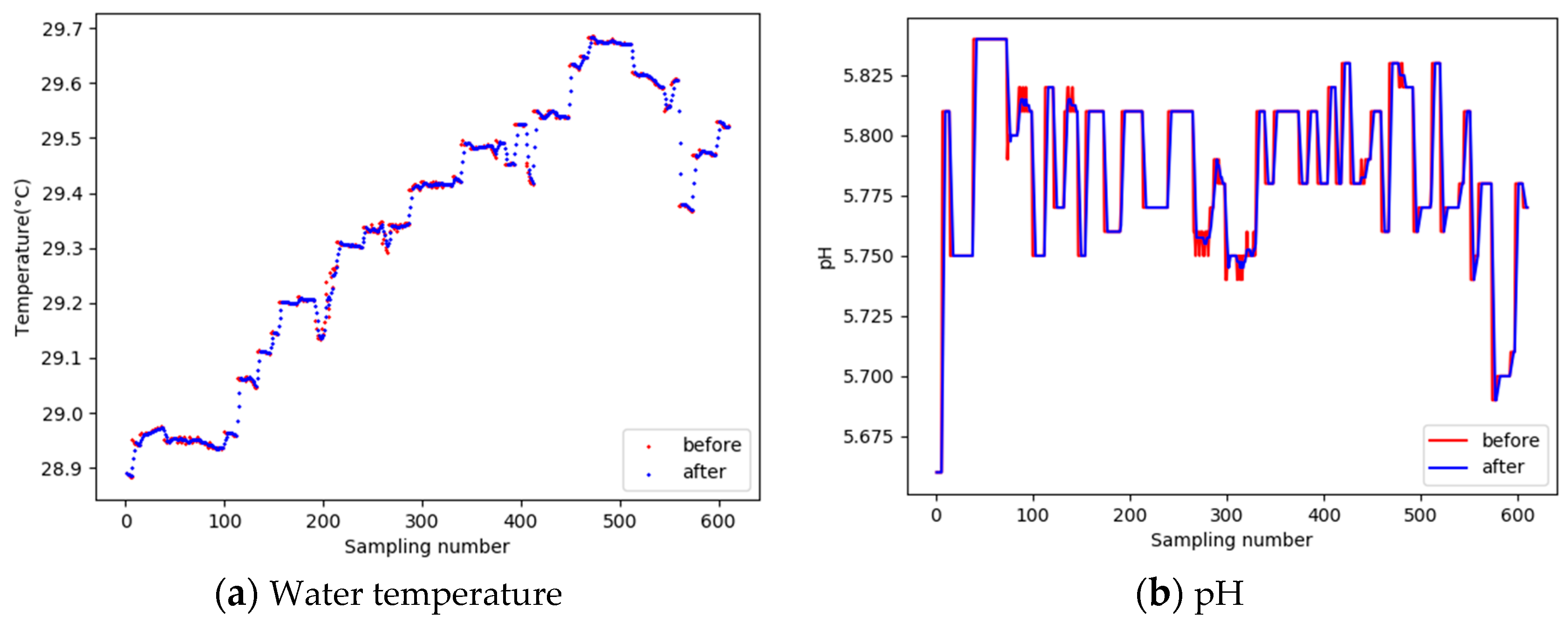
- The linear interpolation method and smoothing method are used to fill and correct the data sampled by the sensors, respectively. The moving average filter is used to denoise the data after filling and correcting.
- The influence factors of pH and water temperature are analyzed comprehensively. The correlation between water temperature, pH, and other water quality parameters is obtained by Pearson’s correlation coefficient method, which can be used as the input parameters of the model training.
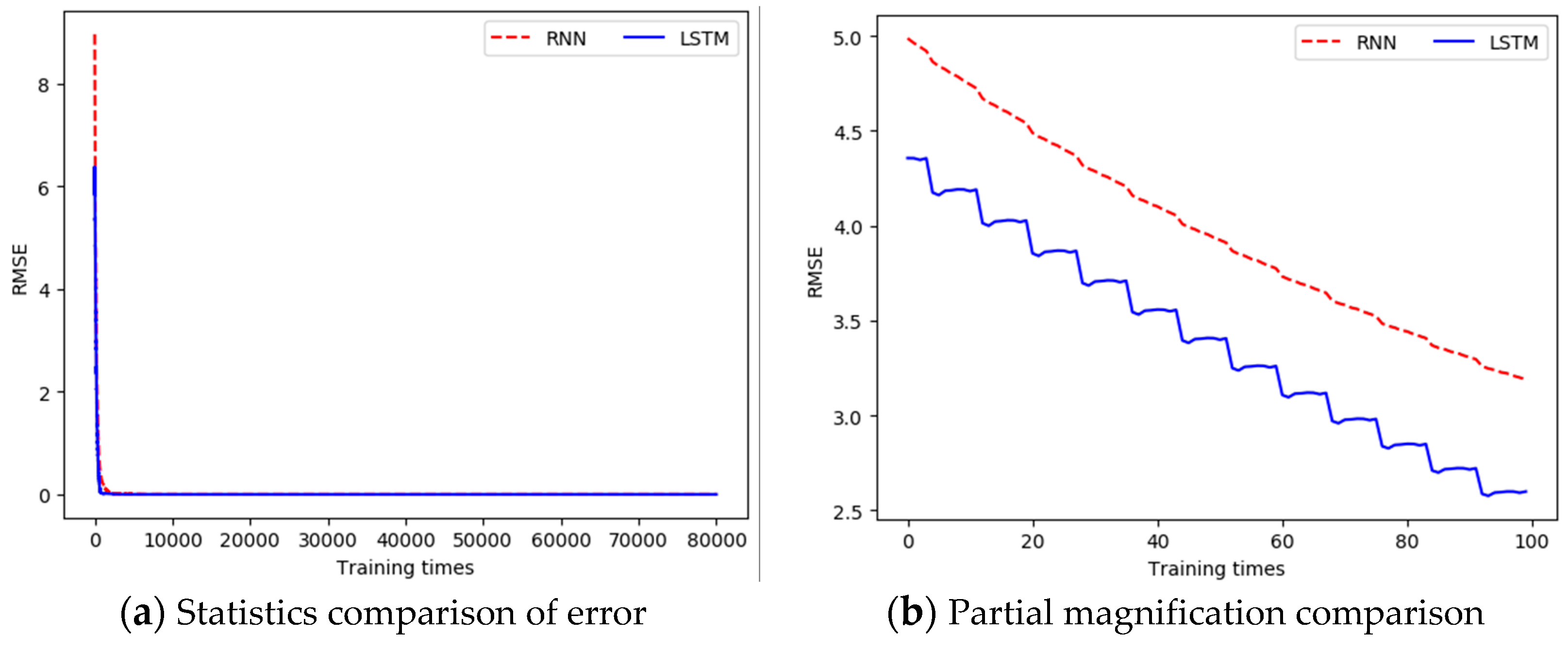
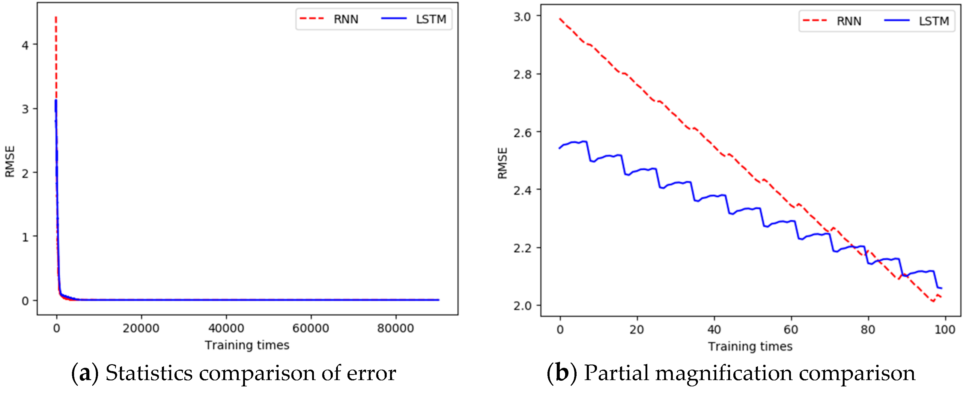
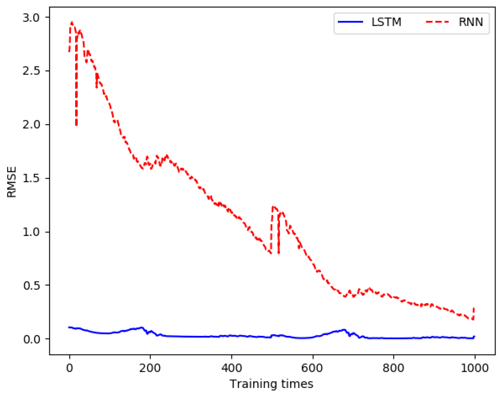
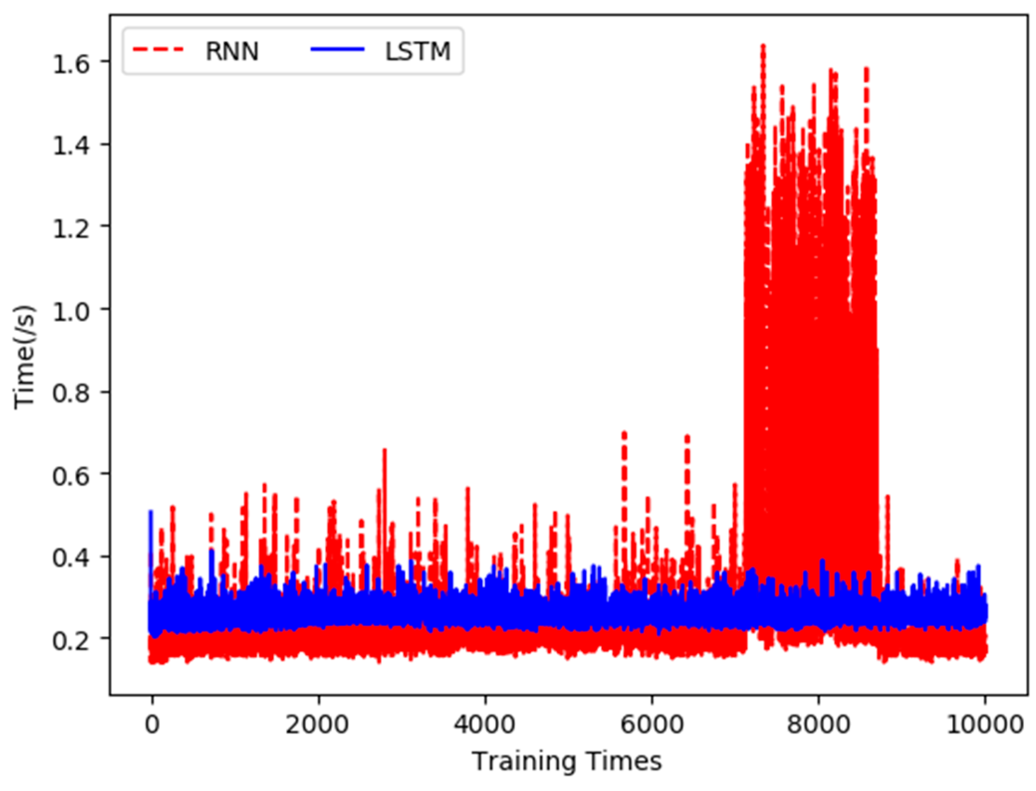
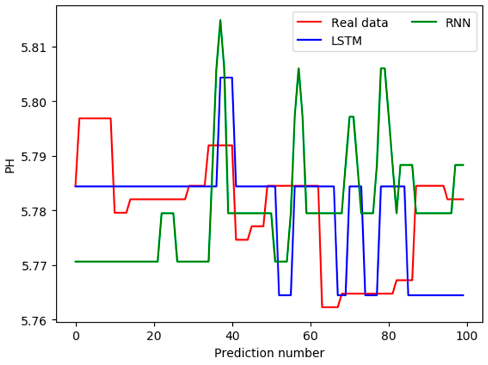
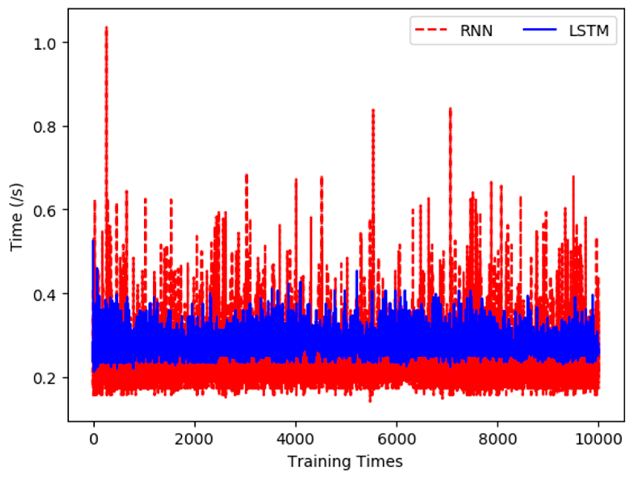
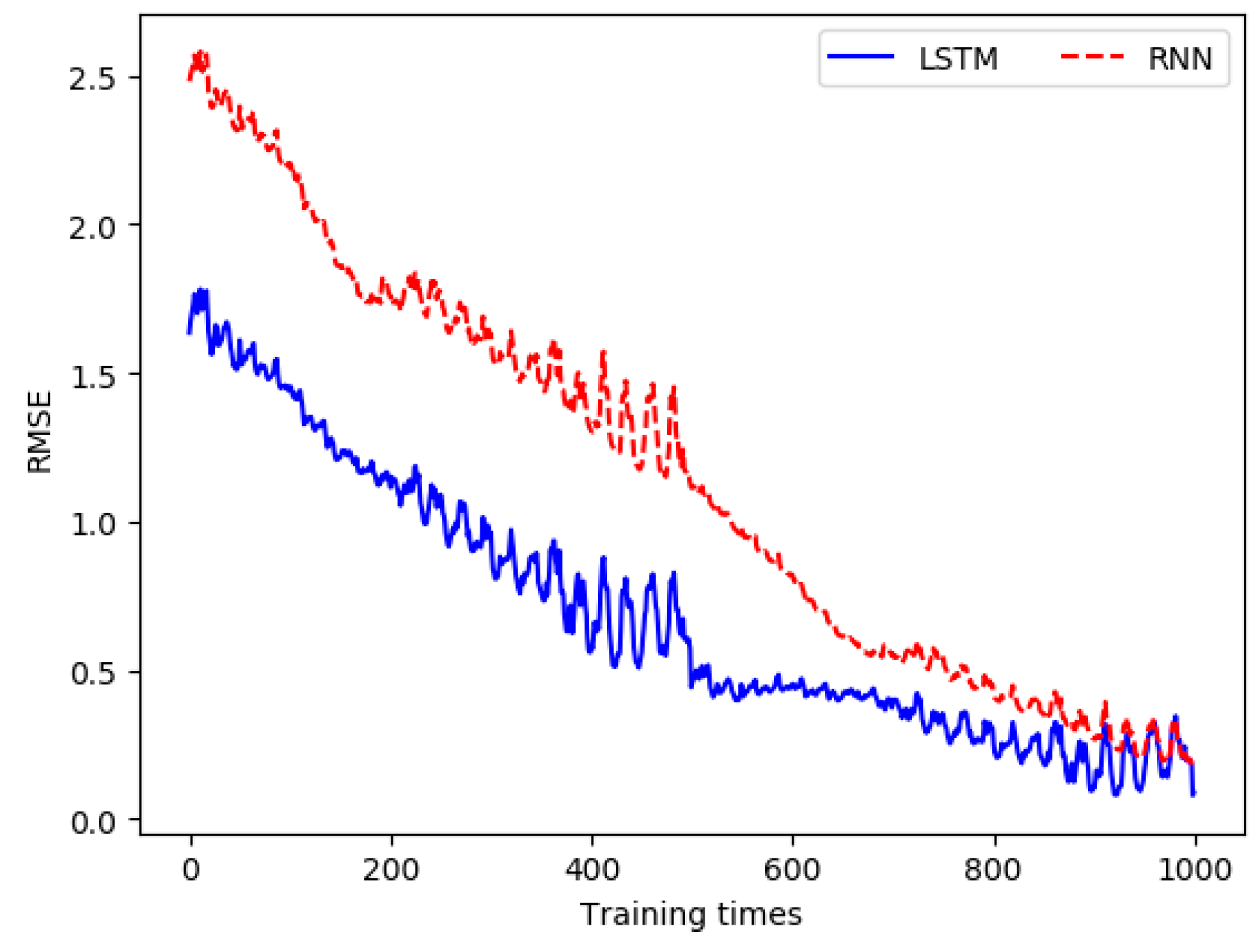
- Based on the pre-processed data and the correlation analysis results, a water quality prediction model based on a deep LSTM learning network is trained. Compared with the RNN based prediction model, the proposed prediction method can obtain higher prediction accuracy with less time.
2. Materials and Methods
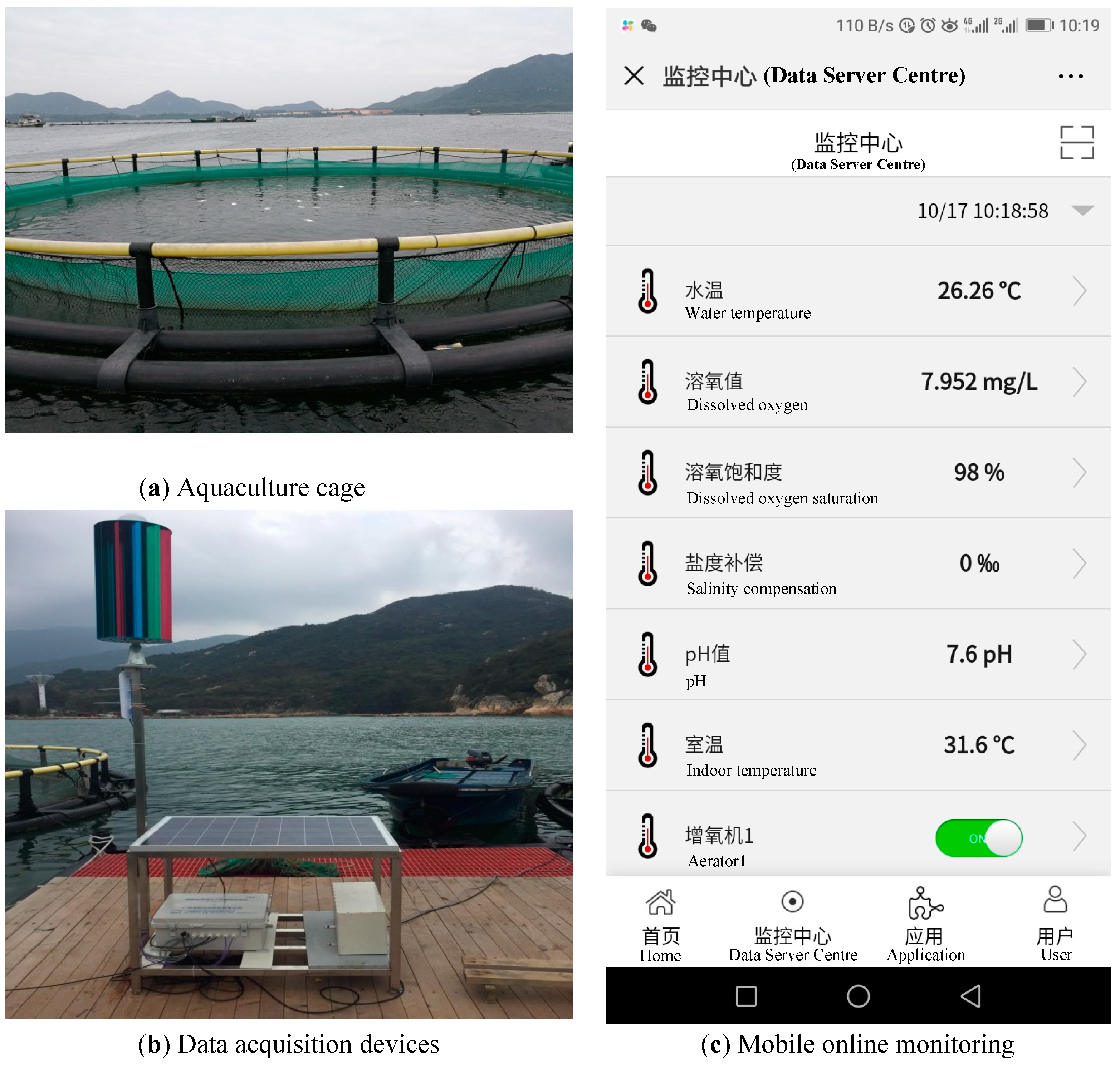
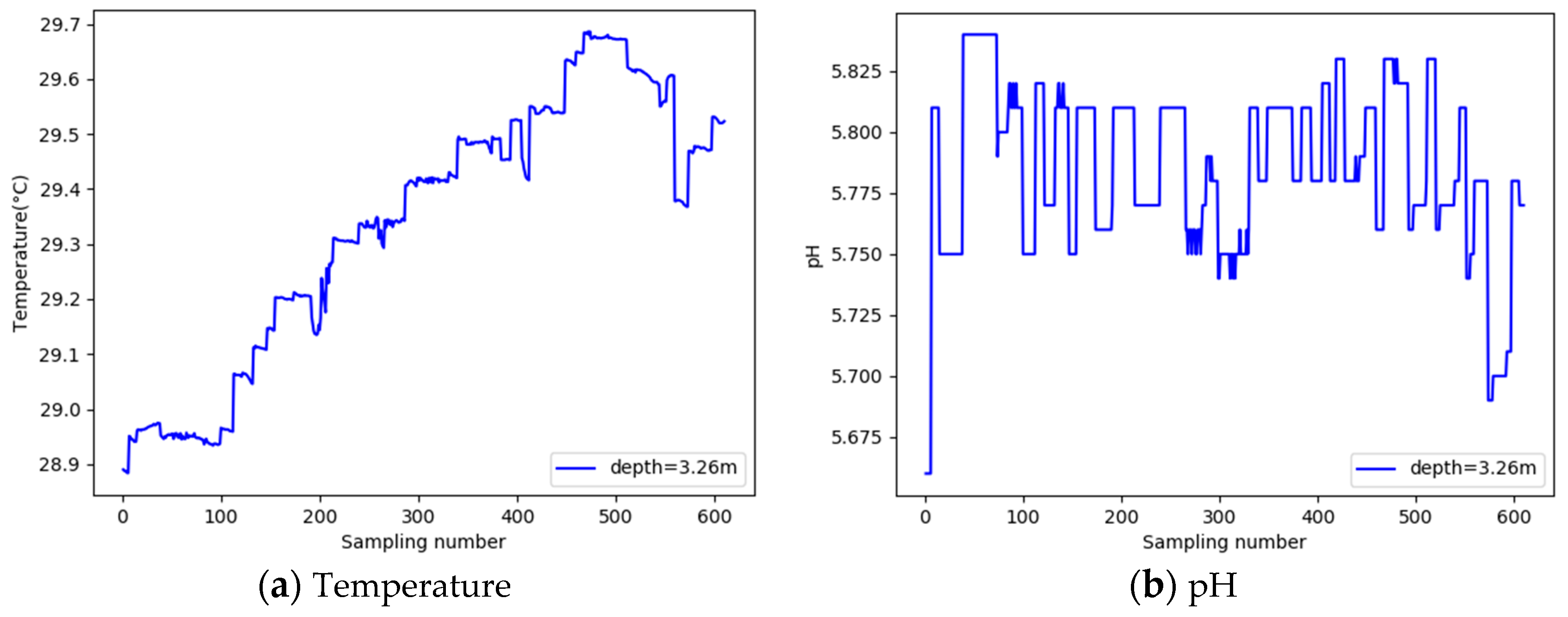
2.1. Data Acquisition
2.2. Data Preprocessing
2.2.1. Data Filling and Correction
2.2.2. Moving Average Filtering
2.3. Correlation Analysis
2.4. The Proposed Prediction Model Based on LSTM Deep Learning
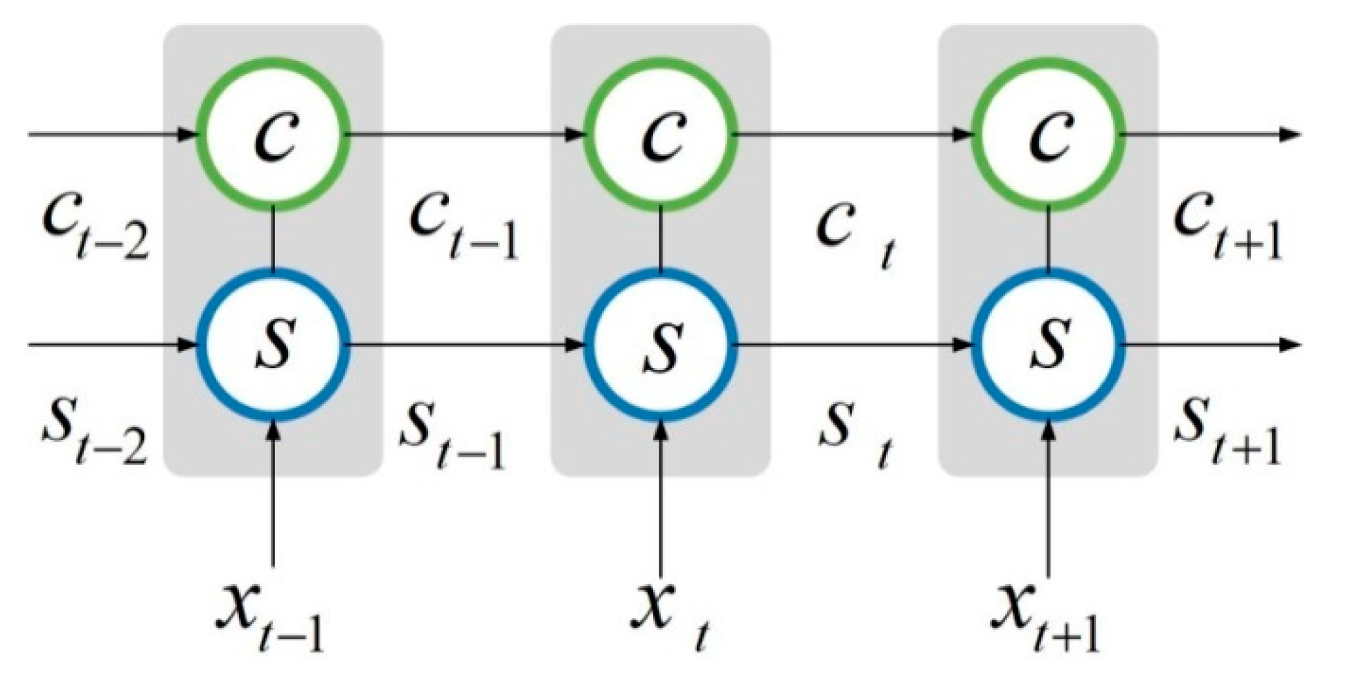
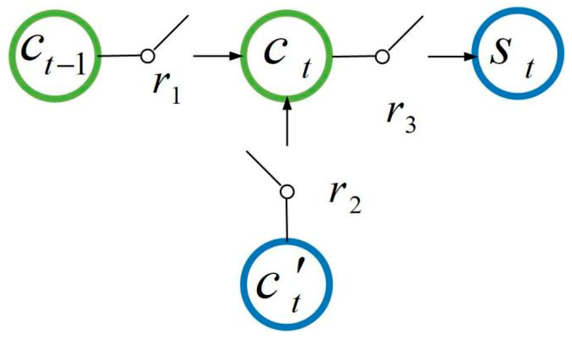
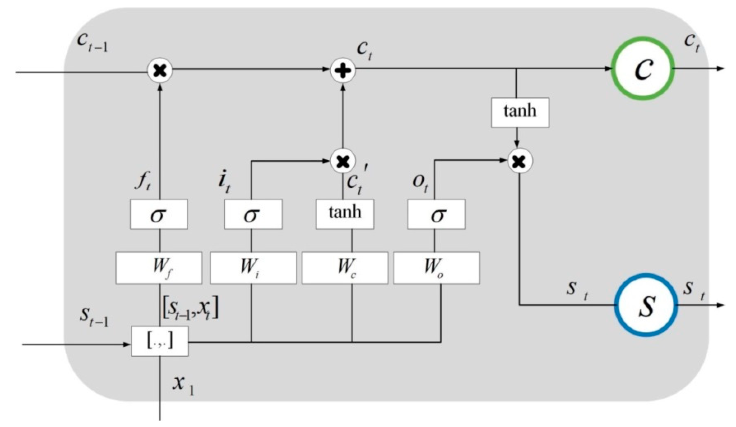
2.4.1. LSTM Deep Learning Network
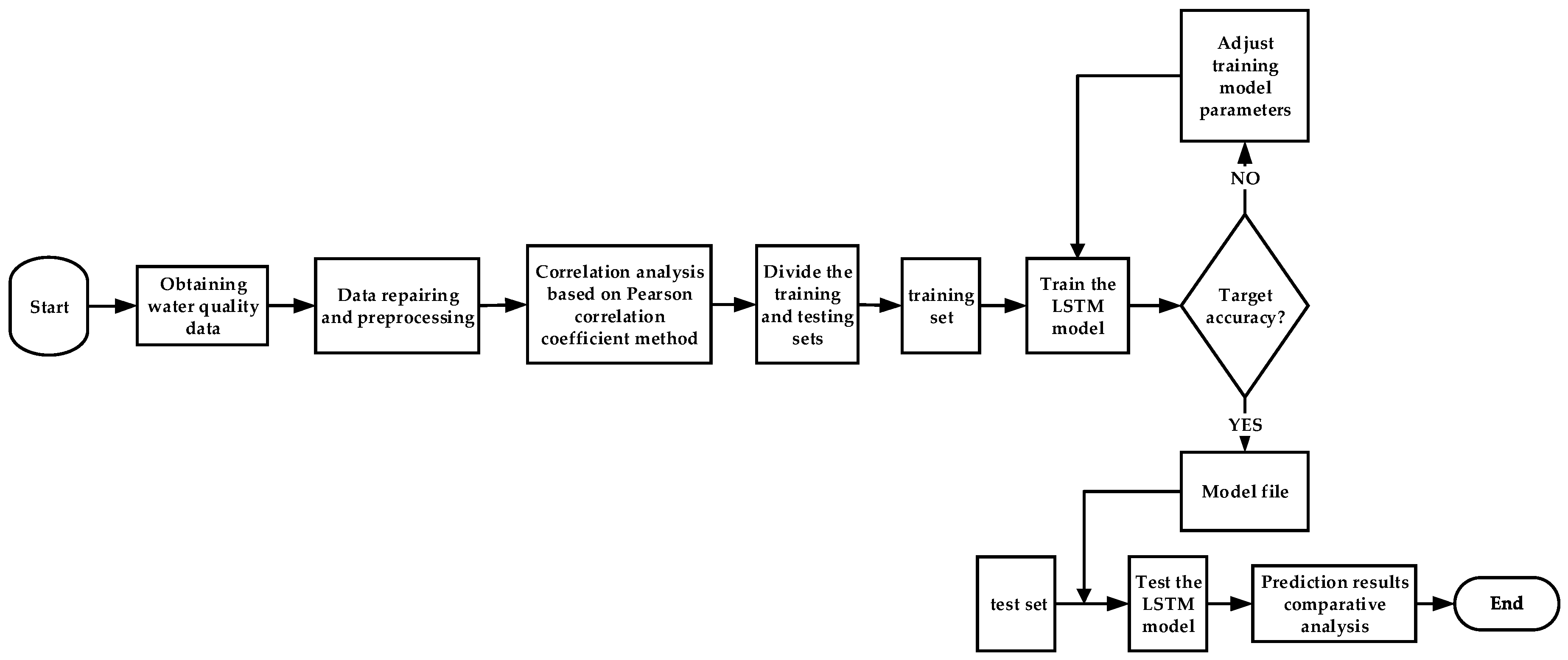
2.4.2. Construction of a Water Temperature and pH Prediction Model Based on the LSTM Deep Network
3. Results and Discussions
3.1. Experiments and Analysis of Data Preprocessing
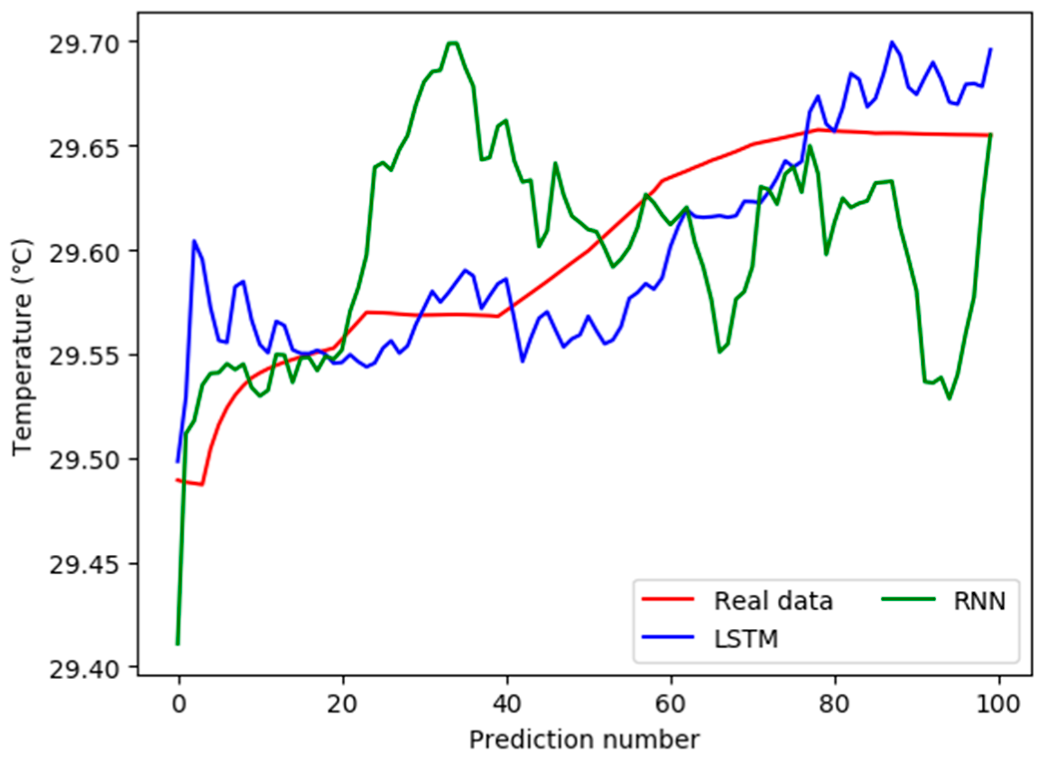
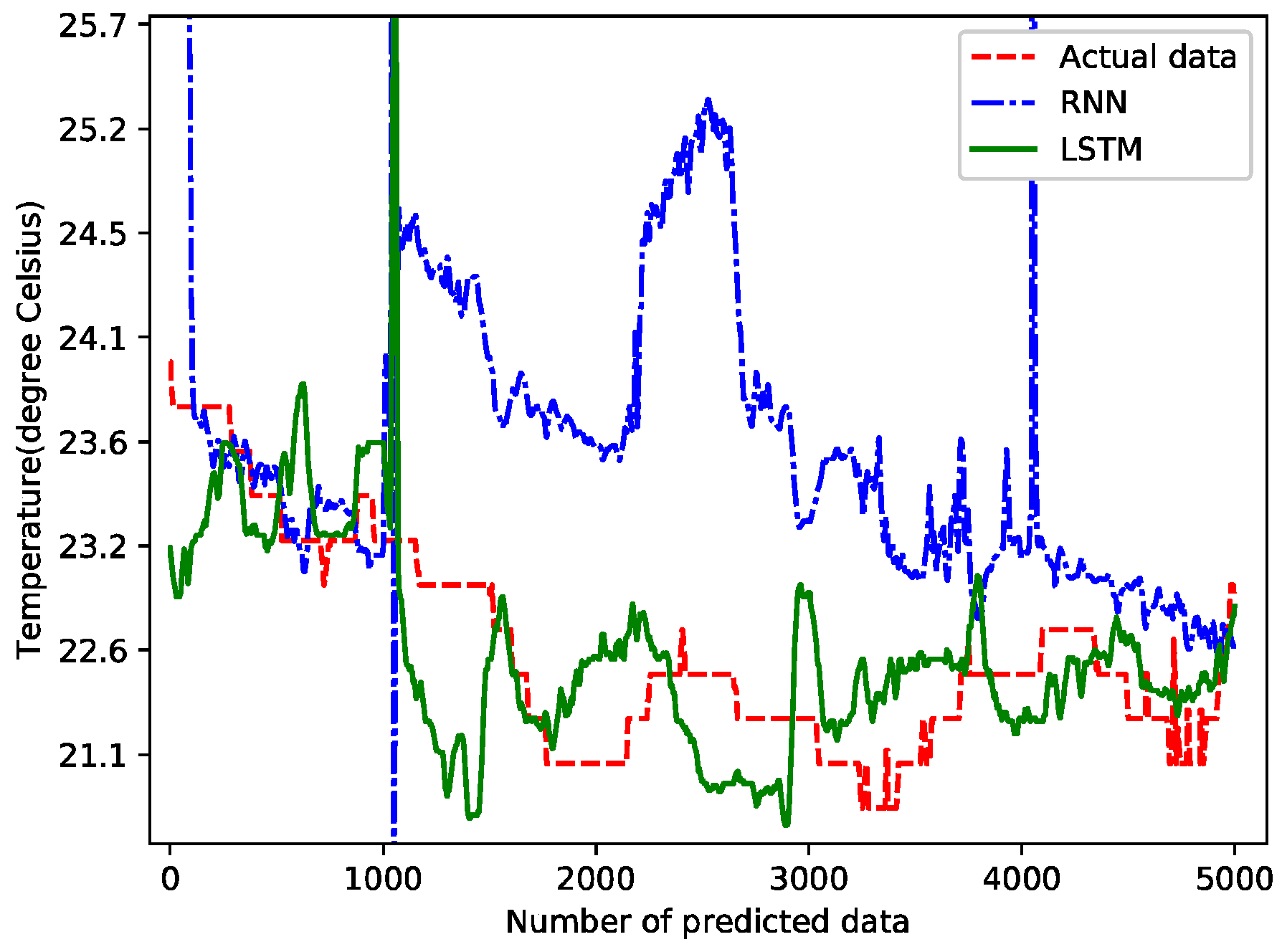
3.2. Experiments and Analysis of Water Temperature Short-term Prediction
3.2.1. The Prediction of Water Temperature
3.2.2. Time Complexity Analysis
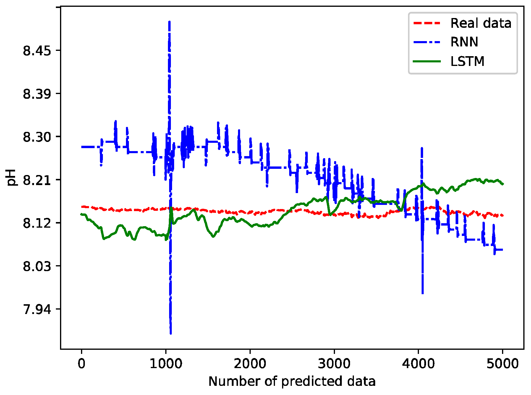
3.3. Experiments and Analysis of pH Short-Term Prediction
3.3.1. Prediction of pH Values
3.3.2. Time Complexity Analysis
3.4. Long-Term Prediction of Water Temperature and pH
3.5. Discussions
4. Conclusions
Author Contributions
Funding
Conflicts of Interest
References
- Liao, X.; Huang, H.; Dai, M.; Lin, Q. The synthetic evaluation and early warning of aquaculture area in Dapeng Cove of Daya Bay, South China Sea. In Proceedings of the 5th International Conference on Bioinformatics and Biomedical Engineering, Wuhan, China, 10–12 May 2011; pp. 1–5. [Google Scholar]
- Liu, S.; Xu, L.; Li, D. Prediction of dissolved oxygen content in river crab culture based on least squares support vector regression optimized by improved particle swarm optimization. Comput. Electron. Agric. 2013, 95, 82–91. [Google Scholar] [CrossRef]
- Xie, B.; Ding, Z.; Wang, X. Impact of the intensive shrimp farming on the water quality of the adjacent coastal creeks from Eastern China. Mar. Pollut. Bull. 2004, 48, 543–553. [Google Scholar]
- Yang, Q.; Tan, B.; Dong, X.; Chi, S.; Liu, H. Effects of different levels of yucca schidigera extract on the growth and nonspecific immunity of pacific white shrimp (litopenaeus vannamei) and on culture water quality. Aquaculture 2015, 439, 39–44. [Google Scholar] [CrossRef]
- Boyd, C.E.; Tucker, C.S. Pond Aquaculture Water Quality Management; Springer Science & Business Media: New York, NY, USA, 1998. [Google Scholar]
- Jin, C.; Liu, H.; Zhou, A. Functional dependency and conditional constraint based data repair. J. Softw. 2016, 27, 1671–1684. [Google Scholar]
- Zhang, X.; Hu, N.; Cheng, Z.; Zhong, H. Vibration data recovery based on compressed sensing. Acta Phys. Sin. 2014, 63, 119–128. [Google Scholar]
- Xu, W.; Zhu, X.; Liu, Z. Research on the key technology of urban multi-source traffic data analysis and processing. J. Zhejiang Univ. Technol. 2018, 46, 305–315. [Google Scholar]
- Singh, V.K.; Rai, A.K.; Kumar, M. Sparse data recovery using optimized orthogonal matching pursuit for WSNs. Proced. Comput. Sci. 2017, 109, 210–216. [Google Scholar] [CrossRef]
- Jakóbczak, D.J. 2D and 3D curve modeling-multidimensional data recovery. Eng. Appl. Artif. Intell. 2017, 64, 208–212. [Google Scholar] [CrossRef]
- Zhang, W.; Yan, H.; Wang, J. Research on data noise reduction method based on modified PCNN. Mach. Des. Manuf. 2015, 2, 25–28. [Google Scholar]
- Pan, Y.; Li, D.; Tong, Y. Noise reducing of data based on wavelet technology. J. Mach. Des. 2006, 1, 31–41. [Google Scholar]
- Wang, D.; Miao, D.; Wang, R. A new method of EEG classification with feature extraction based on wavelet packet decomposition. Acta Electron. Sin. 2013, 41, 193–198. [Google Scholar] [CrossRef]
- Li, Y.; Du, W.; Ye, P.; Liu, C. Wavelet leaders multifractal features extraction and performance analysis for vibration signals. J. Mech. Eng. 2013, 49, 60–65. [Google Scholar] [CrossRef]
- Perelli, A.; De Marchi, L.; Marzani, A.; Speciale, N. Frequency warped cross-wavelet multiresolution analysis of guided waves for impact localization. Signal Process. 2014, 96, 51–62. [Google Scholar] [CrossRef]
- Fabijańczyk, P.; Zawadzki, J.; Wojtkowska, M. Geostatistical study of spatial correlations of lead and zinc concentration in urban reservoir. Study case Czerniakowskie Lake, Warsaw, Poland. Open Geosci. 2016, 8, 484–492. [Google Scholar] [CrossRef]
- Zhu, Y.; Nan, C. Dynamic forecast of regional groundwater level based on grey Markov chain model. Chin. J. Geotech. Eng. 2011, 33, 71–75. [Google Scholar]
- Xue, P.; Feng, M.; Xing, X. Water quality prediction model based on Markov chain improving gray neural network. Eng. J. Wuhan Univ. 2012, 45, 319–324. [Google Scholar]
- Yue, Y.; Li, T. The application of a fuzzy-set theory based Markov model in the quantitative prediction of water quality. J. Basic Sci. Eng. 2011, 19, 231–242. [Google Scholar]
- Abaurrea, J.; Asín, J.; Cebrián, A.C.; García-Vera, M.A. Trend analysis of water quality series based on regression models with correlated errors. J. Hydrol. 2011, 400, 341–352. [Google Scholar] [CrossRef]
- Zhu, L.; Guan, D.; Wang, Y.; Liu, G.; Kang, K. Fuzzy comprehensive evaluation of water eutrophication of typical lakes and reservoirs. Resour. Environ. Yangtze Basin 2012, 21, 1131–1136. [Google Scholar]
- Tu, Z.; Han, T.; Chen, X.; Wu, R.; Wang, D. Thecommunity structure and diversity of macrobenthos in Linshui Xincungang and Li’ angang Seagrass Special Protected Area, Hainan. Mar. Environ. Sci. 2016, 35, 41–48. [Google Scholar]
- Yang, X.; Jin, W. GIS-based spatial regression and prediction of water quality in river networks: A case study in Iowa. J. Environ. Manag. 2010, 91, 1943–1951. [Google Scholar] [CrossRef] [PubMed]
- Zou, S.; Yu, Y. A dynamic factor model for multivariate water quality time series with trends. J. Hydrol. 1996, 178, 381–400. [Google Scholar] [CrossRef]
- Wu, J.; Lu, J.; Wang, J. Application of chaos and fractal models to water quality time series prediction. Environ. Model. Softw. 2009, 24, 632–636. [Google Scholar] [CrossRef]
- Chan, S.; Thoe, W.; Lee, J.H.W. Real-time forecasting of Hong Kong beach water quality by 3D deterministic model. Water Res. 2013, 47, 1631–1647. [Google Scholar] [CrossRef] [PubMed]
- Feng, T.; Wang, C.; Hou, J.; Wang, P.; Liu, Y.; Dai, Q. Effect of inter-basin water transfer on water quality in an urban lake: A combined water quality index algorithm and biophysical modelling approach. Ecol. Indic. 2018, 92, 61–71. [Google Scholar] [CrossRef]
- Li, Z.; Jiang, Y.; Yue, J. An improved gray model for aquaculture water quality prediction. Intell. Autom. Soft Comput. 2012, 18, 557–567. [Google Scholar] [CrossRef]
- Cho, S.; Lim, B.; Jung, J. Factors affecting algal blooms in a man-made lake and prediction using an artificial neural network. Measurement 2014, 53, 224–233. [Google Scholar] [CrossRef]
- Yang, F.; Li, G.; Zhang, B.; Deng, S. Study on oxygen increasing effect of spirulina in aquaculture sewage and a prediction model. Chin. J. Environ. Eng. 2012, 6, 3001–3006. [Google Scholar]
- Xu, L.; Liu, S. Study of short-term water quality prediction model based on wavelet neural network. Math. Comput. Model. 2013, 58, 807–813. [Google Scholar] [CrossRef]
- Tan, G.; Yan, J.; Gao, C. Prediction of water quality time series data based on least squares support vector machine. Proced. Eng. 2012, 31, 1194–1199. [Google Scholar] [CrossRef]
- Singh, K.P.; Basant, N.; Gupta, S. Support vector machines in water quality management. Anal. Chim. Acta 2011, 703, 67–68. [Google Scholar] [CrossRef] [PubMed]
- Preis, A.; Ostfeld, A. A coupled model tree-genetic algorithm scheme for flow and water quality predictions in watersheds. J. Hydrol. 2008, 349, 364–375. [Google Scholar] [CrossRef]
- Gers, F.A.; Schmidhuber, J.; Cummins, F. Learning to forget: Continual prediction with LSTM. Neural Comput. 2000, 12, 2451–2471. [Google Scholar] [CrossRef] [PubMed]
- Graves, A.; Mohamed, A.R.; Hinton, G. Speech recognition with deep recurrent neural networks. In Proceedings of the IEEE International Conference on Acoustics, Speech and Signal Processing, Vancouver, BC, Canada, 26–31 May 2013; pp. 6645–6649. [Google Scholar]
- Xu, L.; Liu, S. Water quality prediction model based on APSO-WLSSVR. Shandong Univ. Eng. Sci. 2012, 42, 80–86. [Google Scholar] [CrossRef]
- Lee, R.J.; Nicewander, W.A. Thirteen ways to look at the correlation coefficient. Am. Stat. 1988, 42, 59–66. [Google Scholar]
- Chen, Y.; Cheng, Q.; Fang, X.; Yu, H.; Li, D. Principal component analysis and long short-term memory neural network for predicting dissolved oxygen in water for aquaculture. Trans. Chin. Soc. Agric. Eng. 2018, 34, 183–191. [Google Scholar]
- Hu, Z.; Bai, Y.; Zhao, Y.; Xie, M. Adaptive and blind wideband spectrum sensing scheme using singular value decomposition. Wirel. Commun. Mob. Comput. 2017, 2017, 3279452. [Google Scholar] [CrossRef]
- Hu, Z.; Bai, Y.; Huang, M.; Xie, M.; Zhao, Y. A self-adaptive progressive support selection scheme for collaborative wideband spectrum sensing. Sensors 2018, 18, 3011. [Google Scholar] [CrossRef]


| Conductivity | Salinity | Chlorophyll | Turbidity | Water Temperature | pH | Dissolved Oxygen | |
|---|---|---|---|---|---|---|---|
| pH | −0.9754 | 0.866538 | −0.51448 | −0.04556 | −0.97497 | 1 | 0.197046 |
| Water Temperature | 0.999459 | −0.91028 | 0.565859 | 0.202542 | 1 | −0.97497 | 0.791544 |
| Training Time | MAE | RMSE | MAPE | |||||||||
|---|---|---|---|---|---|---|---|---|---|---|---|---|
| Temperature | pH | Temperature(°C) | pH | Temperature | pH | |||||||
| LSTM | RNN | LSTM | RNN | LSTM | RNN | LSTM | RNN | LSTM | RNN | LSTM | RNN | |
| 1000 | 0.0149 | 0.0175 | 0.0415 | 0.053 | 0.0479 | 0.111 | 0.113 | 0.120 | 0.0455 | 0.0692 | 0.0168 | 0.0239 |
| 2000 | 0.013 | 0.0156 | 0.0182 | 0.0203 | 0.0222 | 0.0285 | 0.0389 | 0.0457 | 0.0362 | 0.0350 | 0.0032 | 0.0104 |
| 5000 | 0.0121 | 0.0143 | 0.00739 | 0.00824 | 0.0168 | 0.0189 | 0.0039 | 0.0051 | 0.0323 | 0.0337 | 0.0013 | 0.0038 |
| 10,000 | 0.0105 | 0.0132 | 0.00274 | 0.00325 | 0.0145 | 0.0155 | 0.0025 | 0.0031 | 0.0289 | 0.0326 | 0.0012 | 0.0023 |
| Technical Parameters of Sensors | The Type of Sensors | |||||
|---|---|---|---|---|---|---|
| Salinity | Chlorophyll | Turbidity | Water Temperature | pH | Dissolved Oxygen | |
| Range ability | 0 ~ 100PSU | 0 ~ 400 ug/L | 0.1 ~ 1000 NTU | −10 ~ 60°C | 0 ~ 14 | 0 ~ 20.00 mg/L |
| Accuracy | ±1.5% F.S. | ±3% F.S. | ±1.0 NTU | ±0.2°C | ±0.01 | ±1.5%F.S. |
| Group Number | The Deviations between the Real Values and the Predicted Values | |||||||
|---|---|---|---|---|---|---|---|---|
| LSTM | RNN | LSTM | RNN | LSTM | RNN | LSTM | RNN | |
| 1 | 0.132949 | 3.959442 | 0.541791 | 0.414951 | 2.540453 | 0.056431 | 0.198738 | 0.189815 |
| 2 | 0.400642 | 3.114111 | 0.356221 | 0.503157 | 2.797719 | 0.028507 | 0.147363 | 0.436588 |
| 3 | 1.036029 | 3.069812 | 0.252005 | 0.396319 | 3.00332 | 0.417664 | 0.333328 | 0.013683 |
| 4 | 0.961058 | 2.934413 | 0.409308 | 0.658454 | 2.841458 | 0.820384 | 0.482137 | 0.259189 |
| 5 | 0.728714 | 2.624992 | 0.300582 | 0.833992 | 2.502212 | 0.669596 | 0.216224 | 1.036307 |
| 6 | 0.519411 | 2.46428 | 0.010955 | 1.187961 | 1.915524 | 0.46367 | 0.146241 | 0.724474 |
| 7 | 0.459601 | 2.312542 | 0.244412 | 1.439206 | 1.776256 | 0.124387 | 0.371641 | 0.489075 |
| 8 | 0.768172 | 2.280364 | 0.471358 | 1.513481 | 1.586839 | 0.408896 | 0.699684 | 0.587774 |
| 9 | 0.78813 | 2.199178 | 0.343911 | 1.485762 | 1.655596 | 0.205522 | 0.63025 | 0.558739 |
| 10 | 0.505946 | 2.333197 | 0.473716 | 1.770735 | 1.412733 | 0.141486 | 0.368266 | 0.533711 |
| 11 | 0.246733 | 2.372123 | 0.616469 | 1.727489 | 0.960963 | 0.400867 | 0.447675 | 0.3642 |
| 12 | 0.059172 | 2.336197 | 0.754278 | 1.390779 | 0.702773 | 0.360609 | 0.683729 | 0.358777 |
| 13 | 0.232154 | 2.019102 | 0.690577 | 1.144995 | 0.528385 | 0.320189 | 0.98381 | 0.349546 |
| 14 | 0.010727 | 2.111242 | 0.300113 | 0.267601 | 0.632107 | 0.791274 | 0.86618 | 0.785739 |
| 15 | 0.280356 | 2.448614 | 0.45345 | 0.289334 | 0.658988 | 1.088531 | 0.561477 | 1.077822 |
| 16 | 0.303246 | 2.125633 | 0.595648 | 0.666767 | 0.670855 | 1.459331 | 0.49732 | 1.390808 |
| 17 | 0.289681 | 2.111117 | 0.588843 | 1.139716 | 0.671857 | 1.98203 | 0.668225 | 2.270634 |
| 18 | 0.236164 | 2.268004 | 0.203486 | 0.983571 | 0.698048 | 1.908593 | 0.831318 | 2.285945 |
| 19 | 0.276489 | 2.086995 | 1.50439 | 1.087927 | 0.694925 | 1.510539 | 0.684134 | 2.234941 |
| 20 | 0.394135 | 2.125502 | 1.791799 | 1.889873 | 0.561602 | 1.438296 | 0.460814 | 2.447277 |
| 21 | 0.412513 | 2.02414 | 2.644721 | 0.006956 | 0.559784 | 1.203195 | 0.446673 | 2.207668 |
| 22 | 0.344401 | 1.536572 | 9.840927 | 3.26874 | 0.56474 | 0.458536 | 0.649647 | 1.790473 |
| 23 | 0.467034 | 1.227761 | 12.08877 | 11.93078 | 0.458013 | 0.468914 | 0.662479 | 1.431288 |
| 24 | 0.567662 | 0.786095 | 5.92811 | 2.601457 | 0.320005 | 0.58208 | 0.633802 | 0.481562 |
| 25 | 0.541791 | 0.414951 | 3.764784 | 0.738845 | 0.152873 | 0.284062 | 1.006936 | 0.195481 |
| Group Number | The Deviations between the Real Values and the Predicted Values | |||||||
|---|---|---|---|---|---|---|---|---|
| LSTM | RNN | LSTM | RNN | LSTM | RNN | LSTM | RNN | |
| 1 | 0.630802 | 2.136396 | 2.855522 | 0.765329 | 1.496367 | 1.962419 | 2.198166 | 1.002551 |
| 2 | 0.63822 | 2.079181 | 2.614542 | 0.006417 | 0.648587 | 0.551713 | 2.401637 | 0.829339 |
| 3 | 0.600423 | 2.119937 | 2.505741 | 0.207085 | 0.4615 | 0.475682 | 2.107028 | 0.041945 |
| 4 | 0.626563 | 2.185643 | 2.340742 | 0.091206 | 0.263681 | 0.433036 | 1.462349 | 1.816386 |
| 5 | 1.477082 | 0.577829 | 2.309721 | 0.078737 | 0.091957 | 0.539806 | 0.884081 | 2.00253 |
| 6 | 1.383567 | 0.714821 | 3.950786 | 1.472333 | 0.194655 | 1.105872 | 0.674252 | 1.057834 |
| 7 | 1.337259 | 0.755719 | 2.171247 | 0.125621 | 0.645851 | 2.272947 | 1.068124 | 0.320677 |
| 8 | 1.402000 | 0.456464 | 2.064245 | 0.383645 | 1.085894 | 2.573101 | 1.260291 | 0.622556 |
| 9 | 1.549016 | 0.202762 | 1.961289 | 0.434519 | 1.270665 | 2.070847 | 1.561966 | 0.385598 |
| 10 | 1.626345 | 0.332107 | 2.175619 | 1.163942 | 0.914486 | 0.769215 | 0.590714 | 1.411085 |
| 11 | 0.694443 | 1.909472 | 3.731103 | 3.2055 | 1.015838 | 1.065162 | 0.527791 | 1.390929 |
| 12 | 0.717155 | 1.998789 | 7.108605 | 11.80848 | 1.230752 | 0.973677 | 0.424462 | 1.346182 |
| 13 | 0.733518 | 1.914349 | 9.976984 | 13.51213 | 1.277154 | 0.954261 | 0.307454 | 1.125405 |
| 14 | 0.718865 | 1.868381 | 10.86092 | 8.786944 | 1.320137 | 0.931954 | 0.236954 | 1.048285 |
| 15 | 0.700548 | 1.857634 | 8.690118 | 2.051635 | 1.388031 | 0.921659 | 0.19318 | 1.064826 |
| 16 | 0.702013 | 1.811576 | 3.038798 | 1.456259 | 1.454459 | 1.149511 | 0.289509 | 1.163951 |
| 17 | 0.655123 | 1.750345 | 2.099476 | 0.854766 | 1.514782 | 1.228984 | 0.363189 | 1.241873 |
| 18 | 0.615315 | 1.731200 | 1.680865 | 0.881667 | 1.593909 | 1.266734 | 0.449198 | 1.270074 |
| 19 | 0.596754 | 1.751700 | 1.390518 | 0.916591 | 1.741908 | 1.105982 | 0.543807 | 1.206676 |
| 20 | 1.745037 | 0.484228 | 1.026786 | 0.760142 | 1.967495 | 0.593296 | 0.648737 | 1.139885 |
| 21 | 1.751331 | 0.50235 | 0.747286 | 1.308068 | 1.675005 | 0.524874 | 0.784917 | 1.149215 |
| 22 | 1.649274 | 0.291042 | 0.516284 | 1.542153 | 1.290587 | 0.158633 | 0.573094 | 1.300818 |
| 23 | 1.929368 | 0.281699 | 0.112988 | 1.793935 | 1.27862 | 0.197551 | 0.714104 | 1.626713 |
| 24 | 2.386151 | 1.274894 | 0.426867 | 1.854815 | 1.726579 | 0.699496 | 0.608600 | 1.668695 |
| 25 | 2.720645 | 1.371820 | 0.886318 | 1.898942 | 1.855515 | 0.974336 | 0.574483 | 1.471081 |
| Training Times | MAE | RMSE | MAPE | |||||||||
|---|---|---|---|---|---|---|---|---|---|---|---|---|
| Temperature | pH | Temperature(°C) | pH | Temperature | pH | |||||||
| LSTM | RNN | LSTM | RNN | LSTM | RNN | LSTM | RNN | LSTM | RNN | LSTM | RNN | |
| 500 | 0.0421 | 0.0439 | 0.0042 | 0.0325 | 0.0519 | 0.5340 | 0.6236 | 1.0875 | 0.085 | 0.078 | 0.0092 | 0.0102 |
| 1000 | 0.0312 | 0.0424 | 0.0035 | 0.0052 | 0.0457 | 0.1451 | 0.3108 | 0.3254 | 0.052 | 0.065 | 0.0068 | 0.0073 |
© 2019 by the authors. Licensee MDPI, Basel, Switzerland. This article is an open access article distributed under the terms and conditions of the Creative Commons Attribution (CC BY) license (http://creativecommons.org/licenses/by/4.0/).
Share and Cite
Hu, Z.; Zhang, Y.; Zhao, Y.; Xie, M.; Zhong, J.; Tu, Z.; Liu, J. A Water Quality Prediction Method Based on the Deep LSTM Network Considering Correlation in Smart Mariculture. Sensors 2019, 19, 1420. https://doi.org/10.3390/s19061420
Hu Z, Zhang Y, Zhao Y, Xie M, Zhong J, Tu Z, Liu J. A Water Quality Prediction Method Based on the Deep LSTM Network Considering Correlation in Smart Mariculture. Sensors. 2019; 19(6):1420. https://doi.org/10.3390/s19061420
Chicago/Turabian StyleHu, Zhuhua, Yiran Zhang, Yaochi Zhao, Mingshan Xie, Jiezhuo Zhong, Zhigang Tu, and Juntao Liu. 2019. "A Water Quality Prediction Method Based on the Deep LSTM Network Considering Correlation in Smart Mariculture" Sensors 19, no. 6: 1420. https://doi.org/10.3390/s19061420
APA StyleHu, Z., Zhang, Y., Zhao, Y., Xie, M., Zhong, J., Tu, Z., & Liu, J. (2019). A Water Quality Prediction Method Based on the Deep LSTM Network Considering Correlation in Smart Mariculture. Sensors, 19(6), 1420. https://doi.org/10.3390/s19061420