VisNet: Deep Convolutional Neural Networks for Forecasting Atmospheric Visibility


Abstract
1. Introduction
2. Related Works
2.1. ANNs-Based Methods
2.2. Statistical Approaches
3. Methods
3.1. Model
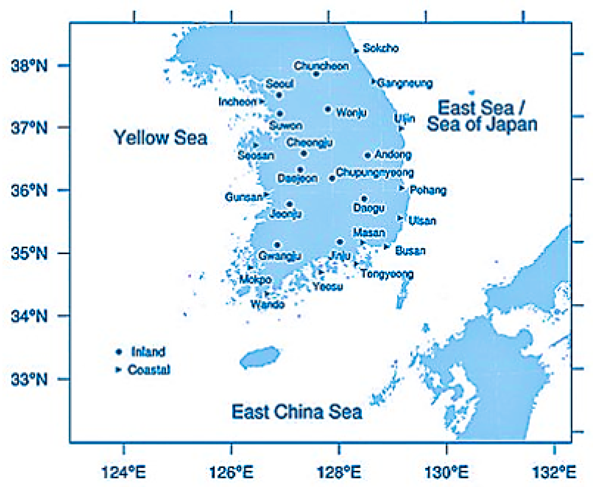
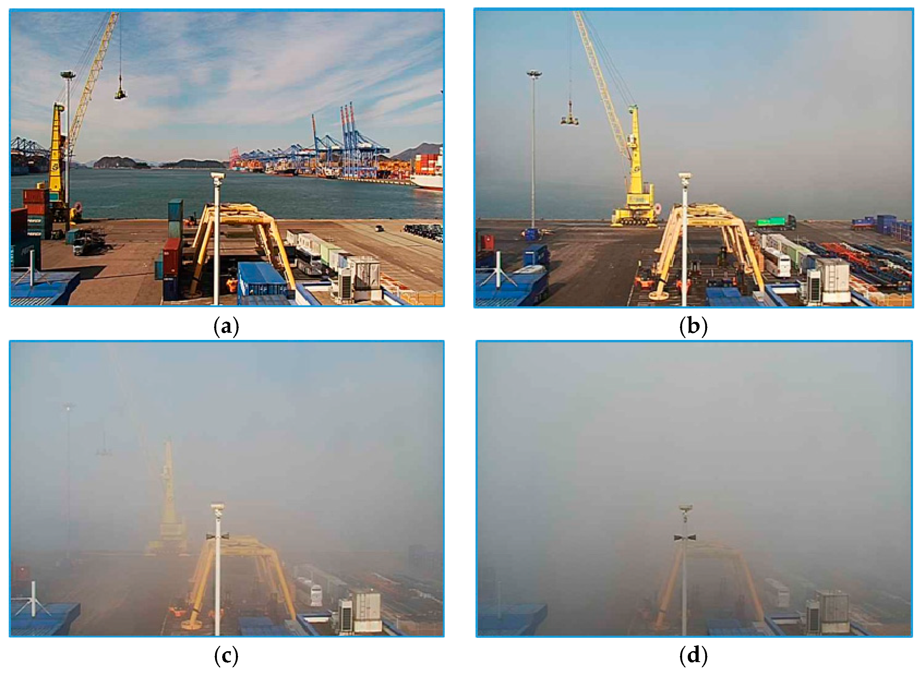
3.2. Datasets
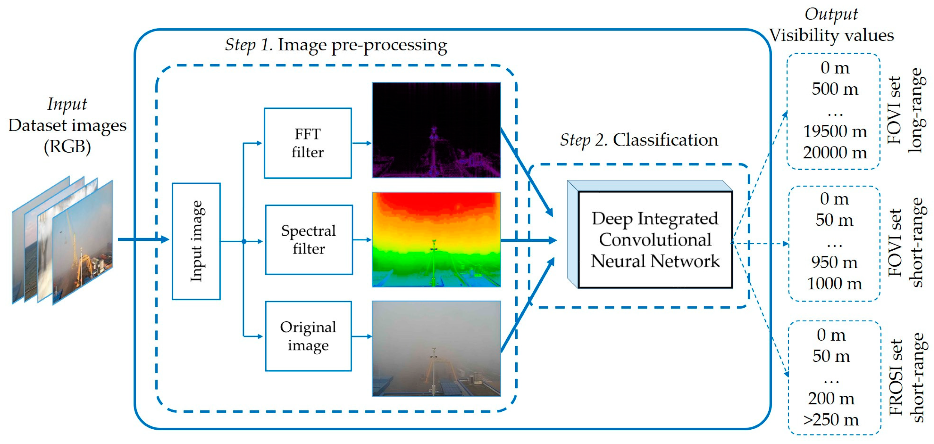
3.3. Image Pre-Processing
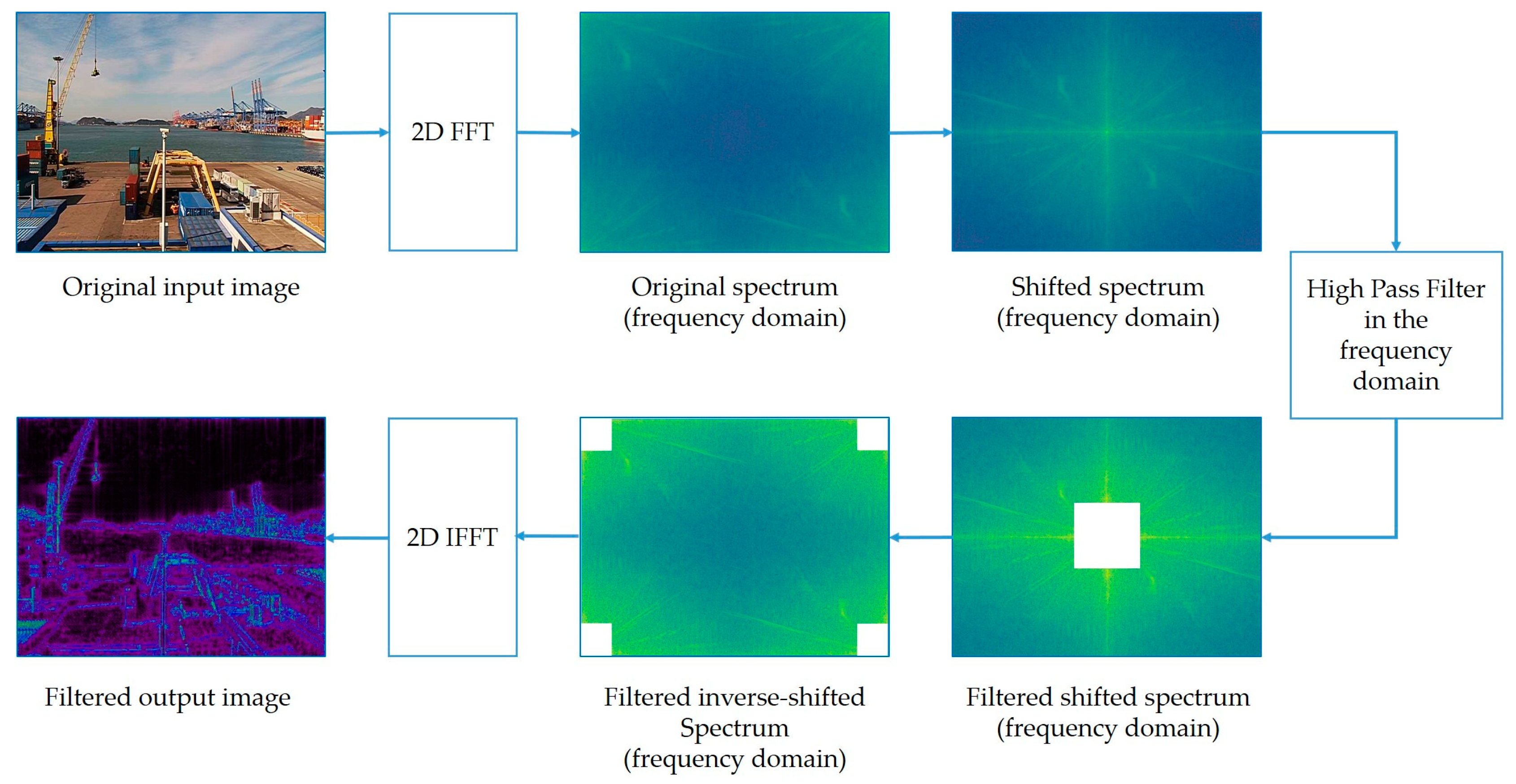
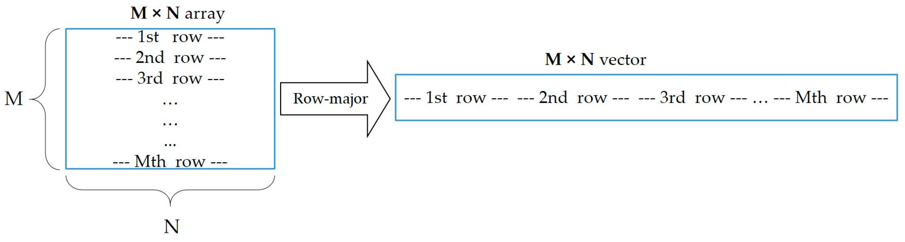
3.3.1. FFT-Based Filter
- For each row of f (m, n), performing a 1D FFT for each value of m;
- For each column, on the resulting values, performing a 1D FFT in the opposite direction.
- M 1D transforms over rows (each row having N instances);
- N 1D transforms over columns (each column having M instances).
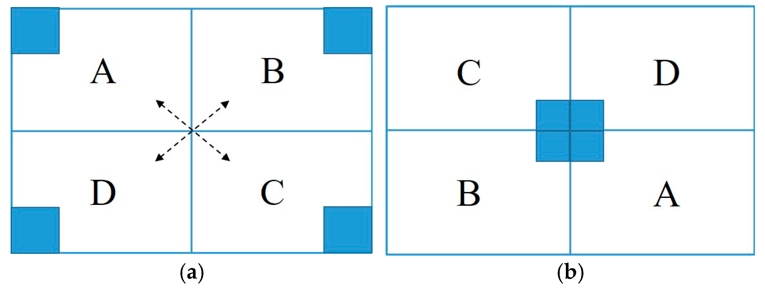
3.3.2. Spectral Filter
3.4. Classification
4. Experimental Results and Discussion
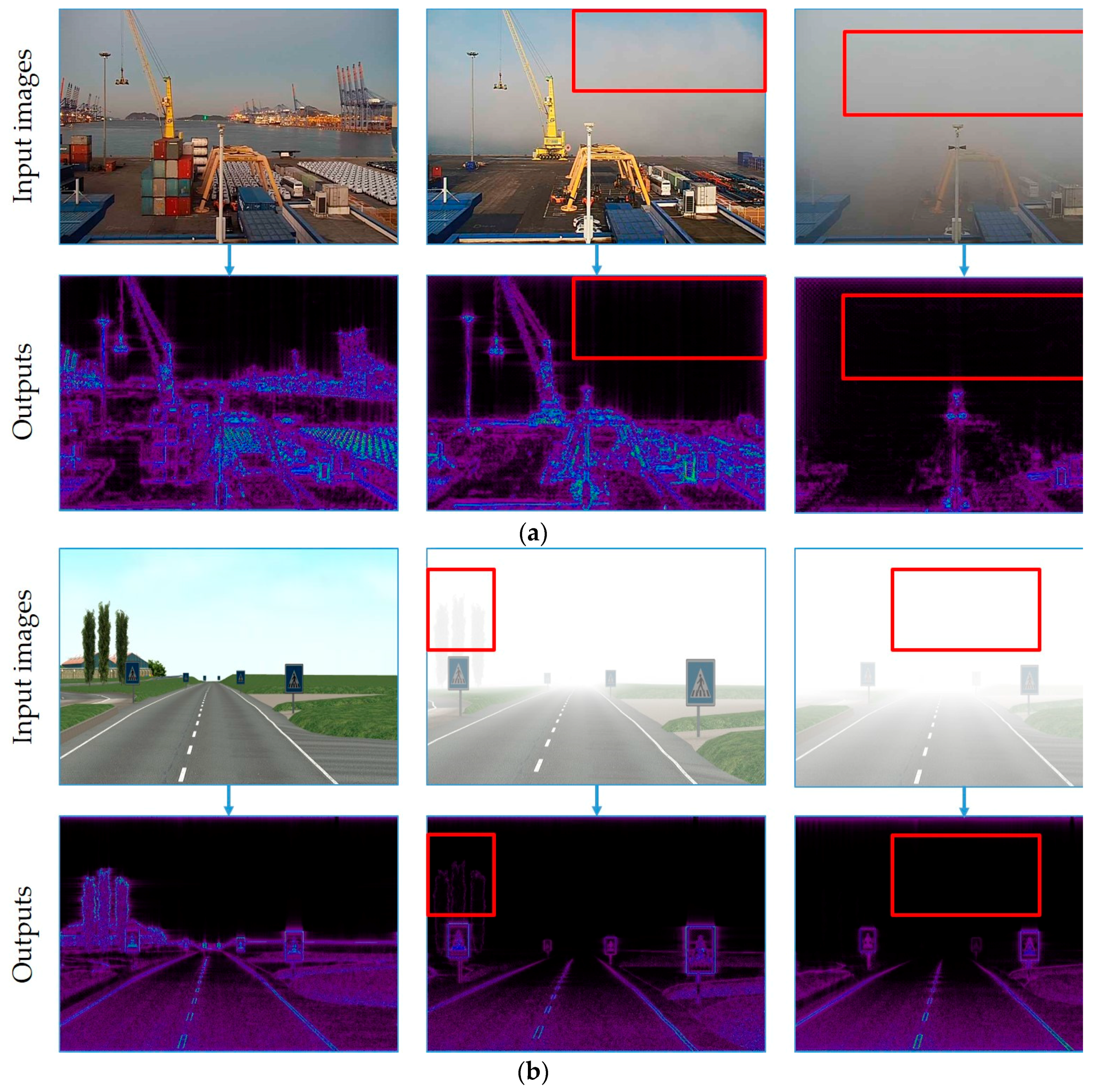
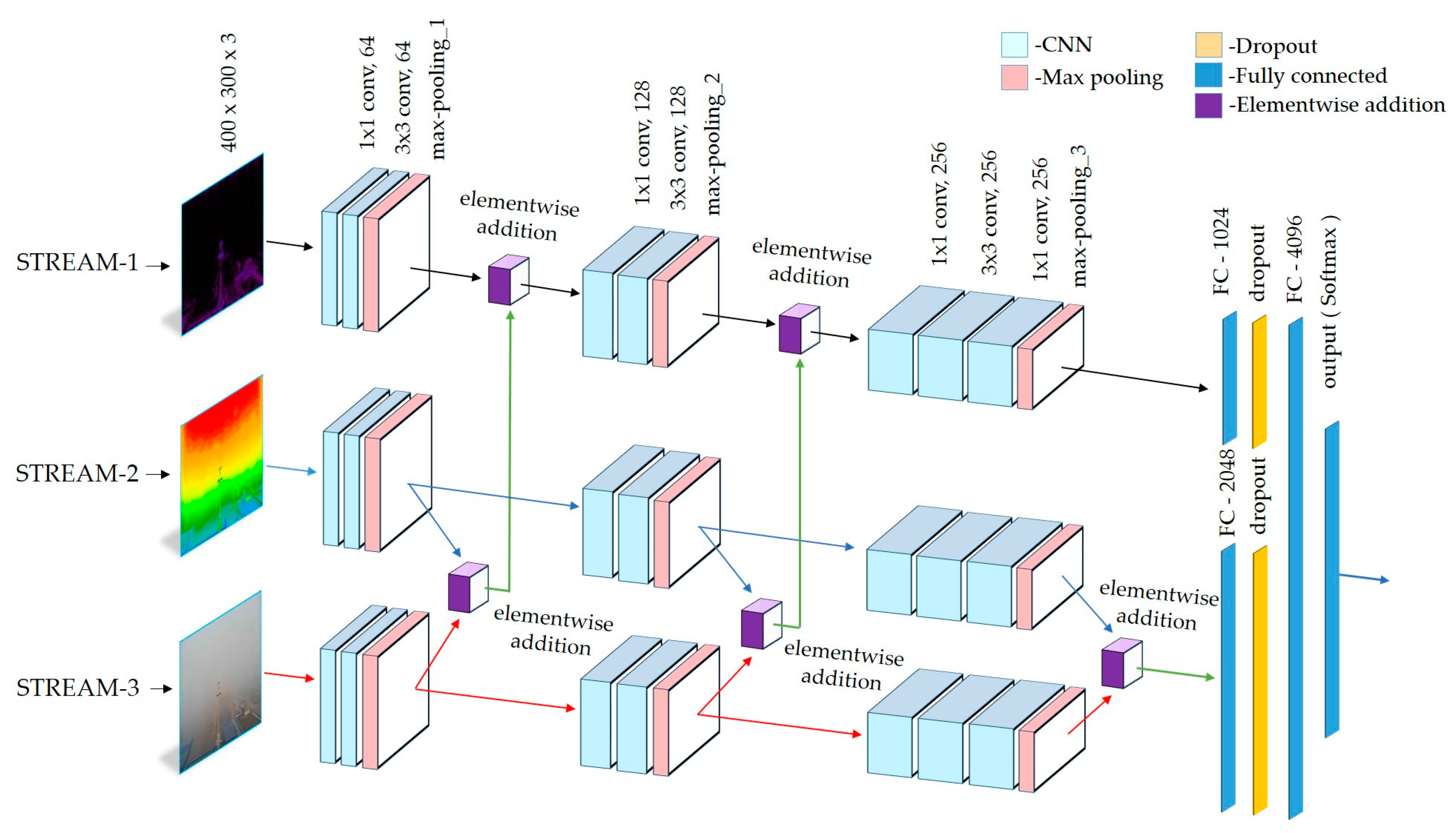
- VisNet: The proposed model based on deep integrated CNN, which receives original (ORG) input images and processes them using spectral and FFT filters prior to training. Instead of utilizing any decision rule, the CNN streams connected fully-connected layers to integrate streams and finally the softmax layer produces outputs.
- VGG-16/FFT + VisNet: The fusion by the weighted sum rule of VGG-16 [66] and VisNet. The purposed model received original images, the VGG-16 was trained with FFT filtered images.
- VGG-16/ORG + VGG-16/SPC + VGG-16/FFT + VisNet: Weighted sum rule utilized to fuse VGG-16 [66] and VisNet. Three VGG-16 [66] were trained with the same parameters, the only difference was the types of input images, VGG-16 was trained with original, spectral filtered, and FFT filtered images (ORG, SPC, and FFT for each VGG-16). VisNet received original images and processed images before training.
5. Conclusions
Author Contributions
Funding
Conflicts of Interest
Appendix A

References
- Guide to Meteorological Instruments and Methods of Observation; World Meteorological Organization: Geneva, Switzerland, 2014; Available online: https://www.wmo.int/pages/prog/www/IMOP/CIMO-Guide.html (accessed on 10 September 2018).
- The International Commission on Illumination—CIE. Termlist. Available online: http://www.cie.co.at/eilv/772 (accessed on 25 September 2018).
- American Meteorological Society. VISIBILITY. Bull. Am. Meteorol. Soc. 2018, 2, 75. [Google Scholar] [CrossRef]
- Dustin, F.; Richard, D. Application of Artificial Neural Network Forecasts to Predict Fog at Canberra International Airport. Available online: https://doi.org/10.1175/WAF980.1 (accessed on 6 December 2018).
- Narasimhan, S.G.; Nayar, S.K. Contrast restoration of weather degraded images. IEEE Trans. Pattern Anal. Mach. Intell. 2003, 25, 713–724. [Google Scholar] [CrossRef]
- Tan, R.T. Visibility in bad weather from a single image. In Proceedings of the IEEE Conference on Computer Vision and Pattern Recognition (CVPR), Anchorage, AK, USA, 23–28 June 2008. [Google Scholar]
- National Highway Traffic Safety Administration. US Department of Transportation. Available online: https://www.nhtsa.gov/ (accessed on 21 September 2018).
- Bruce, H.; Brian, T.; Lindsay, A.; Jurek, G. Hidden Highways: Fog and Traffic Crashes on America’s Roads; AAA Foundation for Traffic Safety: Washington, DC, USA, 2014. [Google Scholar]
- Road Traffic Injuries. World Health Organization, 2018. Available online: https://www.who.int/news-room/fact-sheets/detail/road-traffic-injuries (accessed on 5 January 2019).
- Jon, E. Fog: Deadlier Driving Danger than You Think. Weather Explainers. Available online: https://weather.com/news/news/fog-driving-travel-danger-20121127 (accessed on 8 December 2018).
- Sebastian, J.D.; Philipp, K.; Georg, J.M.; Achim, Z. Forecasting Low-Visibility Procedure States with Tree-Based Statistical Methods; Working Papers in Economics and Statistics; Faculty of Economics and Statistics, University of Innsbruck: Innsbruck, Austria, 2017. [Google Scholar]
- Li, S.; Fu, H.; Lo, W.-L. Meteorological Visibility Evaluation on Webcam Weather Image Using Deep Learning Features. Int. J. Comput. Theory Eng. 20017, 9, 455–461. [Google Scholar] [CrossRef]
- Saulo, B.C.; Frede de, O.C.; Ricardo, F.C.; Antonio, M.V. Fog forecast for the international airport of maceio, brazil using artificial neural network. In Proceedings of the 8th ICSHMO, Foz do Iguaçu, Brazil, 24–28 April 2006; pp. 1741–1750. [Google Scholar]
- Manoel, V.d.A.; Gutemberg, B.F. Neural Network Techniques for Nowcasting of Fog at Guarulhos Airport. Applied Meteorology Laboratory. Available online: www.lma.ufrj.br (accessed on 10 November 2018).
- Philipp, K.; Sebastian, J.D.; Georg, J.M.; Achim, Z. Probabilistic Nowcasting of Low-Visibility Procedure States at Vienna International Airport during Cold Season; Working Papers in Economics and Statistics; University of Innsbruck: Innsbruck, Austria, 2017. [Google Scholar]
- Lei, Z.; Guodong, Z.; Lei, H.; Nan, W. The Application of Deep Learning in Airport Visibility Forecast. Atmos. Clim. Sci. 2017, 7, 314–322. [Google Scholar]
- Rosangela, O.C.; Antonio, L.F.; Francisco, A.S.V.; Adriano, R.B.T. Application of Artificial Neural Networks for Fog Forecast. J. Aerosp. Technol. Manag. 2015, 7, 240–246. [Google Scholar]
- Raouf, B.; Nicolas, H.; Eric, D.; Roland, B.; Nicolas, P. A Model-Driven Approach to Estimate Atmospheric Visibility with Ordinary Cameras. Atmos. Environ. 2011, 45, 5316–5324. [Google Scholar]
- Christos, S.; Dengxin, D.; Luc, V.G. Semantic Foggy Scene Understanding with Synthetic Data. In Proceedings of the Computer Vision and Pattern Recognition (CVPR), Honolulu, HI, USA, 22–25 July 2017. [Google Scholar]
- Olga, S.; James, G.K.; Peter, C.C. A Neural Network Approach to Cloud Detection in AVHRR Images. In Proceedings of the IJCNN-91-Seattle International Joint Conference on Neural Networks, Seattle, WA, USA, 8–12 July 1991. [Google Scholar]
- Palmer, A.H. Visibility. Bulletin of the American Meteorological Society. Available online: https://www.jstor.org/stable/26261872 (accessed on 17 June 2018).
- Chu, W.-T.; Zheng, X.-Y.; Ding, D.-S. Camera as Weather Sensor: Estimating Weather Information from Single Images. J. Vis. Commun. Image Represent. 2017, 46, 233–249. [Google Scholar] [CrossRef]
- Taek, M.K. Atmospheric Visibility Measurements Using Video Cameras: Relative Visibility; National Technical Information Services: Springfield, VA, USA, 2004. [Google Scholar]
- Pomerleau, D. Visibility estimation from a moving vehicle using the RALPH vision system. In Proceedings of the Conference on Intelligent Transportation Systems, Boston, MA, USA, 12–12 November 1997. [Google Scholar]
- Robert, G.H.; Michael, P.M. An Automated Visibility Detection Algorithm Utilizing Camera Imagery. In Proceedings of the 23rd Conference on IIPS, San Antonio, TX, USA, 15 January 2007. [Google Scholar]
- James, V. Surveillance Society: New High-Tech Cameras Are Watching You. Available online: https://www.popularmechanics.com/military/a2398/4236865/ (accessed on 19 November 2018).
- How Many CCTV Cameras in London? Caught on Camera. Available online: https://www.caughtoncamera.net/news/how-many-cctv-cameras-in-london/ (accessed on 25 June 2018).
- Number of CCTV Cameras in South Korea 2013–2017. The Statistics Portal. Available online: https://www.statista.com/statistics/651509/south-korea-cctv-cameras/ (accessed on 2 December 2018).
- Yang, Y.; Cewu, L.; Weiming, W.; Chi-Keung, T. Relative CNN-RNN: Learning Relative Atmospheric Visibility from Images. IEEE Trans. Image Process. 2019, 28, 45–55. [Google Scholar]
- Usman, A.; Olaore, K.O.; Ismaila, G.S. Estimating Visibility Using Some Meteorological Data at Sokoto, Nigeria. Int. J. Basic Appl. Sci. 2013, 01, 810–815. [Google Scholar]
- Vladimir, B.; Ondrej, F.; Lubos, R. Development of system for measuring visibility along the free space optical link using digital camera. In Proceedings of the 24th International Conference Radioelektronika, Bratislava, Slovakia, 15–16 April 2014. [Google Scholar]
- John, D.B.; Mark, S.R. Impacts of Fog Characteristics, Forward Illumination, and Warning Beacon Intensity Distribution on Roadway Hazard Visibility. Sci. World J. 2016, 2016, 4687816. [Google Scholar]
- Nicolas, H.; Jean-Philippe, T.; Jean, L.; Didier, A. Automatic fog detection and estimation of visibility distance through use of an onboard camera. Machine Vision and Applications. Mach. Vision Appl. 2006, 17, 8–20. [Google Scholar]
- Chengwei, L.; Peng, P. Visibility measurement using multi-angle forward scattering by liquid droplets. Meas. Sci. Technol. 2012, 23, 105802. [Google Scholar]
- Nicolas, H.; Didier, A.; Eric, D.; Jean-Philippe, T. Experimental Validation of Dedicated Methods to In-Vehicle Estimation of Atmospheric Visibility Distance. IEEE Trans. Instrum. Meas. 2008, 57, 2218–2225. [Google Scholar]
- Cheng, X.; Liu, G.; Hedman, A.; Wang, K.; Li, H. Expressway visibility estimation based on image entropy and piecewise stationary time series analysis. In Proceedings of the CVPR, Boston, MA, USA, 8–10 June 2015. [Google Scholar]
- Kipfer, K. Fog Prediction with Deep Neural Networks; ETH Zurich: Zurich, Switzerland, 2017. [Google Scholar]
- Nicolas, H.; Raphael, L.; Didier, A. Estimation of the Visibility Distance by Stereovision: A Generic Approach. IEICE Trans. Inf. Syst. 2005, E89-D, 590–593. [Google Scholar]
- Viola, C.; Michele, C.; Jocelyne, D. Distance Perception of Vehicle Rear Lights in Fog. Hum. Factors 2001, 43, 442–451. [Google Scholar]
- Jeevan, S.; Usha, L. Estimation of visibility distance in images under foggy weather condition. Int. J. Adv. Comput. Electron. Technol. 2016, 3, 11–16. [Google Scholar]
- Ginneken, B.; Setio, A.; Jacobs, C.; Ciompi, F. Off-the-shelf convolutional neural network features for pulmonary nodule detection in computed tomography scans. In Proceedings of the IEEE 12th International Symposium on Biomedical Imaging (ISBI), New York, NY, USA, 16–19 April 2015; pp. 286–289. [Google Scholar]
- LeCun, Y.; Bottou, L.; Bengio, Y.; Haffner, P. Gradient-based learning applied to document recognition. Proc. IEEE 1998, 86, 2278–2324. [Google Scholar] [CrossRef]
- Carneiro, G.; Nascimento, J. Combining multiple dynamic models and deep learning architectures for tracking the left ventricle endocardium in ultrasound data. IEEE Trans. Pattern Anal. Mach. Intell. 2013, 35, 2592–2607. [Google Scholar] [CrossRef]
- Schleg, T.; Ofiner, J.; Langs, G. Unsupervised pre-training across image domains improves lung tissue classification. In Medical Computer Vision: Algorithms for Big Data; Springer: New York, NY, USA, 2014; pp. 82–93. [Google Scholar]
- Shin, H. Interleaved text/image deep mining on a large-scale radiology image database. In Proceedings of the IEEE Conference (CVPR), Boston, MA, USA, 8–10 June 2015; pp. 1090–1099. [Google Scholar]
- Russakovsky, O. ImageNet large scale visual recognition challenge. Int. J. Comput. Vison 2015, 115, 211–252. [Google Scholar] [CrossRef]
- Mohammad, R.; Masoud, M.; Yun, Z.; Bahram, S. Deep Convolutional Neural Network for Complex Wetland Classification Using Optical Remote Sensing Imagery. IEEE J. Sel. Top. Appl. Earth Obs. Remote Sens. 2018, 11, 3030–3039. [Google Scholar]
- Shao, Z.; Cai, J. Remote Sensing Image Fusion with Deep Convolutional Neural Network. IEEE J. Sel. Top. Appl. Earth Obs. Remote Sens. 2018, 11, 1656–1669. [Google Scholar] [CrossRef]
- Brucoli, M.; Leonarda, C.; Grassi, G. Implementation of cellular neural networks for heteroassociative and autoassociative memories. In Proceedings of the Cellular Neural Networks and their Applications (CNNA-96), Seville, Spain, 24–26 June 1996. [Google Scholar]
- Shalygo, Y. Phenomenology of Tensor Modulation in Elementary Kinetic Automata. Complex Syst. 2016, 25, 195–221. [Google Scholar] [CrossRef]
- Shin, H.C.; Roth, H.R.; Gao, M.; Lu, L.; Xu, Z.; Nogues, I.; Yao, J.; Mollura, D.; Summers, R.M. Deep Convolutional Neural Networks for Computer-Aided Detection: CNN Architectures. Dataset Characteristics and Transfer Learning. IEEE Trans. Med. Imaging 2016, 35, 1285–1298. [Google Scholar] [CrossRef]
- Rachid, B.; Dominique, G. Impact of Reduced Visibility from Fog on Traffic Sign Detection. In Proceedings of the IEEE Intelligent Vehicles Symposium (IV), Dearborn, MI, USA, 8–11 June 2014. [Google Scholar]
- Tasadduq, I.; Rehman, S.; Bubshait, K. Application of neural networks for the prediction of hourly mean surface temperature in Saudi Arabia. Renew. Energy 2002, 25, 545–554. [Google Scholar] [CrossRef]
- Gardner, M.W.; Dorling, S.R. Artificial neural networks (the multilayer perceptron)—A review of applications in the atmospheric sciences. Atmos. Environ. 1998, 3, 2627–2636. [Google Scholar] [CrossRef]
- Rummelhart, D.E.; McCelland, J.L. Parallel Distributed Processing; The MIT Press: Cambridge, MA, USA, July 1986; Volume 1, p. 567. [Google Scholar]
- Marzban, C. The ROC curve and the area under it as a performance measure. Weather Forecast. 2004, 19, 1106–1114. [Google Scholar] [CrossRef]
- Stumpf, G.J. A neural network for tornado prediction based on Doppler radar–derived attributes. J. Appl. Meteor. 1996, 35, 617–626. [Google Scholar]
- Hall, T.; Brooks, H.E.; Doswel, C.A. Precipitation forecasting using a neural network. Weather Forecast. 1999, 14, 338–345. [Google Scholar] [CrossRef]
- Kwon, T.M. An Automatic Visibility Measurement System Based on Video Cameras. Ph.D. Thesis, Final Report. Department of Electrical Engineering, University of Minnesota, Duluth, MN, USA, 1998. [Google Scholar]
- Pasini, A.; Potest, S. Short-Range Visibility Forecast by Means of Neural-Network Modelling: A Case-Study. J. Nuovo Cimento - Societa Italiana di Fisica Sezione 1995, 18, 505–516. [Google Scholar] [CrossRef]
- Gabriel, L.; Juan, L.; Inmaculada, P.; Christian, A.G. Visibility estimates from atmospheric and radiometric variables using artificial neural networks. WIT Trans. Ecol. Environ. 2017, 211, 129–136. [Google Scholar]
- Kai, W.; Hong, Z.; Aixia, L.; Zhipeng, B. The Risk Neural Network Based Visibility Forecast. In Proceedings of the Fifth International Conference on Natural Computation IEEE, Tianjin, China, 14–16 August 2009. [Google Scholar]
- Hazar, C.; Faouzi, K.; Hichem, B.; Fatma, O.; Ansar-Ul-Haque, Y. A Neural network approach to visibility range estimation under foggy weather conditions. Procedia Comput. Sci. 2017, 113, 466–471. [Google Scholar]
- Alex, K.; Ilya, S.; Geoffrey, E.H. ImageNet Classification with Deep Convolutional Neural Networks. In Advances in Neural Information Processing Systems 25; Curran Associates, Inc.: New York, NY, USA, 2012; pp. 1097–1105. [Google Scholar]
- He, K.; Zhang, X.; Ren, S.; Sun, J. Deep Residual Learning for Image Recognition. In Proceedings of the Computer Vision and Pattern Recognition (CVPR), Boston, MA, USA, 8–10 June 2015. [Google Scholar]
- Karen, S.; Andrew, Z. Very Deep Convolutional Networks for Large-Scale Image Recognition. In Proceedings of the Computer Vision and Pattern Recognition (CVPR), Columbus, OH, USA, 23–28 June 2014. [Google Scholar]
- Joanne, P.; Kuk, L.; Gary, M. An Introduction to Logistic Regression Analysis and Reporting. J. Educ. Res. 2002, 96, 3–14. [Google Scholar]
- Marti, A. Support Vector Machines. IEEE Intell. Syst. Appl. 1998, 13, 18–28. [Google Scholar]
- Jung, H.; Lee, R.; Lee, S.; Hwang, W. Residual Convolutional Neural Network Revisited with Active Weighted Mapping. Computer Vision and Pattern Recognition. Available online: https://arxiv.org/abs/1811.06878 (accessed on 27 December 2018).
- He, K.; Zhang, X.; Ren, S.; Sun, J. Identity Mappings in Deep Residual Networks. In European Conference on Computer Vision; Springer: Berlin/Heidelberg, Germany, 2016; pp. 630–645. [Google Scholar]
- He, K.; Zhang, X.; Ren, S.; Sun, J. Deep Residual Learning for Image Recognition. In Proceedings of the IEEE conference on Computer Vision and Pattern Recognition (CVPR), Las Vegas, NV, USA, 27–30 June 2016; Volume 1, pp. 770–778. [Google Scholar] [CrossRef]
- ImageNet-Large Scale Visual Recognition Challenge 2014 (ILSVRC2014). Available online: http://image-net.org/challenges/LSVRC/2014/index (accessed on 14 June 2018).
- Caren, M.; Stephen, L.; Brad, C. Ceiling and Visibility Forecasts via Neural Networks. Weather Forecast. 2007, 22, 466–479. [Google Scholar]
- Robert, H.; Michael, M.; David, C. Video System for Monitoring and Reporting Weather Conditions. U.S. Patent Application #US20020181739A1; MIT, 5 December 2002. Available online: https://patents.google.com/patent/US20020181739 (accessed on 10 October 2018).
- Robert, G.; Hallowell, P.; Michael, P.; Matthews, P.; Pisano, A. Automated Extraction of Weather Variables from Camera Imagery. In Proceedings of the 2005 Mid-Continent Transportation Research Symposium, Ames, Iowa, 18–19 August 2005. [Google Scholar]
- Rajib, P.; Heekwan, L. Algorithm Development of a Visibility Monitoring Technique Using Digital Image Analysis. Asian J. Atmos. Environ. 2011, 5, 8–20. [Google Scholar]
- An, M.; Guo, Z.; Li, J.; Zhou, T. Visibility Detection Based on Traffic Camera Imagery. In Proceedings of the 3rd International Conference on Information Sciences and Interaction Sciences, Chengdu, China, 23–25 June 2010. [Google Scholar]
- Roberto, C.; Peter, F.; Christian, R.; Christiaan, C.S.; Jakub, T.; Arthur, V. Fog detection from camera images. In Proceedings of the SWI Proceedings, Nijmegen, The Netherlands, 25–29 January 2016. [Google Scholar]
- Fan, G.; Hui, P.; Jin, T.; Beiji, Z.; Chenggong, T. Visibility detection approach to road scene foggy images. KSII Trans. Internet Inf. Syst. 2016, 10, 9. [Google Scholar]
- Tarel, J.-P.; Bremond, R.; Dumont, E.; Joulan, K. Comparison between optical and computer vision estimates of visibility in daytime fog. In Proceedings of the 28th CIE Session, Manchester, UK, 28 June–4 July 2015. [Google Scholar]
- Xiang, W.; Xiao, J.; Wang, C.; Liu, Y. A New Model for Daytime Visibility Index Estimation Fused Average Sobel Gradient and Dark Channel Ratio. In Proceedings of the 3rd International Conference on Computer Science and Network Technology, Dalian, China, 12–13 October 2013. [Google Scholar]
- Li, Y. Comprehensive Visibility Indicator Algorithm for Adaptable Speed Limit Control in Intelligent Transportation Systems; A Presented Work to the University of Guelph; University of Guelph: Guelph, ON, Canada, 2018. [Google Scholar]
- Sriparna, B.; Sangita, R.; Chaudhuri, S.S. Effect of patch size and haziness factor on visibility using DCP. In Proceedings of the 2nd International Conference for Convergence in Technology (I2CT), Mumbai, India, 7–9 April 2017. [Google Scholar]
- Hou, Z.; Yau, W. Visible entropy: A measure for image visibility. In Proceedings of the International Conference on Pattern Recognition, Istanbul, Turkey, 23–26 August 2010. [Google Scholar]
- Wiel, W.; Martin, R. Exploration of fog detection and visibility estimation from camera images. In Proceedings of the TECO, Madrid, Spain, 27–30 September 2016. [Google Scholar]
- Miclea, R.C.; Silea, I. Visibility detection in foggy environment. In Proceedings of the International Conference on Control Systems and Computer Science, Bucharest, Romania, 27–29 May 2015. [Google Scholar]
- Tarel, J.P.; Hautiere, N.; Cord, A.; Gruyer, D.; Halmaoui, H. Improved visibility of road scene images under heterogeneous fog. In Proceedings of the IEEE Intelligent Vehicles Symposium, San Diego, CA, USA, 21–24 June 2010; pp. 478–485. [Google Scholar]
- Gallen, R.; Cord, A.; Hautiere, N.; Dumont, E.; Aubert, D. Nighttime visibility analysis and estimation method in the presence of dense fog. IEEE Trans. Intell. Transp. Syst. 2015, 16, 310–320. [Google Scholar] [CrossRef]
- Clement, B.; Nicolas, H.; Brigitte, A. Vehicle Dynamics Estimation for Camera-based Visibility Distance Estimation. In Proceedings of the IEEE/RSJ International Conference on Intelligent Robots and Systems, Nice, France, 22–26 September 2008. [Google Scholar]
- Clement, B.; Nicolas, H.; Brigitte, A. Visibility distance estimation based on structure from motion. In Proceedings of the 11th International Conference on Control Automation Robotics and Vision, Singapore, 7–10 December 2011. [Google Scholar]
- Gallen, R.; Cord, A.; Hautiere, N.; Aubert, D. Towards night fog detection through use of in-vehicle multipurpose cameras. In Proceedings of the IEEE Intelligent Vehicles Symposium (IV), Baden-Baden, Germany, 5–9 June 2011. [Google Scholar]
- Colomb, M.; Hirech, K.; Andre, P.; Boreux, J.; Lacote, P.; Dufour, J. An innovative artificial fog production device improved in the European project “FOG”. Atmos. Res. 2008, 87, 242–251. [Google Scholar] [CrossRef]
- Lee, S.; Yun, S.; Nam, Ju.; Won, C.S.; Jung, S. A review on dark channel prior based image dehazing algorithms. URASIP J. Image Video Process. 2016, 2016. [Google Scholar] [CrossRef]
- Boyi, L.; Wenqi, R.; Dengpan, F.; Dacheng, T.; Dan, F.; Wenjun, Z.; Zhangyang, W. Benchmarking Single-Image Dehazing and Beyond. IEEE Trans. Image Process. 2019, 28, 492–505. [Google Scholar]
- Pranjal, G.; Shailender, G.; Bharat, B.; Prem, C.V. A Hybrid Defogging Technique based on Anisotropic Diffusion and IDCP using Guided Filter. Int. J. Signal Process. Image Process. Pattern Recognit. 2015, 8, 123–140. [Google Scholar]
- Yeejin, L.; Keigo, H.; Truong, Q.N. Joint Defogging and Demosaicking. IEEE Trans. Image Process. 2017, 26, 3051–3063. [Google Scholar]
- William, H.P.; Saul, A.T.; William, T.V.; Brian, P.F. Numerical recipes. In the Art of Scientific Computing. Available online: https://www.cambridge.org/9780521880688 (accessed on 18 June 2018).
- Yong, H.L.; Jeong-Soon, L.; Seon, K.P.; Dong-Eon, Ch.; Hee-Sang, L. Temporal and spatial characteristics of fog occurrence over the Korean Peninsula. J. Geophys. Res. 2010, 115, D14117. [Google Scholar]
- Anitha, T.G.; Ramachandran, S. Novel Algorithms for 2-D FFT and its Inverse for Image Compression. In Proceedings of the IEEE International Conference on Signal Processing, Image Processing and Pattern Recognition [ICSIPRl], Coimbatore, India, 7–8 February 2013. [Google Scholar]
- Faisal, M.; Mart, T.; Lars-Goran, O.; Ulf, S. 2D Discrete Fourier Transform with Simultaneous Edge Artifact Removal for Real-Time Applications. In Proceedings of the 2015 International Conference on Field Programmable Technology (FPT), Queenstown, New Zealand, 7–9 December 2016. [Google Scholar]
- Fisher, R.; Perkins, S.; Walker, A.; Wolfart, E. Fourier Transform. Available online: https://homepages.inf.ed.ac.uk/rbf/HIPR2/fourier.htm (accessed on 27 July 2018).
- Paul, B. Discrete Fourier Transform and Fast Fourier Transform. Available online: http://paulbourke.net/miscellaneous/dft/ (accessed on 19 August 2018).
- James, W.; Cooley, W.; John, W.T. An Algorithm for the Machine Calculation of Complex Fourier series. Math. Comput. Am. Math. Soc. 1965, 19, 297–301. [Google Scholar]
- Tutatchikov, V.S.; Kiselev, O.I.; Mikhail, N. Calculating the n-dimensional fast Fourier transform. Pattern Recognit. Image Anal. 2013, 23, 429–433. [Google Scholar] [CrossRef]
- Vaclav, H. Fourier transform, in 1D and in 2D., keynote at Czech Institute of Informatics, Robotics and Cybernetics. Available online: http://people.ciirc.cvut.cz/hlavac (accessed on 1 December 2018).
- Nabeel, S.; Peter, A.M.; Lynn, A. Implementation of a 2-D Fast Fourier Transform on a FPGA-Based Custom Computing Machine. In Proceedings of the International Workshop on Field Programmable Logic and Applications, Field-Programmable Logic and Applications, Oxford, UK, 29 August–1 September 1995; Springer: Berlin/Heidelberg, Germany, 1995; pp. 282–290. [Google Scholar]
- Jang, J.H.; Ra, J.B. Pseudo-Color Image Fusion Based on Intensity-Hue-Saturation Color Space. In Proceedings of the IEEE International Conference on Multisensor Fusion and Integration for Intelligent Systems, Seoul, Korea, 20–22 August 2008. [Google Scholar]
- Adrian, F.; Alan, R. Colour Space Conversions. Available online: https://poynton.ca/PDFs/coloureq.pdf (accessed on 11 October 2018).
- Khosravi, M.R.; Rostami, H.; Ahmadi, G.R.; Mansouri, S.; Keshavarz, A. A New Pseudo-color Technique Based on Intensity Information Protection for Passive Sensor Imagery. Int. J. Electron. Commun. Comput. Eng. 2015, 6, 324–329. [Google Scholar]
- Kenneth, M. Why We Use Bad Color Maps and What You Can Do About It? Electron. Imaging 2016, 16, 1–6. [Google Scholar]
- Scott, L. Severe Weather in the Pacific Northwest. Cooperative Institute for Meteorological Satellite Studies (CIMSS), University of Wisconsin: Madison, WI, USA, 15 October 2016. Available online: http://cimss.ssec.wisc.edu/goes/blog/archives/22329 (accessed on 15 January 2019).
- Peter, K. Good Colour Maps: How to Design Them. Available online: http://arxiv.org/abs/1509.03700 (accessed on 23 September 2018).
- Michael, B.; Robert, H. Rendering Planar Cuts Through Quadratic and Cubic Finite Elements. In Proceedings of the IEEE Visualization, Austin, TX, USA, 10–15 October 2004. [Google Scholar]
- Colin, W. Information Visualization: Perception for Design. In Morgan Kaufmann, 2nd ed.; Elsevier: Amsterdam, The Netherlands, 2004. [Google Scholar]
- Rene, B.; Fons, R. The Rainbow Color Map, ROOT data Analysis Framework. Available online: https://root.cern.ch/rainbow-color-map (accessed on 03 January 2019).
- CS231n. Convolutional Neural Networks for Visual Recognition. Available online: http://cs231n.github.io/convolutional-networks/#overview (accessed on 23 February 2017).
- Nair, V.; Hinton, G.E. Rectified linear units improve restricted Boltzmann machines. In Proceedings of the 27th International Conference on Machine Learning, Haifa, Israel, 21–24 June 2010; pp. 807–814. [Google Scholar]
- Srivastava, N.; Hinton, G.; Krizhevsky, A.; Sutskever, I.; Salakhutdinov, R. Dropout: A simple way to prevent neural networks from overfitting. J. Mach. Learn. Res. 2014, 15, 1929–1958. [Google Scholar]
- Jong, H.K.; Hyung, G.H.; Kang, R.P. Convolutional Neural Network-Based Human Detection in Nighttime Images Using Visible Light Camera Sensors. J. Sens. 2017, 17, 1065. [Google Scholar] [CrossRef]
- Kingma, D.P.; Ba, J. Adam: A method for stochastic optimization. In Proceedings of the International Conference for Learning Representations (ICLR), San Diego, CA, USA, 7–9 May 2015; pp. 1–15. [Google Scholar]


| Category | Used Methods | Evaluation Range [m] | Advantages | Disadvantages |
|---|---|---|---|---|
| ANN-based methods | Uses feed-forward neural networks [63] and FROSI dataset [52] | 60–250 | High evaluation accuracy on the FROSI dataset; Fast evaluation speed; | Classifies only synthetic images and cannot be used for real-world images; Only short visibility range can be estimated; |
| Combination of CNN and RNN are used for learning atmospheric visibility [29]. Relative SVM [29] is used on top of CNN-RNN model. Input images collected from the Internet. | 300–800 | Can effectively adapt to both small and big data scenario; | Computationally costly and consumes long time to train; Uses manual annotations instead of more reliable sensors; | |
| Pre-trained CNN model (AlexNet [12]) is used to classify webcam weather images [12]. | 5000–35,000 | Can evaluate a dataset of images with smaller resolutions; Faster training because of using cropped patches of input images; | Uses an unbalanced dataset; Test accuracy is very low (61.8%); Reveals too high prediction error (±3 km); Reference objects are required for accurate classification; | |
| Deep neural networks for visibility forecasting [16]. Uses 24 h a day observation data from 2007 to 2016 (these inputs are temperature, dew point temperature, relative humidity, wind direction, and wind speed.) | 0–5000 | A working application for aviation meteorological services at the airport; | Achieves a big absolute error (the absolute error of hourly visibility is 706 m. The absolute error is 325 m when visibility ≤1000 m); Several types of input data are required that collected using expensive sensors; | |
| Visibility distance is evaluated using a system consists of three layers of forward-transfer, back-propagation, and risk neural network [62]. A meteorological dataset, which collected within 5 years, utilized to verify the model. | 0–10,000 | A higher risk is given to low-visibility and vice-versa; Outperforms standard neural networks and baseline regression models; | Needs a collection of several daily data that require high-cost measurements to predict future hours; Uses only the average values, not real values, of the data; Focuses mostly on low-visibility; Evaluation of high visibility conditions is error-prone; Carefully parameter adjusting is required to avoid biased learning process; | |
| Statistical methods | Estimation of atmospheric visibility distance via ordinary outdoor cameras based on the contrast expectation in the scene [18]. | 1–5000 | Uses publicly available dataset; No need to calibrate the system to evaluate visibility; | Model-driven; More effective for high-visibility; An estimation low-visibility is error-prone; Requires extra meteorological sensors to obtain important values; |
| A model based on the Sobel edge detection algorithm and normalized edge extraction method to detect visibility from camera imagery [25]. | 400–16,000 | Uses small amounts of images; Automatic and fast computation; | Cannot predict the distance if visibility is less than 400 m; Uses high-cost camera (COHU 3960 Series environmental camera); | |
| Uses Gaussian image entropy and piecewise stationary time series analysis algorithms [36]. A region of interest is extracted taking into account the relative ratios of image entropy to improve performance. | 0–600 | Uses a very big dataset (2,016,000 frames) to verify the model; | Can be used only road scenes; Works effectively only in uniform fog; | |
| Exploration of visibility estimation from camera imagery [85]. Methods are landmark discrimination using edge detection, contrast reduction between targets, global image features (mean edge, transmission estimation using DCP), decision tree, and regression methods. | 250–5000 | Uses low-cost cameras; No need camera calibration; Low-resolution images can be evaluated; | Target objects are needed; Different methods require different reference points as targets; Can be used in a fixed camera environment; |
| Dataset | Range | Total Number of Selected Images | Visibility Distance [m] | Number of Classes | Range Between Classes [m] |
|---|---|---|---|---|---|
| FOVI | Long-range | 140,000 | 0 to 20,000 | 41 | 500 |
| Short-range | 100,000 | 0 to 1000 | 21 | 50 | |
| FROSI | Short-range | 3528 | 0 to >250 | 7 | 50 |
| STREAM-1 | STREAM-2 | STREAM-3 | ||||||
|---|---|---|---|---|---|---|---|---|
| Layer Type | Num. of Filters | Size of Feature Map | Num. of Filters | Size of Feature Map | Num. of Filters | Size of Feature Map | Size of Kernel | Num. of Stride |
| Image input layer (weight × height × channel) | 400 × 300 × 3 | 400 × 300 × 3 | 400 × 300 × 3 | |||||
| 1th convolutional layer | 64 | 400 × 300 × 64 | 64 | 400 × 300 × 64 | 64 | 400 × 300 × 64 | 1 × 1 × 3 | 1 × 1 |
| 2nd convolutional layer | 64 | 398 × 298 × 64 | 64 | 398 × 298 × 64 | 64 | 398 × 298 × 64 | 3 × 3 × 3 | 1 × 1 |
| Max-pooling layer | 1 | 199 × 149 × 64 | 1 | 199 × 149 × 64 | 1 | 199 × 149 × 64 | 2 × 2 | 2 × 2 |
| Elementwise addition | ||||||||
| Elementwise addition | ||||||||
| 3rd convolutional layer | 128 | 199 × 149 × 128 | 128 | 199 × 149 × 128 | 128 | 199 × 149 × 128 | 1 × 1 × 3 | 1 × 1 |
| 4th convolutional layer | 128 | 197 × 147 × 128 | 128 | 197 × 147 × 128 | 128 | 197 × 147 × 128 | 3 × 3 × 3 | 1 × 1 |
| Max-pooling layer | 1 | 98 × 73 × 128 | 1 | 98 × 73 × 128 | 1 | 98 × 73 × 128 | 2 × 2 | 2 × 2 |
| Elementwise addition | ||||||||
| Elementwise addition | ||||||||
| 5th convolutional layer | 256 | 98 × 73 × 256 | 256 | 98 × 73 × 256 | 256 | 98 × 73 × 256 | 1 × 1 × 3 | 1 × 1 |
| 6nd convolutional layer | 256 | 48 × 36 × 256 | 256 | 48 × 36 × 256 | 256 | 48 × 36 × 256 | 3 × 3 × 3 | 2 × 2 |
| 7nd convolutional layer | 256 | 48 × 36 × 256 | 256 | 48 × 36 × 256 | 256 | 48 × 36 × 256 | 1 × 1 × 3 | 1 × 1 |
| Max-pooling layer | 1 | 24 × 18 × 256 | 1 | 24 × 18 × 256 | 1 | 24 × 18 × 256 | 2 × 2 | 2 × 2 |
| Elementwise addition | ||||||||
| 1st and 2nd fully connected layers | 1024 | 2048 | ||||||
| Dropout layers | 1024 | 2048 | ||||||
| 3rd fully connected layer | 4096 | |||||||
| Classification layer (output layer) | 41 or 21 or 7 | |||||||
| Item | Content |
|---|---|
| CPU | AMD Ryzen Threadripper 1950X 16-Core Processor |
| GPU | NVIDIA GeForce GTX 1080 Ti |
| RAM | 64 GB |
| Operating system | Windows 10 |
| Programming language | Python 3.6 |
| Deep learning library | Tensorflow 1.11 |
| Cuda | cuda 9.2 |
| Dataset | Range | Validation Accuracy | Test Accuracy |
|---|---|---|---|
| FOVI | Long-range | 93.04 | 91.30 |
| Short-range | 91.77 | 89.51 | |
| FROSI | Short-range | 96.80 | 94.03 |
| Models | FOVI Dataset (Long-Range) | FOVI Dataset (Short-Range) | FROSI Dataset (Short-Range) | |||
|---|---|---|---|---|---|---|
| Val. Acc. | Test Acc. | Val. Acc. | Test Acc. | Val. Acc. | Test Acc. | |
| Simple neural network [63] | 48.0 | 45.2 | 42.9 | 38.1 | 58.8 | 57.0 |
| Relative SVM [29] | 69.7 | 68.5 | 59.0 | 57.0 | 73.0 | 72.2 |
| Relative CNN-RNN [29] | 82.2 | 81.3 | 79.0 | 78.4 | 85.5 | 84.4 |
| ResNet-50 [65] | 72.0 | 70.9 | 71.8 | 68.6 | 82.1 | 79.2 |
| VGG-16 [66] | 89.6 | 89.0 | 89.0 | 88.5 | 88.6 | 91.0 |
| Alex-Net [12] | 87.3 | 86.4 | 83.4 | 81.0 | 88.3 | 88.7 |
| VisNet | 93.4 | 91.3 | 90.8 | 89.5 | 96.8 | 94.0 |
| Models | FOVI Dataset (Long-Range) | FOVI Dataset (Short-Range) | FROSI Dataset (Short-Range) | |||
|---|---|---|---|---|---|---|
| Val. Error | Test Error | Val. Error | Test Error | Val. Error | Test Error | |
| Simple neural network [63] | 19.5 | 15.8 | 18.6 | 17.9 | 12.9 | 11.0 |
| Relative SVM [29] | 14.7 | 13.1 | 16.3 | 14.5 | 13.1 | 11.9 |
| Relative CNN-RNN [29] | 12.4 | 12.2 | 11.2 | 11.7 | 11.8 | 10.7 |
| ResNet-50 [65] | 11.8 | 10.7 | 14.4 | 13.7 | 9.5 | 9.7 |
| VGG-16 [66] | 10.1 | 9.9 | 10.4 | 10.0 | 8.0 | 7.8 |
| Alex-Net [12] | 11.4 | 10.9 | 11.3 | 11.1 | 9.1 | 8.9 |
| VisNet | 9.7 | 9.5 | 9.9 | 9.8 | 7.5 | 7.5 |
| Models | FOVI Dataset (Long-Range) | FOVI Dataset (Short-Range) | FROSI Dataset (Short-Range) | |||||||||
|---|---|---|---|---|---|---|---|---|---|---|---|---|
| ORG | SPC | FFT | Sum. | ORG | SPC | FFT | Sum. | ORG | SPC | FFT | Sum. | |
| Simple neural network [63] | 45.2 | 41.9 | 51.3 | 49.8 | 38.1 | 36.1 | 37.6 | 37.4 | 57.0 | 52.1 | 53.8 | 55.0 |
| Relative SVM [29] | 68.5 | 59.0 | 61.1 | 65.6 | 57.0 | 55.6 | 58.3 | 57.0 | 72.2 | 69.6 | 70.5 | 71.2 |
| Relative CNN-RNN [29] | 81.3 | 77.0 | 75.6 | 78.0 | 78.4 | 71.6 | 75.5 | 76.0 | 84.4 | 73.5 | 79.3 | 79.8 |
| ResNet-50 [65] | 70.9 | 61.9 | 73.4 | 71.2 | 68.6 | 60.0 | 67.5 | 64.8 | 79.2 | 76.7 | 78.0 | 78.1 |
| VGG-16 [66] | 89.0 | 79.7 | 81.0 | 86.7 | 88.5 | 79.8 | 81.1 | 85.2 | 91.0 | 86.4 | 88.2 | 89.3 |
| Alex-Net [12] | 86.4 | 76.0 | 78.5 | 82.1 | 81.0 | 76.3 | 77.1 | 78.2 | 88.7 | 79.0 | 83.6 | 84.7 |
| VisNet (single STREAM) | 70.1 | 70.5 | 79.1 | 74.7 | 72.7 | 69.4 | 71.9 | 71.3 | 78.8 | 75.6 | 80.3 | 78.8 |
| Models | FOVI Dataset (Long-Range) | FOVI Dataset (Short-Range) | FROSI Dataset (Short-Range) |
|---|---|---|---|
| VisNet | 91.3 | 89.5 | 94.0 |
| VGG-16/ORG + VisNet | 91.8 | 90.0 | 94.15 |
| VGG-16/SPC + VisNet | 91.5 | 89.53 | 94.25 |
| VGG-16/FFT + VisNet | 91.3 | 89.8 | 94.4 |
| VGG-16/ORG + VGG-16/SPC + VGG-16/FFT + VisNet | 91.40 | 91.8 | 94.2 |
| Net. Name | Convolutional Layers | Class. Acc. [%] | |||||||
|---|---|---|---|---|---|---|---|---|---|
| C-1 | C-2 | C-3 | C-4 | C-5 | C-6 | C-7 | C-8 | ||
| CNN-1 | 32 * FS 3 × 3 MS 199 × 149 Stride 2 | 64 FS 3 × 3 MS 99 × 74 Stride 2 | 128 FS 3 × 3 MS 49 × 36 Stride 2 | 256 FS 3 × 3 MS 24 × 17 Stride 2 | 512 FS 3 × 3 MS 11 × 8 Stride 2 | – | – | – | 78.3 - 75.4 - 81.1 |
| CNN-2 | 32 FS 3 × 3 MS 199 × 149 Stride 2 | 64 FS 3 × 3 MS 99 × 74 Stride 2 | 128 FS 3 × 3 MS 49 × 36 Stride 2 | 128 FS 1 × 1 MS 49 × 36 Stride 1 | 256 FS 3 × 3 MS 24 × 17 Stride 2 | 256 FS 1 × 1 MS 24 × 17 Stride 1 | – | – | 86.0 - 83.1 - 87.2 |
| CNN-3 | 64 FS 1 × 1 MS 400 × 300 Stride 1 | 64 FS 3 × 3 MS 398 × 298 Stride 1 | 128 FS 1 × 1 MS 199 × 149 Stride 1 | 128 FS 3 × 3 MS 197 × 147 Stride 1 | 256 FS 1×1 MS 98×73 Stride 1 | 256 FS 3 × 3 MS 48 × 36 Stride 2 | 256 FS 1 × 1 MS 48 × 36 Stride 1 | – | 91.3 - 89.5 - 94.0 |
| CNN-4 | 64 FS 1 × 1 MS 400 ×3 00 Stride 1 | 64 FS 3 × 3 MS 199 × 149 Stride 2 | 128 FS 1 × 1 MS 199 × 149 Stride 1 | 128 FS 3 × 3 MS 99 × 74 Stride 2 | 256 FS 1 × 1 MS 99 × 74 Stride 1 | 256 FS 3 × 3 MS 49 × 36 Stride 2 | 512 FS 1 × 1 MS 49 × 36 Stride 1 | 512 FS 3 × 3 MS 24 × 17 Stride 2 | 84.0 - 82.3 - 78.2 |
| CNN-5 | 64 FS 3 × 3 MS 400 × 300 Stride 1 | 128 FS 3 × 3 MS 199 × 149 Stride 2 | 256 FS 1 × 1 MS 199 × 149 Stride 1 | 256 FS 3 × 3 MS 99 × 74 Stride 2 | 256 FS 1 × 1 MS 99 × 74 Stride 1 | 512 FS 1 × 1 MS 99 × 74 Stride 1 | 512 FS 3 × 3 MS 49 × 36 Stride 2 | 512 FS 1 × 1 MS 49 × 36 Stride 1 | 83.0 - 77.1 - 71.7 |
© 2019 by the authors. Licensee MDPI, Basel, Switzerland. This article is an open access article distributed under the terms and conditions of the Creative Commons Attribution (CC BY) license (http://creativecommons.org/licenses/by/4.0/).
Share and Cite
Palvanov, A.; Cho, Y.I. VisNet: Deep Convolutional Neural Networks for Forecasting Atmospheric Visibility. Sensors 2019, 19, 1343. https://doi.org/10.3390/s19061343
Palvanov A, Cho YI. VisNet: Deep Convolutional Neural Networks for Forecasting Atmospheric Visibility. Sensors. 2019; 19(6):1343. https://doi.org/10.3390/s19061343
Chicago/Turabian StylePalvanov, Akmaljon, and Young Im Cho. 2019. "VisNet: Deep Convolutional Neural Networks for Forecasting Atmospheric Visibility" Sensors 19, no. 6: 1343. https://doi.org/10.3390/s19061343
APA StylePalvanov, A., & Cho, Y. I. (2019). VisNet: Deep Convolutional Neural Networks for Forecasting Atmospheric Visibility. Sensors, 19(6), 1343. https://doi.org/10.3390/s19061343