A New Method for Refining the GNSS-Derived Precipitable Water Vapor Map


Abstract
:1. Introduction
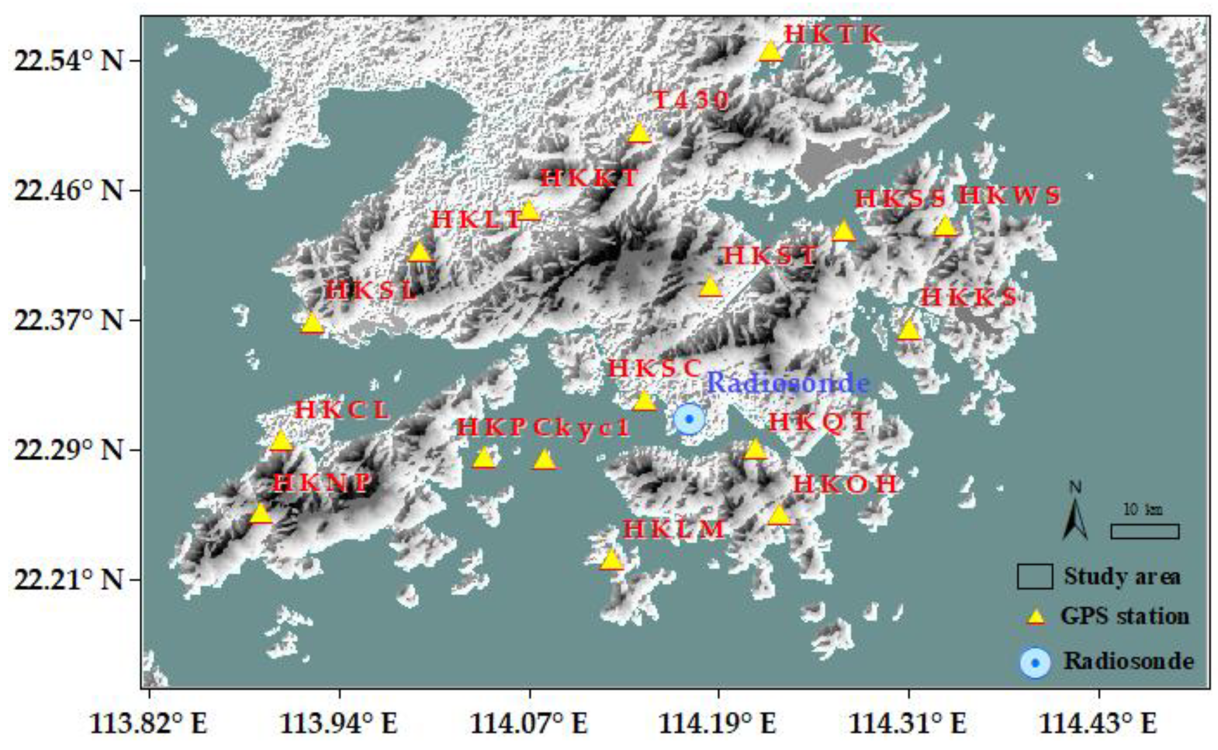
2. Study Area
2.1. GNSS Network in HK
2.2. Radiosonde Station in HK
3. Materials and Methods
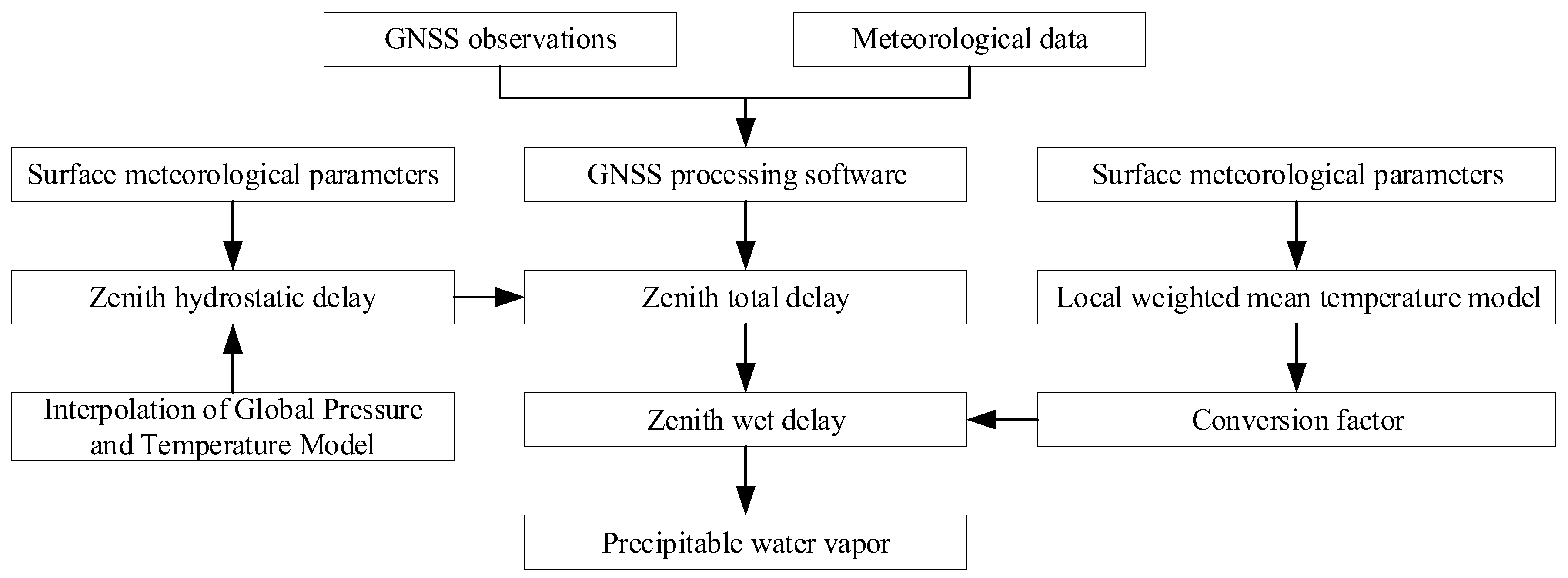
3.1. Method for Water Vapor Retrieval
3.2. Method for Obtaining Tm
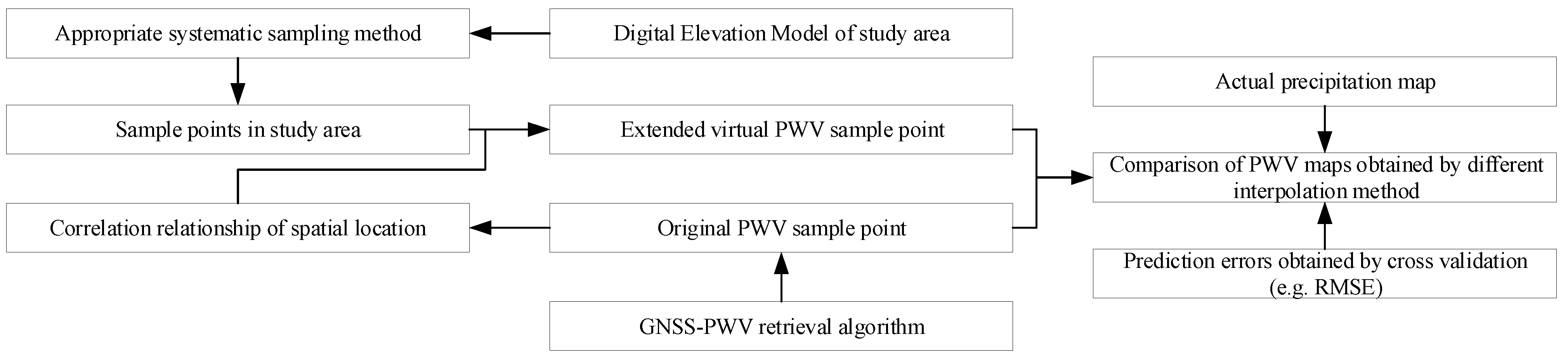
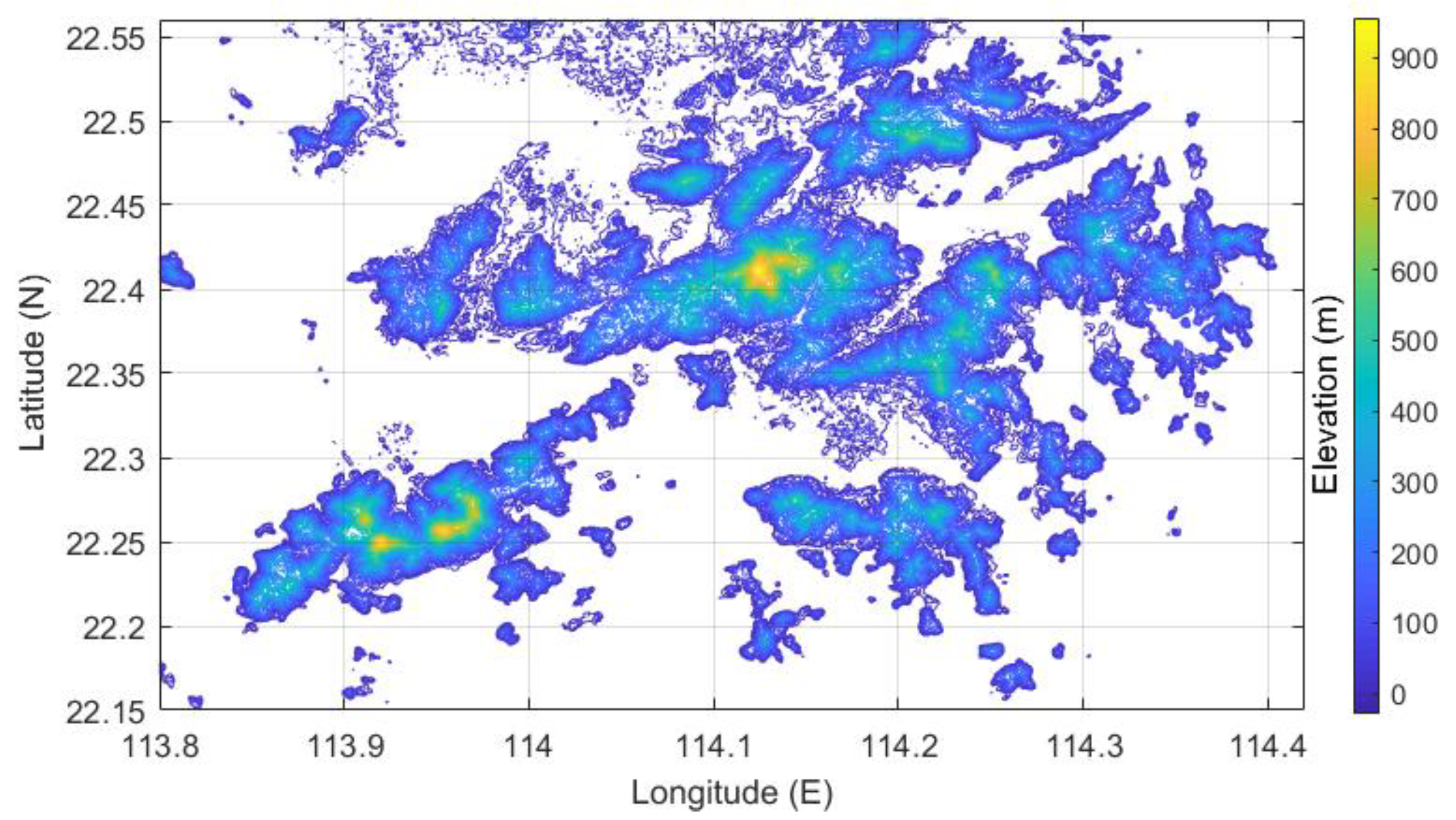
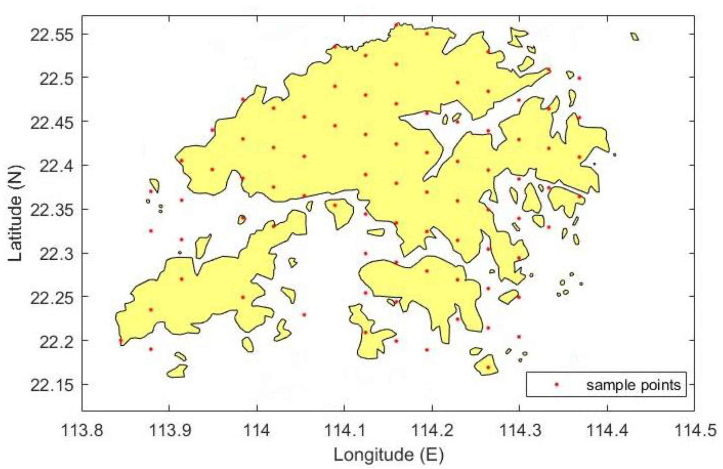
3.3. Method for DEM Point Sampling
- (1)
- Setting the longitude interval to 0.045°, a series of points were determined.
- (2)
- The latitude interval was set to 0.035°, and all points within the scope of the study were determined.
- (3)
- All points in the land area were retained and some points from the oceans were removed on the basis of the points identified above.
3.4. Method for the Establishment of Virtual Sample Points
- (1)
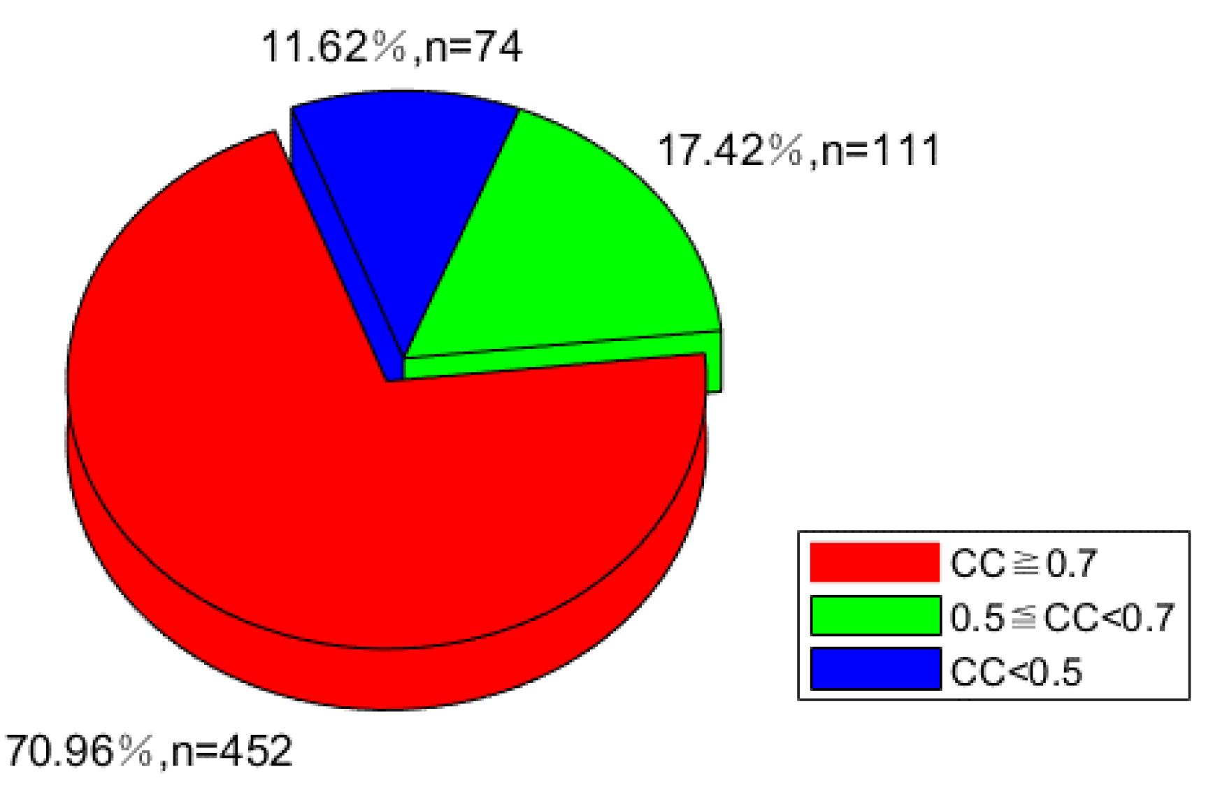
- The CCs between station horizontal position (x, y, x2, y2, and xy)/elevation (h and h2) information and its PWV value were determined. Where x, y, and h represent longitude, latitude, and elevation, respectively.
- (2)
- Station position parameters (e.g. x, y, and h) with CCs of less than 0.7 were deleted.
- (3)
- The PWV expanding functional model based on the linear or nonlinear relations between PWV value and station spatial position information was constructed, and parameters were screened through the stepwise regression method:where and are coefficient column vectors and constant row vectors of variables , respectively. Eventually, the optimal multiple regression equation is deduced by the stepwise method at the significance level of 0.05.
3.5. Method for Spatial Interpolation
- (1)
- Mean error (ME) is the averaged difference between the predicted and measured values. Values close to 0 are preferred. The equation for ME is as follows:where and are the predicted and measured values at location Si, respectively, and n is the number of the sample points.
- (2)
- Root mean square error (RMSE) is also the deviation between the predicted and measured values. Small RMSE values indicate improved accuracy. This index is calculated as follows:
- (3)
- Root mean square standardized error (RMSSE) can be also used to evaluate the quality of a set of prediction. The value of this factor should be close to 1 if the prediction standard errors are valid. Values close to 1 are indicative of good prediction accuracy. Equation (13) shows the equation of this factor:where is the variance of the prediction at location Si.
4. Experiments and Results
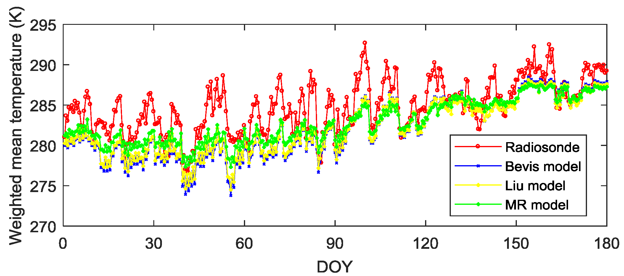
4.1. Modeling of the Regional Tm for HK
4.2. Analysis of the Proposed Tm Model
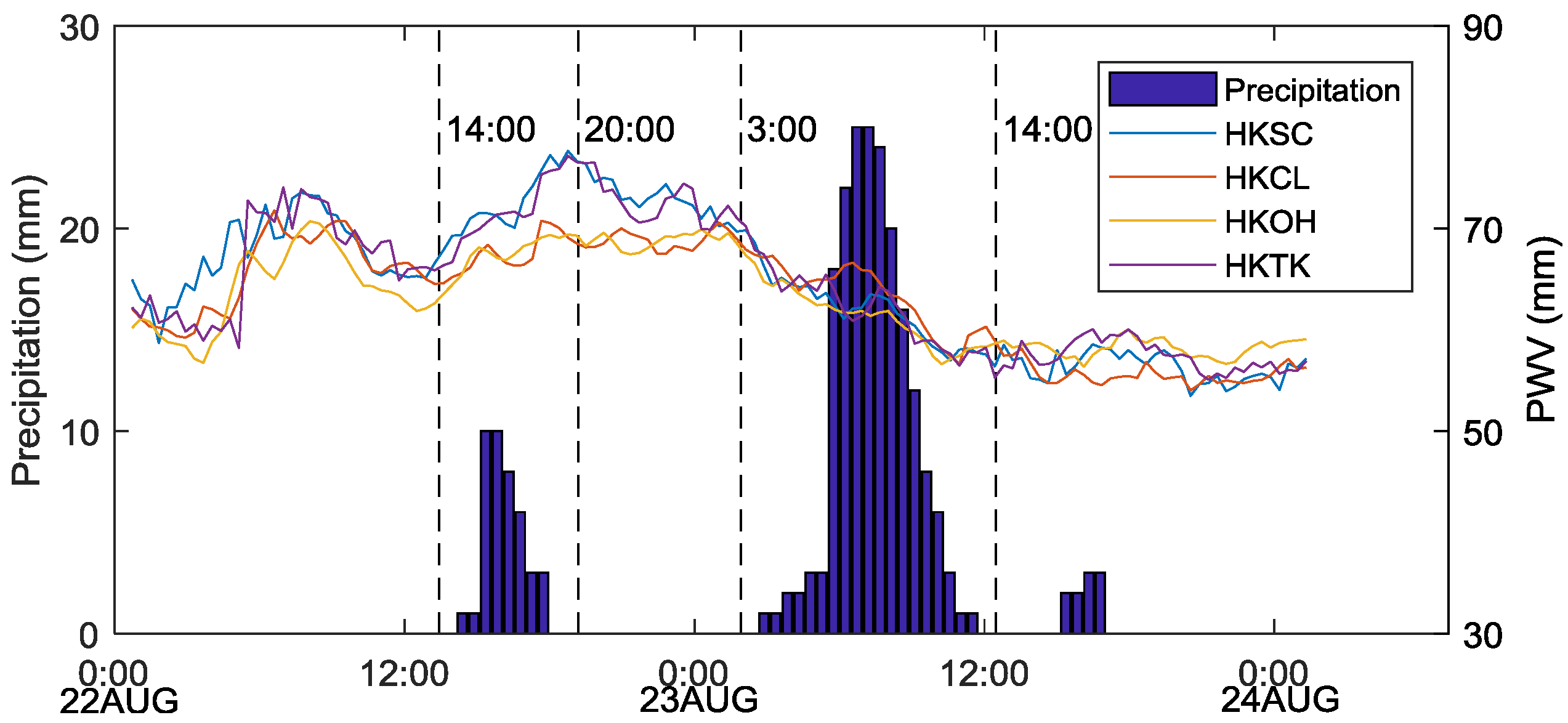
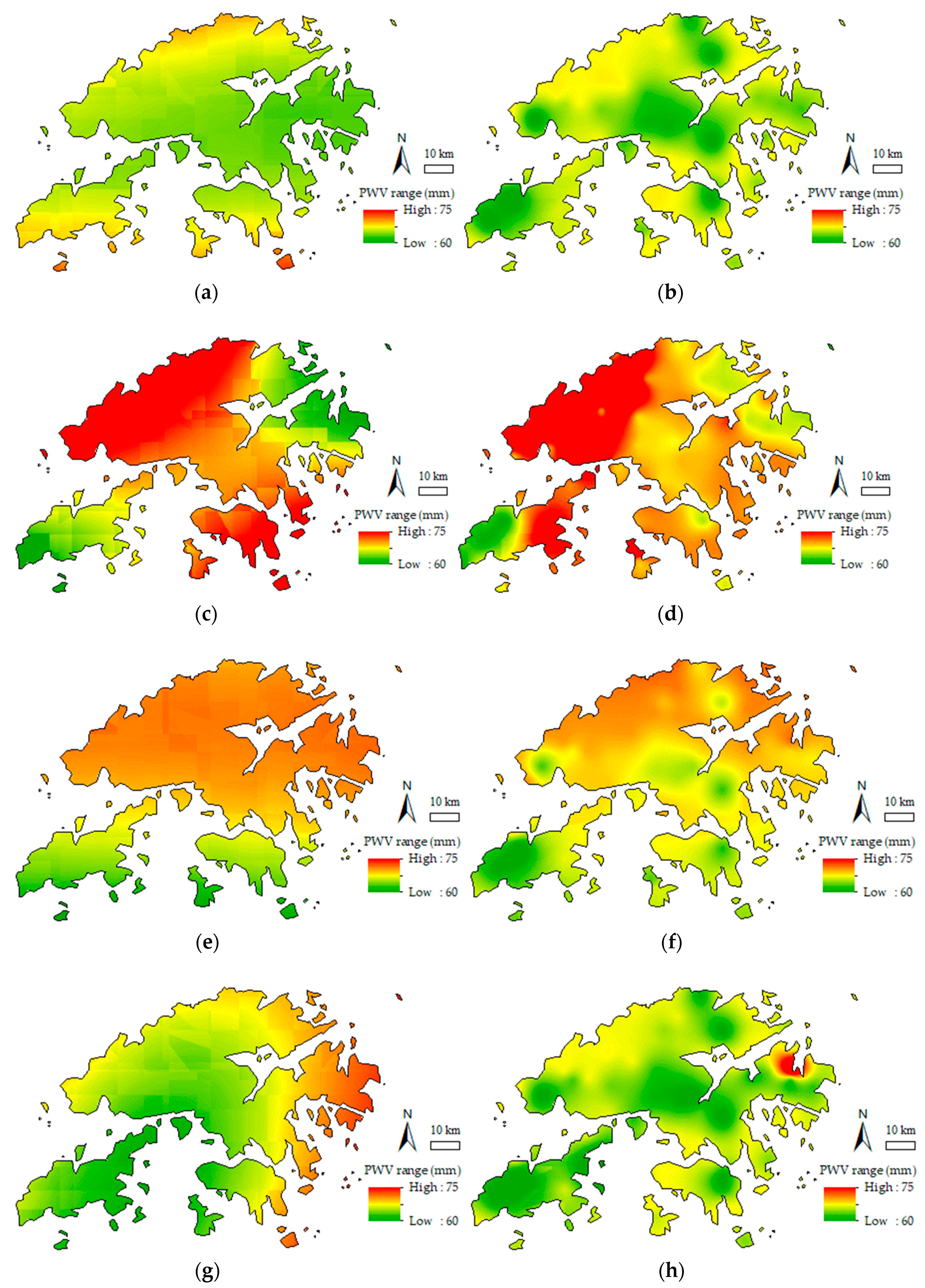
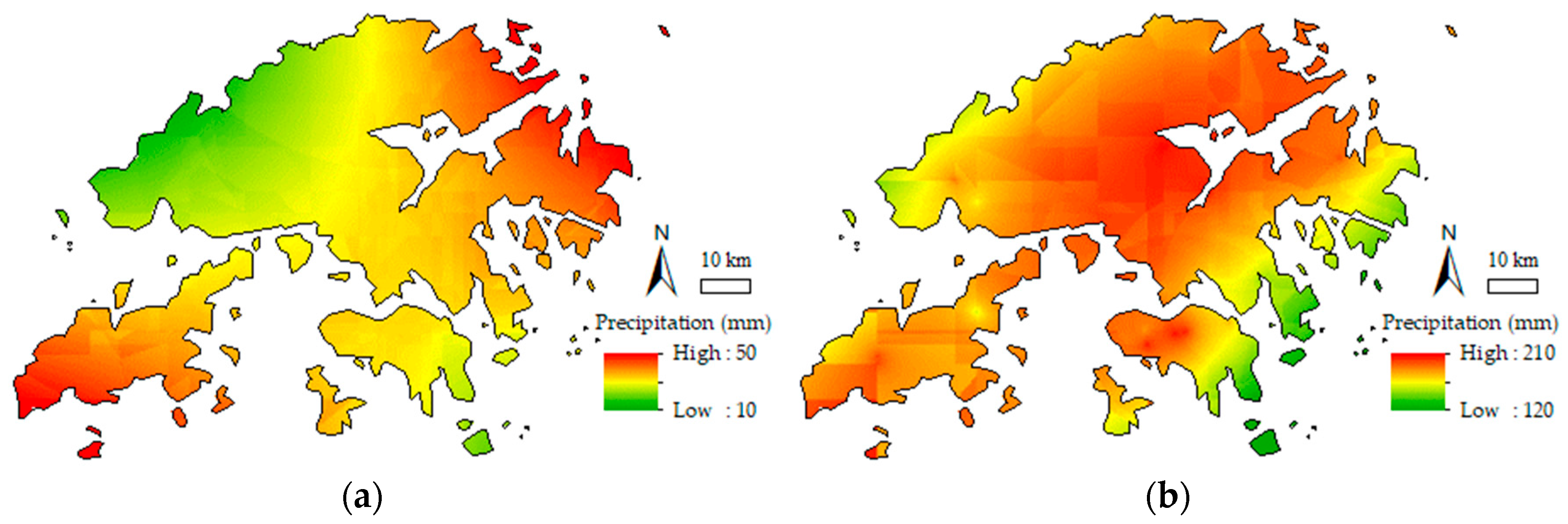
4.3. PWV Spatial Interpolation and Precipitation Distribution Maps
4.4. Error Analysis of the Two Interpolation Schemes
5. Summary and Discussion
Author Contributions
Funding
Acknowledgments
Conflicts of Interest
References
- Torres, B.; Cachorro, V.E.; Toledano, C.; Galisteo, J.P.O.D.; Berjón, A.; de Frutos, A.M.; Bennouna, Y.; Laulainen, N. Precipitable water vapor characterization in the Gulf of Cadiz region (southwestern spain) based on Sun photometer, GPS, and radiosonde data. J. Geophys. Res. 2010, 115, D18103. [Google Scholar] [CrossRef]
- Mattar, C.; Sobrino, J.A.; Julien, Y.; Morales, L. Trends in column integrated water vapour over Europe from 1973 to 2003. Int. J. Climatol. 2011, 31, 1749–1757. [Google Scholar] [CrossRef]
- Bevis, M.; Businger, S.; Herring, T.A.; Rocken, C.; Anthes, R.A.; Ware, R.H. GPS meteorology: Remote sensing of atmospheric water vapor using the global positioning system. J. Geophys. Res. 1992, 97, 15787–15801. [Google Scholar] [CrossRef]
- Holloway, C.E.; Neelin, J.D. Temporal relations of column water vapor and tropical precipitation. J. Atmos. Sci. 2010, 67, 1091–1105. [Google Scholar] [CrossRef]
- Jin, S.; Park, J.-U.; Cho, J.-H.; Park, P.-H. Seasonal variability of GPS-derived zenith tropospheric delay (1994–2006) and climate implications. J. Geophys. Res. 2007, 112, D09110. [Google Scholar] [CrossRef]
- Dai, A.; Wang, J.; Ware, R.H.; Van Hove, T. Diurnal variation in water vapor over North America and its implications for sampling errors in radiosonde humidity. J. Geophys. Res. 2002, 107, 4090. [Google Scholar] [CrossRef]
- Gurbuz, G.; Jin, S. Long-time variations of precipitable water vapour estimated from GPS, MODIS and radiosonde observations in Turkey. Int. J. Climatol. 2017, 37, 5170–5180. [Google Scholar] [CrossRef]
- Li, Z.; Muller, J.-P.; Cross, P. Comparison of precipitable water vapor derived from radiosonde, GPS, and Moderate-Resolution Imaging Spectroradiometer measurements. J. Geophys. Res. 2003, 108, D20. [Google Scholar] [CrossRef]
- Van Baelen, J.; Aubagnac, J.-P.; Dabas, A. Comparison of near–real time estimates of integrated water vapor derived with GPS, radiosondes, and microwave radiometer. J. Atmos. Ocean. Technol. 2005, 22, 201–210. [Google Scholar] [CrossRef]
- Ohtani, R.; Naito, I. Comparisons of GPS-derived precipitable water vapors with radiosonde observations in Japan. J. Geophys. Res. 2000, 105, 26917–26929. [Google Scholar] [CrossRef]
- Liou, Y.-A.; Teng, Y.-T.; Van Hove, T.; Liljegren, J.C. Comparison of precipitable water observations in the near tropics by GPS, microwave radiometer, and radiosondes. J. Appl. Meteorol. 2001, 40, 5–15. [Google Scholar] [CrossRef]
- Kwon, H.-T.; Iwabuchi, T.; Lim, G.-H. Comparison of precipitable water derived from ground-based GPS measurements with radiosonde observations over the Korean Peninsula. J. Meteorol. Soc. Jpn. 2007, 85, 733–746. [Google Scholar] [CrossRef]
- Ding, M. A neural network model for predicting weighted mean temperature. J. Geodesy. 2018, 92, 1187–1198. [Google Scholar] [CrossRef]
- Yao, Y.; Xu, C.; Zhang, B.; Cao, N. GTm-III: A new global empirical model for mapping zenith wet delays onto precipitable water vapour. Geophys. J. Int. 2014, 197, 202–212. [Google Scholar] [CrossRef]
- Böhm, J.; Möller, G.; Schindelegger, M.; Pain, G.; Weber, R. Development of an improved empirical model for slant delays in the troposphere (GPT2w). GPS Solut. 2014, 19, 433–441. [Google Scholar] [CrossRef]
- Liu, Y.; Chen, Y.; Liu, J. Determination of weighted mean tropospheric temperature using ground meteorological measurement. Geo-Spat. Inf. Sci. 2001, 4, 14–18. [Google Scholar]
- Wang, J.; Zhang, L.; Dai, A. Global estimates of water-vapor-weighted mean temperature of the atmosphere for GPS applications. J. Geophys. Res. 2005, 110, D21. [Google Scholar] [CrossRef]
- Wang, X.; Zhang, K.; Wu, S.; Fan, S.; Cheng, Y. Water vapor-weighted mean temperature and its impact on the determination of precipitable water vapor and its linear trend. J. Geophys. Res. Atmos. 2016, 121, 833–852. [Google Scholar] [CrossRef]
- Bordi, I.; Raziei, T.; Pereira, L.S.; Sutera, A. Ground-based GPS measurements of precipitable water vapor and their usefulness for hydrological applications. Water Resour. Manag. 2015, 29, 471–486. [Google Scholar] [CrossRef]
- Li, L.; Yuan, Z.; Luo, P.; Shen, J.; Long, S.; Zhang, L.; Jiang, Z. A system developed for monitoring and analyzing dynamic changes of GNSS precipitable water vapor and its application. In Proceedings of the China Satellite Navigation Conference, Xian, China, 13–15 May 2015. [Google Scholar]
- Chen, B.; Dai, W.; Liu, Z.; Wu, L.; Kuang, C.; Ao, M. Constructing precipitable water vapor map from regional GNSS network observations without collocated meteorological data for weather forecasting. Atmos. Meas. Tech. 2018, 11, 5153–5166. [Google Scholar] [CrossRef]
- Xuan, T.N.; Ba, T.N.; Khac, P.D.; Quang, H.B.; Thi, N.T.N.; Van, Q.V.; Thanh, H.L. Spatial interpolation of meteorologic variables in vietnam using the kriging method. J. Inf. Proc Syst. 2015, 11, 134–147. [Google Scholar]
- Wardah, T.; Sharifah Nurul Huda, S.Y.; Deni, S.M.; Nur Azwa, B. Radar rainfall estimates comparison with kriging interpolation of gauged rain. In Proceedings of the 2011 IEEE Colloquium on Humanities, Science and Engineering, Penang, Malaysia, 5–6 December 2011. [Google Scholar]
- Berndt, C.; Haberlandt, U. Spatial interpolation of climate variables in Northern Germany—Influence of temporal resolution and network density. J. Hydrol. 2018, 15, 184–202. [Google Scholar] [CrossRef]
- Setiyoko, A.; Arymurthy, A.M.; Arief, R. Effects of different sampling densities and pixel size on kriging interpolation for predicting elevation. In Proceedings of the 2018 International Conference on Signals and Systems (ICSigSys), Bali, Indonesia, 1–3 May 2018. [Google Scholar]
- Bradley, S.G.; Dirks, K.N.; Stow, C.D. High resolution studies of rainfall on Norfolk Island, Part III: A model for rainfall redistribution. J. Hydrol. 1998, 208, 194–203. [Google Scholar] [CrossRef]
- Realini, E.; Sato, K.; Tsuda, T.; Oigawa, M.; Iwaki, Y.; Shoji, Y.; Seko, H. Local-Scale precipitable water vapor retrieval from high-elevation slant tropospheric delays using a dense network of GNSS receivers. In IAG 150 Years; Springer: Berlin/Heidelberg, Germany, 2015; pp. 485–490. [Google Scholar]
- Saastamoinen, J. Contributions to the theory of atmospheric refraction. Bulletin Géodésique 1972, 105, 279–298. [Google Scholar] [CrossRef]
- Li, G.; Wang, H. Using GAMIT to derive the precipitabel water vapor. In Proceedings of the 2010 International Conference on Multimedia Technology, Ningbo, China, 29–31 October 2010. [Google Scholar]
- Wang, Z.; Xin, P.; Li, R.; Wang, S. A Method to reduce non-nominal troposphere error. Sensors 2017, 17, 1751. [Google Scholar] [CrossRef] [PubMed]
- Yang, F.; Guo, J.; Shi, J.; Zhou, L.; Xu, Y.; Chen, M. A method to improve the distribution of observations in GNSS water vapor tomography. Sensors. 2018, 18, 2526. [Google Scholar] [CrossRef] [PubMed]
- Mukherjee, S.; Garg, R.D.; Raju, P.L.N. Evaluation of topographic index in relation to terrain roughness and DEM grid spacing. J. Earth Syst. Sci. 2013, 122, 869–886. [Google Scholar] [CrossRef]
- QGIS Software. Available online: https://www.qgis.org/en/site/ (accessed on 18 December 2018).
- Meng, Q.; Liu, Z.; Borders, B.E. Assessment of regression kriging for spatial interpolation—Comparisons of seven GIS interpolation methods. Cartogr. Geogr. Inf. Sci. 2013, 40, 28–39. [Google Scholar] [CrossRef]
- Addink, E.A. A comparison of conventional and geostatistical methods to replace clouded pixels in NOAA-AVHRR images. Int. J. Remote Sens. 1999, 20, 961–977. [Google Scholar] [CrossRef]
- Ashiq, M.W.; Zhao, C.; Ni, J.; Akhtar, M. GIS-based high-resolution spatial interpolation of precipitation in mountain–plain areas of Upper Pakistan for regional climate change impact studies. Theor. Appl. Climatol. 2009, 99, 239–253. [Google Scholar] [CrossRef]
- Bostan, P.A.; Heuvelink, G.B.M.; Akyurek, S.Z. Comparison of regression and kriging techniques for mapping the average annual precipitation of Turkey. Int. J. Appl. Earth Obs. Geoinf. 2012, 19, 115–126. [Google Scholar] [CrossRef]
- Alvarez, O.; Guo, Q.; Klinger, R.C.; Li, W.; Doherty, P. Comparison of elevation and remote sensing derived products as auxiliary data for climate surface interpolation. Int. J. Climatol. 2013, 34, 2258–2268. [Google Scholar] [CrossRef]
- Wang, X.; Song, L.; Dai, Z.; Cao, Y. Feature analysis of weighted mean temperature Tm in Hong Kong. J. Nanjing. Univ. Inf. Sci. Technol. Nat. Sci. Edn. 2011, 3, 47–52. [Google Scholar]
- JASP Software. Available online: https://jasp-stats.org/ (accessed on 18 December 2018).
- Onn, F.; Zebker, H.A. Correction for interferometric synthetic aperture radar atmospheric phase artifacts using time series of zenith wet delay observations from a GPS network. J. Geophys Res. 2006, 111, B9. [Google Scholar] [CrossRef]
- Goovaerts, P. Geostatistical approaches for incorporating elevation into the spatial interpolation of rainfall. J. Hydrol. 2000, 228, 113–129. [Google Scholar] [CrossRef]

| Station Name | Longitude E (°) | Latitude N (°) | Height (m) |
|---|---|---|---|
| HKCL | 113.91 | 22.30 | 7.714 |
| HKKS | 114.31 | 22.37 | 44.718 |
| HKKT | 114.07 | 22.44 | 34.576 |
| HKLM | 114.12 | 22.22 | 8.554 |
| HKLT | 114.00 | 22.41 | 125.922 |
| HKNP | 113.89 | 22.25 | 350.672 |
| HKOH | 114.23 | 22.25 | 166.401 |
| HKPC | 114.04 | 22.28 | 18.130 |
| HKQT | 114.21 | 22.29 | 5.178 |
| HKSC | 114.14 | 22.32 | 20.239 |
| HKSL | 113.93 | 22.37 | 95.297 |
| HKSS | 114.27 | 22.43 | 38.714 |
| HKST | 114.18 | 22.40 | 258.705 |
| HKTK | 114.22 | 22.55 | 22.533 |
| HKWS | 114.34 | 22.43 | 63.791 |
| kyc1 | 114.08 | 22.28 | 116.380 |
| T430 | 114.13 | 22.49 | 41.323 |
| King’s Park (45004) | 114.17 | 22.31 | 66.0 |
| Parameter | Strategy |
|---|---|
| Interval Zen/Number Zen | 1/25 |
| Elevation Cutoff | 10° |
| Mapping Function | VMF1 |
| CC | Tm | Ts | e | P |
|---|---|---|---|---|
| Tm | 1 | 0.862 | 0.833 | −0.744 |
| Ts | 0.862 | 1 | 0.926 | −0.851 |
| e | 0.833 | 0.926 | 1 | −0.843 |
| P | −0.744 | −0.851 | −0.843 | 1 |
| Model | R | R2 | S.E |
|---|---|---|---|
| 1 | 0.862 | 0.743 | 1.932 |
| 2 | 0.867 | 0.752 | 1.901 |
| Evaluation Indices | MR Model | Liu Model | Bevis Model |
|---|---|---|---|
| RMSE | 2.8 | 3.3 | 3.5 |
| ΔRMSE | 0.9% | 1.1% | 1.2% |
| Time Epoch | ME | RMSE | RMSSE | |||
|---|---|---|---|---|---|---|
| Scheme I | Scheme II | Scheme I | Scheme II | Scheme I | Scheme II | |
| 1 | 0.18 | 0.05 | 5.63 | 3.09 | 1.25 | 1.02 |
| 2 | −0.18 | −0.05 | 10.62 | 5.58 | 1.35 | 0.97 |
| 3 | 0.02 | −0.01 | 3.23 | 1.61 | 1.61 | 1.02 |
| 4 | 0.25 | 0.02 | 6.37 | 2.54 | 1.47 | 1.02 |
| Mean | 0.07 | 0.01 | 6.47 | 3.20 | 1.42 | 1.01 |
© 2019 by the authors. Licensee MDPI, Basel, Switzerland. This article is an open access article distributed under the terms and conditions of the Creative Commons Attribution (CC BY) license (http://creativecommons.org/licenses/by/4.0/).
Share and Cite
Liu, C.; Zheng, N.; Zhang, K.; Liu, J. A New Method for Refining the GNSS-Derived Precipitable Water Vapor Map. Sensors 2019, 19, 698. https://doi.org/10.3390/s19030698
Liu C, Zheng N, Zhang K, Liu J. A New Method for Refining the GNSS-Derived Precipitable Water Vapor Map. Sensors. 2019; 19(3):698. https://doi.org/10.3390/s19030698
Chicago/Turabian StyleLiu, Chen, Nanshan Zheng, Kefei Zhang, and Junyu Liu. 2019. "A New Method for Refining the GNSS-Derived Precipitable Water Vapor Map" Sensors 19, no. 3: 698. https://doi.org/10.3390/s19030698
APA StyleLiu, C., Zheng, N., Zhang, K., & Liu, J. (2019). A New Method for Refining the GNSS-Derived Precipitable Water Vapor Map. Sensors, 19(3), 698. https://doi.org/10.3390/s19030698