Abstract
This study deals with the problem of covariance matrix estimation for radar sensor signal detection applications with insufficient secondary data in non-Gaussian clutter. According to the Euclidean mean, the authors combined an available prior covariance matrix with the persymmetric structure covariance estimator, symmetric structure covariance estimator, and Toeplitz structure covariance estimator, respectively, to derive three knowledge-aided structured covariance estimators. At the analysis stage, the authors assess the performance of the proposed estimators in estimation accuracy and detection probability. The analysis is conducted both on the simulated data and real sea clutter data collected by the IPIX radar sensor system. The results show that the knowledge-aided Toeplitz structure covariance estimator (KA-T) has the best performance both in estimation and detection, and the knowledge-aided persymmetric structure covariance estimator (KA-P) has similar performance with the knowledge-aided symmetric structure covariance estimator (KA-S). Moreover, compared with existing knowledge-aided estimator, the proposed estimators can obtain better performance when secondary data are insufficient.
1. Introduction
Covariance matrix estimation plays an important role in advanced radar sensor signal processing algorithms such as space–time adaptive processing (STAP) [1] and adaptive signal detection [2,3,4,5,6]. In the homogeneous Gaussian environment, the sample covariance matrix (SCM) estimator [7] is the maximum likelihood estimate (MLE) [8]. However, in many situations, the clutter is not Gaussian distributed. In K-distributed clutter, a special case of compound-Gaussian distributed clutter, the normalized SCM (NSCM) estimator [9] is often used to estimate the actual covariance matrix. In correlated heavy-tailed clutter, the approximate maximum likelihood (AML) estimator [10,11] was derived, which is an iterative solution of covariance matrix, as well as a unified method of the SCM and NSCM estimator. In a partially homogeneous clutter environment, an iterative method was provided to calculate the weighting coefficients of each covariance matrix of secondary data vector [12].
Recently, a covariance estimate based on the geometric means and medians was proposed in the open literature. In [13,14], the authors used five difference geometric means (Euclidean mean, Log–Euclidean mean, Root–Euclidean mean, Power-Euclidean mean, and Cholesky mean) to obtain the corresponding covariance estimators without considering the clutter distribution. In [15], the authors used the geometric means and medians to obtain the estimators and obtained the corresponding detectors. Using geometric methods can obtain the non-linear model between primary data covariance matrix and secondary data covariance matrix which can further improve the covariance estimation accuracy. However, in the real world, above methods will suffer from the sample-starvation effect, namely, we may not obtain sufficient secondary data samples to estimate an accurate covariance matrix. Precisely, to ensure the loss within 3 dB, the required number of secondary data are near twice the number of the system degrees of freedom (DOF), according to the Reed, Mallett, and Brennan (RMB) [16] criterion.
In order to alleviate the sample-starvation effect, a priori knowledge of the clutter covariance matrix is a possible way to improve covariance matrix estimation accuracy [17]. The knowledge-aided (KA) technology, as an important part of a cognitive radar system [18], has been widely used in the secondary data selection [19], detector design [20,21,22], and covariance matrix estimation [23,24,25]. The essence of KA method is to use the prior information to reduce the DOF of covariance matrix estimation, and hence obtain a more accurate result in small sample case [26].
The KA covariance estimation methods can fall loosely into three categories based on the difference of knowledge. The first category of knowledge is the structure information of covariance matrices, such as symmetric spectrum [21,27], persymmetry structure [20,22,28] and identity matrix [29,30,31]. The second category of knowledge is the prior statistical distribution knowledge of the data of covariance matrix, such as the Wishart or inverse Wishart distributed [32,33,34]. The third category of knowledge is the data of environment, such as synthetic aperture radar (SAR) imagery [35], physics-based models [36], digital elevation model (DEM) [37], and history or simulation data of clutter [38,39].
The structure of the covariance matrix can reduce the covariance matrix degree of freedom, thereby reducing the dependence on the number of samples. Data of the environment can be used to obtain an a priori clutter covariance matrix and utilize this covariance matrix combined with the SCM estimator to obtain a more accurate one, which is usually in the form of color-loaded version. The color-loaded methods can result in the linear combination of the prior covariance matrix and the SCM estimator. The key issue of these methods is to determine the weighting factor. In the Gaussian environment, Ref. [23] used the convex combination (CC) of the prior covariance estimator and SCM estimator and obtained the weighting factor via solving a convex optimization problem. In [24], the authors used a maximum likelihood (ML) estimator approach to obtain the optimal weighting factor via a search method in the Gaussian environment. These methods are based on a Gaussian distribution to obtain the weighting factor but the real world is not always Gaussian. Therefore, existing KA methods can solve the sample-starvation problem but they will suffer from loss due to model mismatch when the clutter is non-Gaussian [40,41,42].
In addition, another class of color-loaded methods use the Bayes framework to obtain covariance matrix estimation. These methods [43,44,45] assumed the covariance matrix follows some prior distributions such as Winshart [17] and inverse-Winshart [34] distribution and use the prior covariance matrix as the mean value of the distributions to caculate the maximum posterior probability (MAP) estimation of the covariance.
In this paper, we use the linear combination of the prior covariance matrix and the estimated covariance matrix to obtain the knowledge-aided covariance estimators. It is different with the Bayes knowledge-aided covariance estimators which need assume the prior distribution of covariance. The main contribution in this work is a new method to calculate the weighting factor and combining the prior covariance with the structured covariance estimator via the new method to obtain three knowledge-aided structured covariance estimators. We show that the proposed estimators can use knowledge effectively and have a better estimation and detection performance both in Gaussian and non-Gaussian clutter when secondary data are insufficient. These results are valiadted by numerical experiments and real sea clutter data collected by the IPIX radar sensor system.
2. Problem Formulation
In this section, we derive some classic covariance estimators from the view of the Euclidean metric. First, we formulate the signal model. Then, we obtain the classic covariance estimators via Euclidean mean.
2.1. Data Model
Consider a set of received radar sensor data where the cell under test (CUT) and secondary data share the same covariance structure. Specifically, denoted by , , , the dimensional random vectors. Assuming and are complex circular multivariate compound-Gaussian distributed, which can be expressed as [46,47]
where and are positive and possibly random numbers, named the texture component, determing the local scattering power, and is modeled as dimensional circularly symmetric zero-mean vectors with positive definite covariance matrix
where denotes the conjugate transpose operator and denotes the statistical expectation. Therefore, the conditional covariance matrix of and for a given , are and , respectively.
2.2. Euclidean Mean
From the geometry metric perspective, the Frobenius normal of two matrices is the Euclidean distance between them, namely
where denotes the Euclidean distance.
In number field, for a set of K positive numbers , the mean is the minimum value of the sum of the squared distance to the given points
In the geometry field, the mean for a finite set of Hermitian positive definite (HPD) matrices origins from generalized mean for positive numbers. Pennec [48] defined the geometry means, and obtained the geometric mean using a gradient descent algorithm. Pennec proved that the geometry means for a set of HPD matrices exist and unique. Therefore, the Euclidean mean associated with Euclidean distance (3), of a set of K HPD matrices , is defined by
Then, the Euclidean mean can be derived by differentiating
It is noted that Equation (6) is the SCM estimator or the NSCM estimator when or , respectively. The SCM estimator and the NSCM estimator are obtained based on Gaussian clutter and non-Gaussian clutter, respectively. Therefore, in the Euclidean metric case, covariance estimate methods based on probability distributed are equivalent to the geometric metric methods. Moreover, to eliminate the effect of texture components and , like the NSCM, we normalized the received data vectors, namely,
where is the moment estimation of texture component [9,11].
In the Gaussian clutter, and are constant and equal to each other, the SCM estimator is the maximum estimation (ML) estimator of the CUT. In the compound-Gaussian clutter, and are positive random variables and usually unequal, and the SCM estimator suffers from the serious performance loss. In contrast, the NSCM can perform well in such an environment. However, to ensure the loss within 3 dB, both of these estimators should follow the RMB criterion. Unfortunately, in the real world, the secondary data are always insufficient which reduces the estimation performance of the SCM and NSCM estimators. Using prior knowledge can solve this problem effectively. In the next section, we provide a new knowledge-aided covariance estimate method via Euclidean metric.
3. Proposed Estimators
In this section, we derive our covariance estimator. We use the linear combination as the covariance estimation model. The covariance estimation model of each cell is modeled as [23]
where is the prior covariance matrix of CUT, which can be obtained from the SAR imagery [35], physics-based models [36], digital elevation model (DEM) [37] and history or simulation data [38,39], and is the weighting factor. Then substituting Equation (8) into Equation (5)
First, taking the derivative of Equation (9) with respect to results in
Second, taking the derivative of Equation (9) with respect to and nulling the result, we obtain (See Appendix A for a detailed derivation)
where is the Euclidean mean of .
It is noted that when and we can rewrite as
where . And Equation (12) is similar with the Equation (20) in [23].
In this study, we use structure information to improve the estimation accuracy of and . This structure information can be obtained via prior knowledge.
- Persymmetric covariance matrixFor a radar sensor system using a symmetrically spaced linear array with constant pulse repetition interval, the covariance matrix has the persymmetric structure [49]. This structure information yields the estimate [28]andwhere denotes complex conjugate, and is the permutation matrix, i.e.,
- Symmetric covariance matrixFor a temporal steering and fixed radar sensor system, the symmetric property of the clutter power spectral density (PSD) is always present [21]. This structure information yields the estimateandwhere denotes the real part of .
- Toeplitz covariance matrixIf the data obtained by sampling a spatially stationary noise field with a uniform linear array, then the Toeplitz structure exists [50]. The Toeplitz structure covariance matrix can be calculated as [15]where is the correlation coefficient. is a Toeplitz matrix with . According to the ergodicity of a wide-sense stationary, the correlation coefficient of data can be calculated by averaging over time instead of its statistical expectation, aswhere is the nth element of ,
Hence, we obtain three knowledge-aided estimators via three structure information, namely, the knowledge-aided persymmetric covariance estimator (KA-P), the knowledge-aided symmetric covariance estimator (KA-S) and the knowledge-aided Toeplitz covariance estimator (KA-T). The detailed calculation method is shown in Table 1.

Table 1.
Three knowledge-aided structured covariance estimators.
4. Performance Assessment
In this section, we analyze the estimation and detection performance of the proposed estimators with the existing SCM [7], CC [23] and ML [24] estimators. First, we compare estimation performance of the proposed estimators with the existing estimators. Second, we use the adaptive normalized matched filter (ANMF) detector [51,52] with each estimator to further illustrate the detection performance of the proposed estimators. All of these performance analyses are simulated in Gaussian and compound-Gaussian clutter. Finally, we analyze the detection performance via real sea clutter data collected by the IPIX radar sensor system. In all simulations, we consider a coherent pulse train of for reducing computation burden.
The prior covariance matrix is taken as a perturbed matrix of the actual matrix and can be generated by [24]
where ⊙ denotes the Hadamard matrix product, and is a vector of independent and identically distributed (IID) Gaussian random variables with mean 1 and variance . The perturbed vector determines the effectiveness of the prior covariance matrix , when the variance is large (), the can be regarded as an invalid prior covariance matrix and the weighting factor will become small, while the variance is small the can be regarded as an effective prior covariance matrix and the weighting factor will become large.
The one-lag correlation coefficient and normalized doppler of clutter are used to simulate the covariance matrix of clutter
The texture component of compound-Gaussian clutter in each cell, namely , follows the inverse gamma distribution [47,53] with shape parameter and scale parameter , i.e.,
4.1. Estimation Performance
In this section, we use the simulation data to measure the estimation performance of our estimators. First, we compare the estimation value of weighting factor under difference secondary data and clutter environment. Second, we calculate the normalized Frobenius norm (NFN) of the error matrix [11] to display the estimation accuracy of the estimators.
Figure 1 illustrates that for the proposed estimators, the clutter environment and the number of secondary data have a little impact on the weighting factor. The proposed estimators are more sensitive to . When becomes large becomes small to keep the estimation accuracy. Therefore, the proposed estimators have the robust estimate property. The change in of the KA-P and KA-S estimators show that these two estimators have similar performance in estimation. For the CC and ML estimators, the clutter environment has a significant impact on the weighting factor. Especially, in the compound-Gaussian clutter (Figure 1a,b), though the prior covariance matrix is accurate the weighting factor of the CC and ML is small. Therefore, the CC and ML estimators can not make the most of the prior knowledge under the compound-Gaussian clutter. Moreover, as the increases, all the estimators tend to abandon the inaccurate prior knowledge. Therefore, all the KA methods can recognize the invalid knowledge.
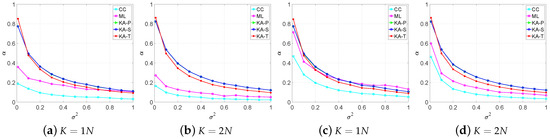
Figure 1.
Estimation values of α under different values of the perturbation level clutter, (a,b) in compound-Gaussian clutter; (c,d) in Gaussian clutter.
Next, we measure the estimation accuracy by calculating the NFN of the error matrix, defined as [11]
where can be replaced by , , , , [23] and [24].
We calculate the mean of 1000 Monte Carlo experiments of the NFN to obtain the NFN estimation values of each estimator, shown in Figure 2. From the estimation error results in the compound-Gaussian clutter (Figure 2a–d), we find that the SCM estimator suffers from significant performance loss, and hence the CC and ML estimators using the SCM as the basic estimator have serious estimation error, though the is small. For the proposed estimators, in the compound-Gaussian clutter, the KA-T estimator has the smallest estimation error, which suggests that the KA-T has the best detection performance among the proposed estimator. Compared with the SCM, CC and ML estimators, the proposed estimators have better estimation accuracy than them in the compound-Gaussian clutter. In the Gaussian clutter (Figure 2e–h), the estimators have similar estimation accuracy when . When , the proposed estimators have better estimate results than the SCM, CC and ML estimators.
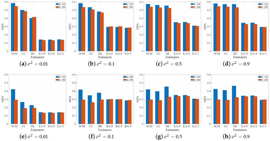
Figure 2.
NFN under different values of the perturbation level (a–d) in compound-Gaussian clutter; (e–h) in Gaussian clutter.
In general, from Figure 2, when in the Gaussian clutter and the number of secondary data are sufficient, all three estimators have similar estimation performance. In other cases, the proposed estimators are better than the SCM, CC and ML estimators. Moreover, among proposed estimators, the KA-T estimator provides the best estimate.
4.2. Detection Performance
To further illustrate the effectiveness of our estimators, we address the problem of detecting a known complex signal vector in received data vector, which can be formulated as a binary hypotheses test
where , a is an unknown deterministic parameter, which accounts for both the target and the channel effects. is the normalized frequency of the target and set to be .
Then, we use the ANMF detector to analyse the detection performance of our proposed covariance estimators. The structure of ANMF detector is defined as [51,52]
where is the threshold of ANMF, can be replaced by , , , , and .
The standard Monte Carlo technique based on 100/PFA independent trails is utilized to obtain the decision thresholds for a given probability of false alarm PFA. In this paper, to alleviate the computational burden. The detection probabilities (PD) are computed via 100,000 Monte Carlo experiments. In the compound-Gaussian case, the signal-to-clutter ratio (SCR) is defined as [47]
where for . In the Gaussian case, we set .
The sensor detection results are shown as Figure 3 and Figure 4 in the compound-Gaussian and Gaussian environments, respectively. It is shown that the detection performance of the proposed estimators are better than that of the other three estimators in most cases. In the compound-Gaussian case (Figure 3), compared with the ML estimator, the ANMF detector with proposed estimators have a significant advantage when secondary data are insufficient. When and , the detection performance of the ML estimator is close to the KA-P and KA-S estimators. For the CC estimator, it is more robust than the ML estimator when . But compared with proposed estimators, it still suffers much detection loss because of the non-Gaussian clutter. When prior knowledge is accurate, e.g., , the three proposed estimators have nearly the same detection performance. When the prior knowledge becomes coarse, the detection performance of proposed estimators begin to differentiate. The best is the KA-T estimator, followed by the KA-S and KA-P estimator.
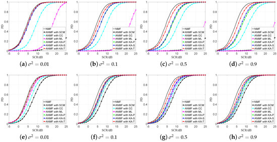
Figure 3.
PD versa SCR with different values of the perturbation level in compound-Gaussian clutter PFA = 10−3, (a–d) K = 1N; (e–h) K = 2N.
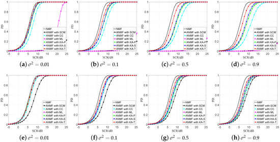
Figure 4.
PD versa SCR with different values of the perturbation level in Gaussian clutter PFA = 10−3, (a–d) K = 1N; (e–h) K = 2N.
The sensor detection results in the Gaussian clutter case is shown in Figure 4. The proposed estimators have better performance when the secondary data are insufficient because the proposed estimators can use the prior knowledge more effectively which can be found in Figure 1c. When the secondary data are sufficient, all the KA estimators have similar detection performance, but the KA-T estimator still has a small advantage.
From Figure 3 and Figure 4, we find that the proposed estimators have better detection performance than the SCM, CC and ML estimators, especially under the sample starvation situation. The ML and SCM estimators are sensitive to the number of secondary data, while the CC estimator has relatively robust property in secondary data changing. Among the proposed estimators, the KA-T has the best detection performance, which is similar to the result in Figure 1 and Figure 2.
4.3. IPIX Radar Sensor System Data
In this section, we use the ANMF detector with the KA-P, KA-S, KA-T, SCM, CC and ML estimators with one set of real data collected by the McMaster IPIX radar sensor system. The IPIX radar sensor system is a transportable experimental radar system designed and constructed at McMaster University.
A detailed statistical analysis of the adopted real data has been conducted in [38,54,55,56]. We use the 19980223_170435_ANTSTEP.CDF data, which consists of 60,000 coherent pulse trains and 34 range cells, to analyze the proposed detector. The sensor system measurements were collected in winter 1998 using the McMaster IPIX radar in Grimsby, on the shore of Lake Ontario, between Toronto and Niagara Falls. This sensor system is a fully coherent X-band radar, with advanced features such as dual transmit/receive polarization, frequency agility, and stare/surveillance mode. Moreover, it has been upgraded since the measurement of the Dartmouth data in 1993. More specifically, the dynamic range has been improved from 8 bits to 10 bits, so that strong target and weak clutter signals can be observed simultaneously without clipping or large quantization error. The sensor system parmeters are shown in Table 2.
Table 2.
The system parameters of the IPIX radar sensor.
The Range–Doppler image is shown as Figure 5.
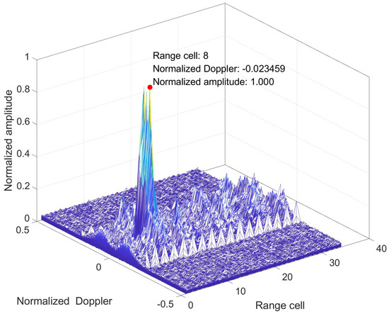
Figure 5.
Range–Doppler image of IPIX clutter data.
It is shown that the strongest clutter appear at the 8th range cell. Therefore, we choose the 8th range cell as the CUT, exploiting surrounding cells as training data. Moreover, because of the normalized Doppler of clutter is near zero and radar transmits the coherent pulses, the covariance meets the prior condition of symmetry, persymmetry and Toeplitz structure. We apply the statistical tests for all the available temporal samples, the total number of different windows is . According to [53], we use the MLE to estimate and .
For the prior covariance, the SAR imagery [35] and digital elevation model (DEM) [37] are not always getatable, physics-based models [36] may have model mismatch. Compared with above prior knowledge, the historical environment data are more accessible and timely. Therefore, according to [33,57], we use the previous temporal samples of current CUT as the historical measure data to estimate 100 covariance matrices. Then, we obtain the prior knowledge covariance matrix of the CUT via calculating the mean of the 100 covariance matrices. As shown in Figure 6, we slide the window to obtain the ith covariance matrix estimation , namely
where is the ith sliding normalized vector in the CUT. Then, we average all of to obtain the prior knowledge covariance matrix
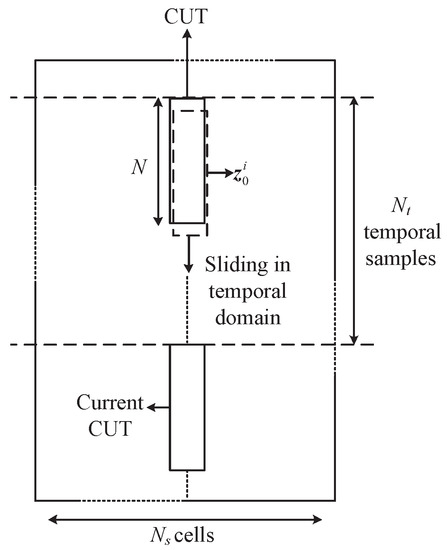
Figure 6.
Procedure for estimating .
After the above process, we add a point target in the 8th range cell for different SCRs and set the normalized Doppler of the target as . We use the first 50,000 pulses via standard Monte Carlo technique to obtain the detection thresholds for a given probability of false alarm () and use the remaining 10,000 pulses to obtain the PD of each detector.
The sensor detection results are shown in Figure 7. Like the simulation results, the ANMF detector with the ML estimator is sensitive to the number of secondary data. When the ANMF detector with the ML estimator and the ANMF detector with the SCM estimator are fail to detect the target. While, the proposed estimators and the CC estimator work well when secondary data are insufficient and the proposed estimators can obtain a better detection performance. For the proposed estimators, when , the KA-T estimator has a little advantage, and when , the proposed KA-S estimators have similar performance.
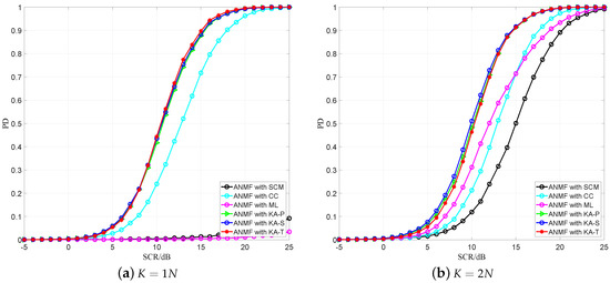
Figure 7.
PD versa SCR for IPIX Radar data under different number of secondary data.
According to the simulation results and IPIX radar sensor system data, we can summarize that the KA-T estimator has the best performance both in estimation and detection under the choosen condition, followed by the KA-S and KA-P estimator. Compared with the existing KA methods, i.e., the CC and ML estimator, the proposed estimators can perform better, especially in the compound-Gaussian clutter.
In addition, according to the Section 3, each structure has special application scene and some papers [58,59] have proposed methods to recognize the structure property of the covariance to help using the structure information.
5. Conclusions and Future Work
In this paper, we have considered the problem of covariance estimation with insufficient secondary data in compound-Gaussian clutter. We have proposed three knowledge-aided covariance estimators and applied the estimators to radar sensor signal detection.
According to the experimental results using simulated and measured sensor data, the KA-T estimator has the best performance both in estimation and detection, followed by the KA-S and KA-P estimator. Compared with the existing KA methods, i.e., the CC and ML estimators, the proposed estimators can perform better, especially with compound-Gaussian clutter.
Possible future research tracks might concern the design of the knowledge-aided covariance estimator based on other geometric means, such as Log–Euclidean mean, Root–Euclidean mean, Powe–Euclidean mean, and Cholesky mean.
Author Contributions
N.K. put forward the original ideas and performed the research. Z.S. conceived and designed the simulations. Q.D. reviewed the paper and provided useful comments.
Funding
This work was supported in part by the National Nature Science Foundation of China under contract numbers 61501505.
Conflicts of Interest
The authors declare no conflict of interest.
Appendix A
The detail formula derivation of is obtained in this Appendix. Equation (9) be recasted as.
According to (A1), we obtain
Then we take derivative of (A2) with respect to and nulling the result we obtain
It is noted that is unknown, but according to [23] can be replaced by in practice, namely
References
- Ward, J. Space–Time Adaptive Processing for Airborne Radar; Technical Report; MIT Press: Cambridge, MA, USA, 1994. [Google Scholar]
- Kelly, E.J. An Adaptive Detection Algorithm. IEEE Trans. Aerosp. Electron. Syst. 1986, AES-22, 115–127. [Google Scholar] [CrossRef]
- Liu, W.; Xie, W.; Liu, J.; Wang, Y. Adaptive Double Subspace Signal Detection in Gaussian Background Part I: Homogeneous Environments. IEEE Trans. Signal Process. 2014, 62, 2345–2357. [Google Scholar] [CrossRef]
- Liu, W.; Xie, W.; Liu, J.; Wang, Y. Adaptive Double Subspace Signal Detection in Gaussian Background Part II: Partially Homogeneous Environments. IEEE Trans. Signal Process. 2014, 62, 2358–2369. [Google Scholar] [CrossRef]
- Shang, Z.; Du, Q.; Tang, Z.; Zhang, T.; Liu, W. Multichannel adaptive signal detection in structural nonhomogeneous environment characterized by the generalized eigenrelation. Signal Process. 2018, 148, 214–222. [Google Scholar] [CrossRef]
- Liu, J.; Zhou, S.; Liu, W.; Zheng, J.; Liu, H.; Li, J. Tunable Adaptive Detection in Colocated MIMO Radar. IEEE Trans. Signal Process. 2018, 66, 1080–1092. [Google Scholar] [CrossRef]
- Goodman, N.R. Statistical analysis based on a certain multivariate complex Gaussian distribution (an introduction). Ann. Math. Stat. 1963, 34, 152–177. [Google Scholar] [CrossRef]
- Gini, F.; Rangaswamy, M. Knowledge Based Radar Detection, Tracking and Classification (Adaptive and Learning Systems for Signal Processing, Communications and Control Series); Wiley: Hoboken, NJ, USA, 2008. [Google Scholar]
- Conte, E.; Lops, M.; Ricci, G. Adaptive matched filter detection in spherically invariant noise. IEEE Signal Process. Lett. 1996, 3, 248–250. [Google Scholar] [CrossRef]
- Pascal, F.; Chitour, Y.; Ovarlez, J.P.; Forster, P.; Larzabal, P. Covariance Structure Maximum-Likelihood Estimates in Compound Gaussian Noise: Existence and Algorithm Analysis. IEEE Trans. Signal Process. 2008, 56, 34–48. [Google Scholar] [CrossRef]
- Gini, F.; Greco, M. Covariance matrix estimation for CFAR Detection in correlated heavy tailed clutter. Signal Process. 2002, 82, 1847–1859. [Google Scholar] [CrossRef]
- Dai, B.; Wang, T.; Wu, J.; Bao, Z. Adaptively iterative weighting covariance matrix estimation for airborne radar clutter suppression. Signal Process. 2015, 106, 282–293. [Google Scholar] [CrossRef]
- Aubry, A.; Maio, A.D.; Pallotta, L.; Farina, A. Covariance matrix estimation via geometric barycenters and its application to radar training data selection. IET Radar Sonar Navig. 2013, 7, 600–614. [Google Scholar] [CrossRef]
- Cui, G.; Li, N.; Pallotta, L.; Foglia, G.; Kong, L. Geometric barycenters for covariance estimation in compound-Gaussian clutter. IET Radar Sonar Navig. 2017, 11, 404–409. [Google Scholar] [CrossRef]
- Hua, X.; Cheng, Y.; Wang, H.; Qin, Y.; Li, Y. Geometric means and medians with applications to target detection. IET Signal Process. 2017, 11, 711–720. [Google Scholar] [CrossRef]
- Brennan, L.E.; Reed, I.S. Theory of Adaptive Radar. IEEE Trans. Aerosp. Electron. Syst. 1973, AES-9, 237–252. [Google Scholar] [CrossRef]
- Guerci, J.R.; Baranoski, E.J. Knowledge-aided adaptive radar at DARPA: An overview. IEEE Signal Process. Mag. 2006, 23, 41–50. [Google Scholar] [CrossRef]
- Haykin, S. Cognitive radar: A way of the future. IEEE Signal Process. Mag. 2006, 23, 30–40. [Google Scholar] [CrossRef]
- Conte, E.; Maio, A.D.; Farina, A.; Foglia, G. Design and analysis of a knowledge-aided radar detector for doppler processing. IEEE Trans. Aerosp. Electron. Syst. 2006, 42, 1058–1079. [Google Scholar] [CrossRef]
- Foglia, G.; Hao, C.; Giunta, G.; Orlando, D. Knowledge-aided adaptive detection in partially homogeneous clutter: Joint exploitation of persymmetry and symmetric spectrum. Digit. Signal Process. 2017, 67, 131–138. [Google Scholar] [CrossRef]
- Foglia, G.; Hao, C.; Farina, A.; Giunta, G.; Orlando, D.; Hou, C. Adaptive Detection in Partially Homogeneous Clutter with Symmetric Spectrum. IEEE Trans. Aerosp. Electron. Syst. 2017, 54, 2110–2119. [Google Scholar] [CrossRef]
- Pailloux, G.; Forster, P.; Ovarlez, J.P.; Pascal, F. Persymmetric Adaptive Radar Detectors. IEEE Trans. Aerosp. Electron. Syst. 2011, 47, 2376–2390. [Google Scholar] [CrossRef]
- Stoica, P.; Li, J.; Zhu, X.; Guerci, J.R. On Using a priori Knowledge in space–Time Adaptive Processing. IEEE Trans. Signal Process. 2008, 56, 2598–2602. [Google Scholar] [CrossRef]
- Zhu, X.; Li, J.; Stoica, P. Knowledge-Aided space–Time Adaptive Processing. IEEE Trans. Aerosp. Electron. Syst. 2011, 47, 1325–1336. [Google Scholar] [CrossRef]
- Maio, A.D.; Foglia, G.; Farina, A.; Piezzo, M. Estimation of the covariance matrix based on multiple a-priori models. In Proceedings of the IEEE Radar Conference, Arlington, VA, USA, 10–14 May 2010; pp. 1025–1029. [Google Scholar]
- Wu, Y.; Tang, J.; Peng, Y. On the Essence of Knowledge-Aided Clutter Covariance Estimate and Its Convergence. IEEE Trans. Aerosp. Electron. Syst. 2011, 47, 569–585. [Google Scholar] [CrossRef]
- Hao, C.; Orlando, D.; Foglia, G.; Giunta, G. Knowledge-Based Adaptive Detection: Joint Exploitation of Clutter and System Symmetry Properties. IEEE Signal Process. Lett. 2016, 23, 1489–1493. [Google Scholar] [CrossRef]
- Cai, L.; Wang, H. A persymmetric multiband GLR algorithm. IEEE Trans. Aerosp. Electron. Syst. 1992, 28, 806–816. [Google Scholar] [CrossRef]
- Chen, Y.; Wiesel, A.; Eldar, Y.C.; Hero, A.O. Shrinkage Algorithms for MMSE Covariance Estimation. IEEE Trans. Signal Process. 2010, 58, 5016–5029. [Google Scholar] [CrossRef]
- Pascal, F.; Chitour, Y.; Quek, Y. Generalized Robust Shrinkage Estimator and Its Application to STAP Detection Problem. IEEE Trans. Signal Process. 2014, 62, 5640–5651. [Google Scholar] [CrossRef]
- Riedl, M.; Potter, L.C. Multimodel Shrinkage for Knowledge-Aided space–Time Adaptive Processing. IEEE Trans. Aerosp. Electron. Syst. 2018, 54, 2601–2610. [Google Scholar] [CrossRef]
- Besson, O.; Tourneret, J.Y.; Bidon, S. Knowledge-Aided Bayesian Detection in Heterogeneous Environments. IEEE Signal Process. Lett. 2007, 14, 355–358. [Google Scholar] [CrossRef]
- Bidon, S.; Besson, O.; Tourneret, J.Y. A Bayesian Approach to Adaptive Detection in Nonhomogeneous Environments. IEEE Trans. Signal Process. 2008, 56, 205–217. [Google Scholar] [CrossRef]
- Bandiera, F.; Besson, O.; Ricci, G. Knowledge-aided covariance matrix estimation and adaptive detection in compound-Gaussian noise. IEEE Trans. Signal Process. 2010, 58, 5391–5396. [Google Scholar] [CrossRef]
- Gurram, P.R.; Goodman, N.A. Spectral-domain covariance estimation with a priori knowledge. IEEE Trans. Aerosp. Electron. Syst. 2006, 42, 1010–1020. [Google Scholar] [CrossRef]
- Techau, P.M.; Guerci, J.R.; Slocumb, T.H.; Griffiths, L.J. Performance bounds for hot and cold clutter mitigation. IEEE Trans. Aerosp. Electron. Syst. 1999, 35, 1253–1265. [Google Scholar] [CrossRef]
- Capraro, C.T.; Capraro, G.T.; Maio, A.D.; Farina, A.; Wicks, M. Demonstration of knowledge-aided space–time adaptive processing using measured airborne data. IEE Proc. Radar Sonar Navig. 2007, 153, 487–494. [Google Scholar] [CrossRef]
- De Maio, A.; Foglia, G.; Conte, E.; Farina, A. CFAR behavior of adaptive detectors: An experimental analysis. IEEE Trans. Aerosp. Electron. Syst. 2005, 41, 233–251. [Google Scholar] [CrossRef]
- Bidon, S.; Besson, O.; Tourneret, J.Y. Knowledge-Aided STAP in Heterogeneous Clutter using a Hierarchical Bayesian Algorithm. IEEE Trans. Aerosp. Electron. Syst. 2011, 47, 1863–1879. [Google Scholar] [CrossRef]
- Fortunati, S.; Gini, F.; Greco, M.S. The Misspecified Cramer-Rao Bound and Its Application to Scatter Matrix Estimation in Complex Elliptically Symmetric Distributions. IEEE Trans. Signal Process. 2016, 64, 2387–2399. [Google Scholar] [CrossRef]
- Fortunati, S.; Gini, F.; Greco, M.S.; Richmond, C.D. Performance Bounds for Parameter Estimation under Misspecified Models: Fundamental Findings and Applications. IEEE Signal Process. Mag. 2017, 34, 142–157. [Google Scholar] [CrossRef]
- Fortunati, S.; Gini, F.; Greco, M.S. The Constrained Misspecified Cramér-Rao Bound. IEEE Signal Process. Lett. 2016, 23, 718–721. [Google Scholar] [CrossRef]
- Maio, A.D.; Farina, A.; Foglia, G. Knowledge-Aided Bayesian Radar Detectors and Their Application to Live Data. IEEE Trans. Aerosp. Electron. Syst. 2010, 46, 170–183. [Google Scholar] [CrossRef]
- Wang, P.; Li, H.; Besson, O.; Fang, J. Knowledge-aided hyperparameter-free Bayesian detection in stochastic homogeneous environments. In Proceedings of the IEEE International Conference on Acoustics, Speech and Signal Processing, Shanghai, China, 20–25 March 2016; pp. 2901–2905. [Google Scholar]
- Gao, Y.; Li, H.; Himed, B. Knowledge-Aided Range-Spread Target Detection for Distributed MIMO Radar in Non-Homogeneous Environments. IEEE Trans. Signal Process. 2017, 65, 617–627. [Google Scholar] [CrossRef]
- Sangston, K.J.; Gini, F.; Greco, M.V.; Farina, A. Structures for radar detection in compound Gaussian clutter. IEEE Trans. Aerosp. Electron. Syst. 1999, 35, 445–458. [Google Scholar] [CrossRef]
- Sangston, K.J.; Gini, F.; Greco, M.S. Coherent Radar Target Detection in Heavy-Tailed Compound-Gaussian Clutter. IEEE Trans. Aerosp. Electron. Syst. 2012, 48, 64–77. [Google Scholar] [CrossRef]
- Pennec, X. Intrinsic Statistics on Riemannian Manifolds: Basic Tools for Geometric Measurements. J. Math. Imaging Vis. 2006, 25, 127–154. [Google Scholar] [CrossRef]
- Nitzberg, R. Application of Maximum Likelihood Estimation of Persymmetric Covariance Matrices to Adaptive Processing. IEEE Trans. Aerosp. Electron. Syst. 1980, AES-16, 124–127. [Google Scholar] [CrossRef]
- Fuhrmann, D.R. Application of Toeplitz covariance estimation to adaptive beamforming and detection. IEEE Trans. Signal Process. 1991, 39, 2194–2198. [Google Scholar] [CrossRef]
- Kraut, S.; Scharf, L.L. The CFAR adaptive subspace detector is a scale-invariant GLRT. IEEE Trans. Signal Process. Publ. IEEE Signal Process. Soc. 1999, 47, 2538–2541. [Google Scholar] [CrossRef]
- Gini, F.; Greco, M.V. Suboptimum approach to adaptive coherent radar detection in compound-Gaussian clutter. IEEE Trans. Aerosp. Electron. Syst. 1999, 35, 1095–1104. [Google Scholar] [CrossRef]
- Balleri, A.; Nehorai, A.; Wang, J. Maximum likelihood estimation for compound-gaussian clutter with inverse gamma texture. IEEE Trans. Aerosp. Electron. Syst. 2007, 43, 775–779. [Google Scholar] [CrossRef]
- Farina, A.; Gini, F.; Greco, M.V.; Verrazzani, L. High resolution sea clutter data: Statistical analysis of recorded live data. IEEE Proc. Radar Sonar Navig. 1997, 144, 121–130. [Google Scholar] [CrossRef]
- Gini, F.; Greco, M.V.; Diani, M.; Verrazzani, L. Performance analysis of two adaptive radar detectors against non-Gaussian real sea clutter data. IEEE Trans. Aerosp. Electron. Syst. 2000, 36, 1429–1439. [Google Scholar]
- Conte, E.; De Maio, A.; Galdi, C. Statistical analysis of real clutter at different range resolutions. IEEE Trans. Aerosp. Electron. Syst. 2004, 40, 903–918. [Google Scholar] [CrossRef]
- Wang, P.; Sahinoglu, Z.; Pun, M.O.; Li, H.; Himed, B. Knowledge-Aided Adaptive Coherence Estimator in Stochastic Partially Homogeneous Environments. IEEE Signal Process. Lett. 2011, 18, 193–196. [Google Scholar] [CrossRef]
- Carotenuto, V.; Maio, A.D.; Orlando, D.; Stoica, P. Model Order Selection Rules for Covariance Structure Classification in Radar. IEEE Trans. Signal Process. 2017, 65, 5305–5317. [Google Scholar] [CrossRef]
- Carotenuto, V.; Maio, A.D.; Orlando, D.; Stoica, P. Radar Detection Architecture based on Interference Covariance Structure Classification. IEEE Trans. Aerosp. Electron. Syst. 2018. [Google Scholar] [CrossRef]
© 2019 by the authors. Licensee MDPI, Basel, Switzerland. This article is an open access article distributed under the terms and conditions of the Creative Commons Attribution (CC BY) license (http://creativecommons.org/licenses/by/4.0/).