Robust Vehicle Detection and Counting Algorithm Employing a Convolution Neural Network and Optical Flow

 ,
, 
Abstract
1. Introduction
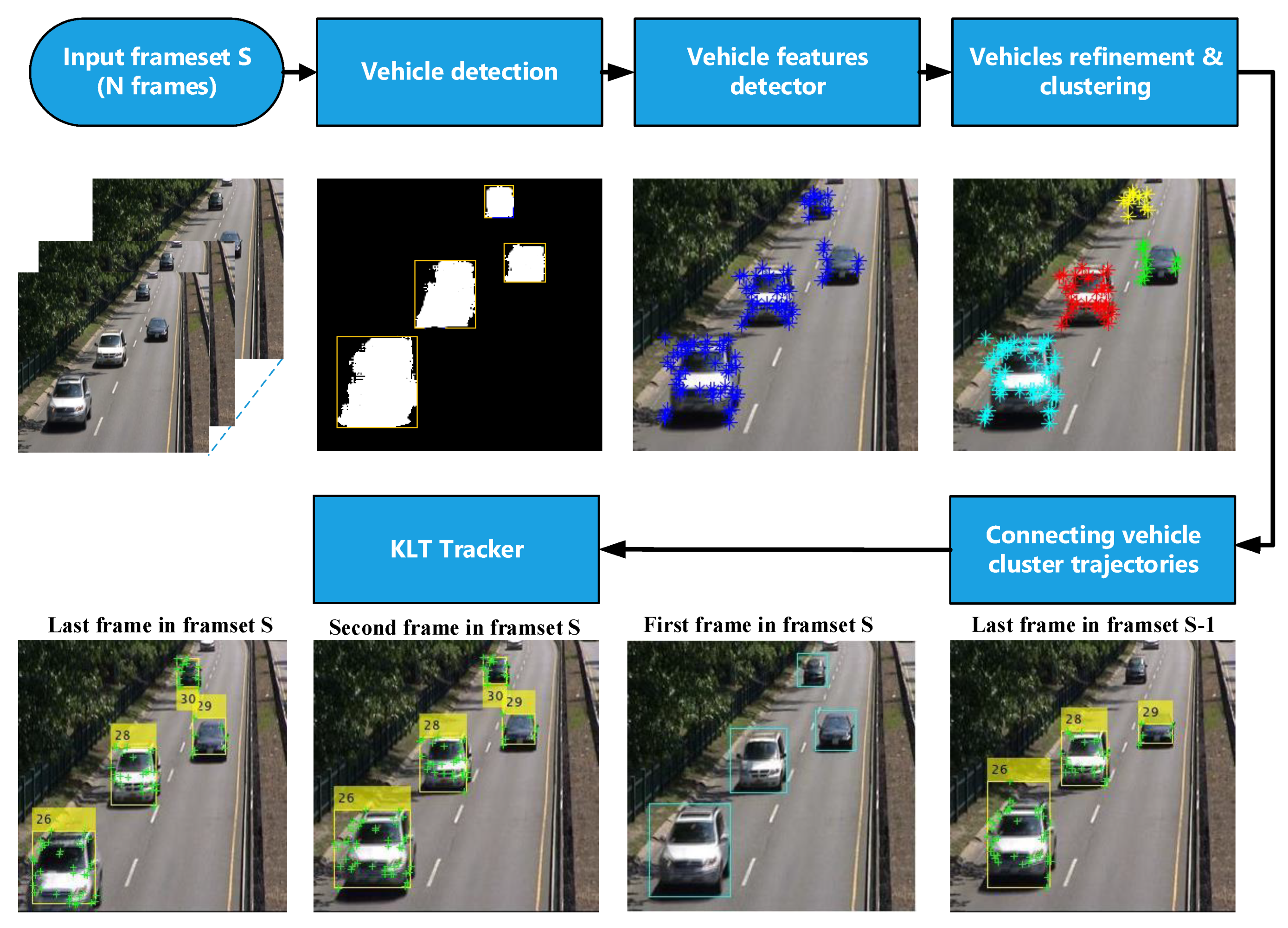
2. Methodology
2.1. Vehicle Detection
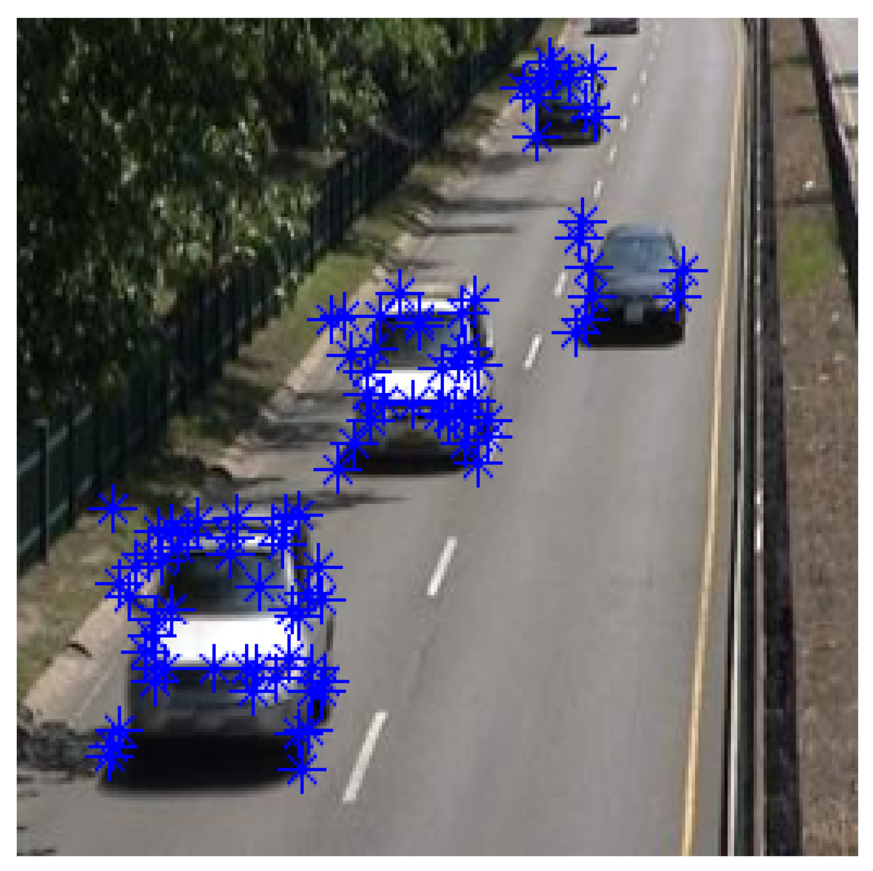
2.2. Feature Points Detector
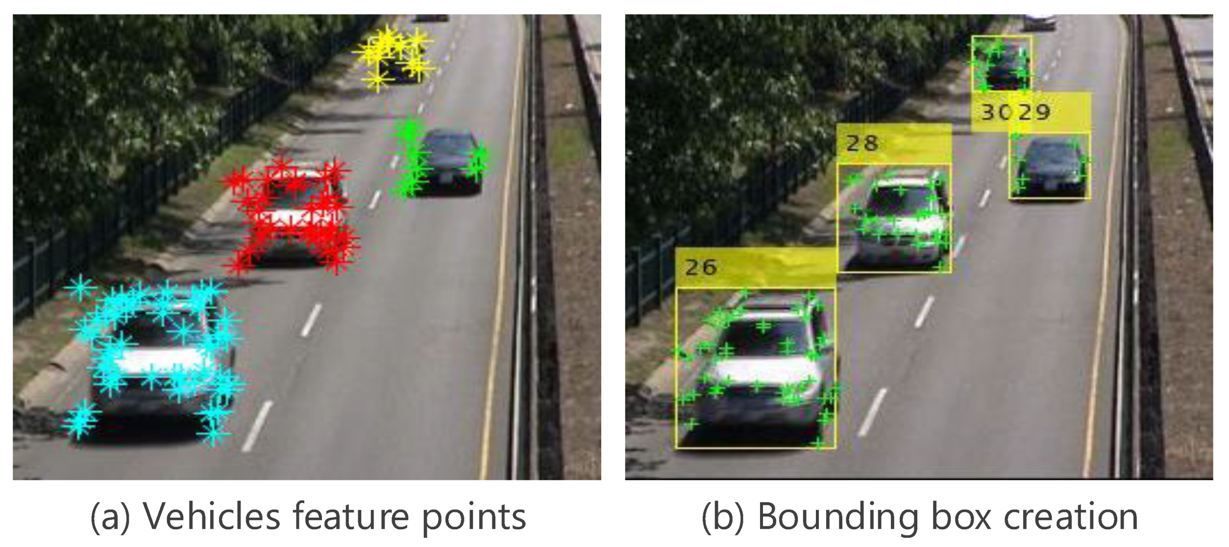
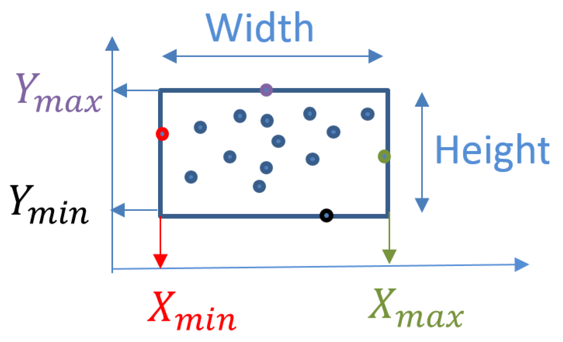
2.3. Vehicles Refinement and Clustering
K-Means Clustering
- Determine the centroid coordinates.
- Determine the distance between the centroids and each data feature.
- Group the data based on the minimum distance to find the closest centroid.
2.4. Connecting Vehicle Cluster Trajectories
3. Experimental Results
4. Conclusions
Author Contributions
Acknowledgments
Conflicts of Interest
References
- Yang, Z.; Pun-Cheng, L.S. Vehicle detection in intelligent transportation systems and its applications under varying environments: A review. Image Vis. Comput. 2018, 69, 143–154. [Google Scholar] [CrossRef]
- Lou, L.; Zhang, J.; Xiong, Y.; Jin, Y. A Novel Vehicle Detection Method Based on the Fusion of Radio Received Signal Strength and Geomagnetism. Sensors 2019, 19, 58. [Google Scholar] [CrossRef] [PubMed]
- Wang, Y.; Yu, Z.; Zhu, L. Foreground detection with deeply learned multi-scale spatial-temporal features. Sensors 2018, 18, 4269. [Google Scholar] [CrossRef] [PubMed]
- Yu, T.; Yang, J.; Lu, W. Refinement of Background-Subtraction Methods Based on Convolutional Neural Network Features for Dynamic Background. Algorithms 2019, 12, 128. [Google Scholar] [CrossRef]
- Unzueta, L.; Nieto, M.; Cortés, A.; Barandiaran, J.; Otaegui, O.; Sánchez, P. Adaptive multicue background subtraction for robust vehicle counting and classification. IEEE Trans. Intell. Transp. Syst. 2011, 13, 527–540. [Google Scholar] [CrossRef]
- Jia, Y.; Zhang, C. Front-view vehicle detection by Markov chain Monte Carlo method. Pattern Recognit. 2009, 42, 313–321. [Google Scholar] [CrossRef]
- Tsai, L.W.; Hsieh, J.W.; Fan, K.C. Vehicle detection using normalized color and edge map. IEEE Trans. Image Process. 2007, 16, 850–864. [Google Scholar] [CrossRef] [PubMed]
- Chen, J.; Xu, W.; Peng, W.; Bu, W.; Xing, B.; Liu, G. Road Object Detection Using a Disparity-Based Fusion Model. IEEE Access 2018, 6, 19654–19663. [Google Scholar] [CrossRef]
- Stauffer, C.; Grimson, W.E.L. Adaptive background mixture models for real-time tracking. In Proceedings of the 1999 IEEE Computer Society Conference on Computer Vision and Pattern Recognition (Cat. No PR00149), Fort Collins, CO, USA, 23–25 June 1999; Volume 2, pp. 246–252. [Google Scholar]
- Kamkar, S.; Safabakhsh, R. Vehicle detection, counting and classification in various conditions. IET Intell. Transp. Syst. 2016, 10, 406–413. [Google Scholar] [CrossRef]
- Maddalena, L.; Petrosino, A. Background subtraction for moving object detection in rgbd data: A survey. J. Imaging 2018, 4, 71. [Google Scholar] [CrossRef]
- Shakeri, M.; Zhang, H. COROLA: A sequential solution to moving object detection using low-rank approximation. Comput. Vis. Image Underst. 2016, 146, 27–39. [Google Scholar] [CrossRef]
- Yang, H.; Qu, S. Real-time vehicle detection and counting in complex traffic scenes using background subtraction model with low-rank decomposition. IET Intell. Transp. Syst. 2017, 12, 75–85. [Google Scholar] [CrossRef]
- Quesada, J.; Rodriguez, P. Automatic vehicle counting method based on principal component pursuit background modeling. In Proceedings of the 2016 IEEE International Conference on Image Processing (ICIP), Phoenix, AZ, USA, 25–28 September 2016; pp. 3822–3826. [Google Scholar]
- Abdelwahab, M. Fast approach for efficient vehicle counting. Electron. Lett. 2018, 55, 20–22. [Google Scholar] [CrossRef]
- Braham, M.; Van Droogenbroeck, M. Deep background subtraction with scene-specific convolutional neural networks. In Proceedings of the 2016 IEEE International Conference on Systems, Signals and Image Processing (IWSSIP), Bratislava, Slovakia, 23–25 May 2016; pp. 1–4. [Google Scholar]
- Minematsu, T.; Shimada, A.; Uchiyama, H.; Taniguchi, R.I. Analytics of deep neural network-based background subtraction. J. Imaging 2018, 4, 78. [Google Scholar] [CrossRef]
- Ke, R.; Li, Z.; Kim, S.; Ash, J.; Cui, Z.; Wang, Y. Real-time bidirectional traffic flow parameter estimation from aerial videos. IEEE Trans. Intell. Transp. Syst. 2017, 18, 890–901. [Google Scholar] [CrossRef]
- Bouguet, J.Y. Pyramidal implementation of the affine lucas kanade feature tracker description of the algorithm. Intel Corp. 2001, 5, 4. [Google Scholar]
- Kalsotra, R.; Arora, S. A Comprehensive Survey of Video Datasets for Background Subtraction. IEEE Access 2019, 7, 59143–59171. [Google Scholar] [CrossRef]
- Sheorey, S.; Keshavamurthy, S.; Yu, H.; Nguyen, H.; Taylor, C.N. Uncertainty estimation for KLT tracking. In Asian Conference on Computer Vision; Springer: Cham, Switzerland, 2014; pp. 475–487. [Google Scholar]
- Kasturi, R.; Goldgof, D.; Soundararajan, P.; Manohar, V.; Garofolo, J.; Bowers, R.; Boonstra, M.; Korzhova, V.; Zhang, J. Framework for performance evaluation of face, text, and vehicle detection and tracking in video: Data, metrics, and protocol. IEEE Trans. Pattern Anal. Mach. Intell. 2009, 31, 319–336. [Google Scholar] [CrossRef] [PubMed]
- Guerrero-Gómez-Olmedo, R.; López-Sastre, R.J.; Maldonado-Bascón, S.; Fernández-Caballero, A. Vehicle tracking by simultaneous detection and viewpoint estimation. In International Work-Conference on the Interplay Between Natural and Artificial Computation; Springer: Berlin/Heidelberg, Germany, 2013; pp. 306–316. [Google Scholar]
- Wang, Y.; Jodoin, P.M.; Porikli, F.; Konrad, J.; Benezeth, Y.; Ishwar, P. CDnet 2014: An expanded change detection benchmark dataset. In Proceedings of the 27th IEEE Conference on Computer Vision and Pattern Recognition Workshops, Columbus, OH, USA, 24–27 June 2014; pp. 387–394. [Google Scholar]


| Compared Algorithm | Advantages | Disadvantages |
|---|---|---|
| Corola [12] | Low computational complexity. Good detection result. | Only detection method. Low detection result in severe illumination changes. |
| Yang et al. [13] | Low computational complexity. Good detection and counting accuracy. Detection and Counting algorithm. | Declined counting precision accuracy. Dropping in the recall detection accuracy. |
| Quesada et al. [14] | Low computational complexity. simple counting strategy with good accuracy. | Miscounts some vehicles because of some false-positive results. Counting is based on an initial guess that leads to insufficient counting accuracy. Only counting method. |
| Mohamed [15] | Faster counting strategy. | Cannot efficiently work with different environment and weather condition. Dropping in the overall precision accuracy by using a traditional background subtraction method. Only counting method. |
| Proposed Method | Low computational complexity. Better detection and counting accuracy. Detection and counting algorithm. Working with different and complex traffic scenes. | Vehicle occlusion in specific videos influence the vehicle detection and counting. |
| Layer Type | Parameters |
|---|---|
| Input | pixels ( gray scale image patches ) |
| Convolution | 6 filters, K:, S:1 |
| Activate function | ReLU |
| Maxpooling | K:, S:3 |
| Convolution | 16 filters, K:, S:1 |
| Activate function | ReLU |
| Maxpooling | K:, S:3 |
| Fully connected | 120 hidden units |
| Sigmoid | 2 classes ( Foreground/Background ) |
| Dataset | GRAM Dataset | CDnet2014 | ATON Testbed | ||||
|---|---|---|---|---|---|---|---|
| Sequence | M-30 | M-30-HD | Highway | Intermittenpan | Streetcorneratnight | Tramstation | Highway II |
| Challenging description | Sunny day, Low resolution camera. | High resolution camera. | Sunny day, Shadows and waving trees. | Sunny day, Waving trees. | Light changes, Night scene. | Night scene, Light changes. | Crowed scene. |
| Compared Algorithm | GRAM Dataset | ATON Testbed | ||||
|---|---|---|---|---|---|---|
| M-30 | M-30-HD | Highway II | ||||
| Miss Detection | Precision | Miss Detection | Precision | Miss Detection | Precision | |
| Yang et al. [13] | 6 | 92.20 | 5 | 88.10 | 3 | 92.31 |
| Quesada et al. [14] | 2 | 97.41 | 3 | 92.86 | N/A | N/A |
| Mohamed [15] | 1 | 98.70 | 0 | 100 | 2 | 95.65 |
| Proposed Method | 0 | 100 | 0 | 100 | 1 | 97.9 |
| Method | Corola [12] | Yang et al. [13] | Proposed Method | |
|---|---|---|---|---|
| Sequence Videos | ||||
| Highway | Precission % | 95.1 | 91.3 | 98.2 |
| Recall % | 85.4 | 92.1 | 99.2 | |
| Intermittenpan | Precission % | 56.6 | 90.2 | 98.7 |
| Recall % | 58.5 | 98.8 | 97.5 | |
| Streetcorneratnight | Precission % | 82.4 | 89.1 | 95.8 |
| Recall % | 86.5 | 97.2 | 97.1 | |
| Tramstation | Precission % | 44.7 | 87.1 | 92.3 |
| Recall % | 91.0 | 97.1 | 97.1 | |
| Average accuracy | Precission % | 69.7 | 89.4 | 96.3 |
| Recall % | 80.4 | 96.3 | 97.7 | |
© 2019 by the authors. Licensee MDPI, Basel, Switzerland. This article is an open access article distributed under the terms and conditions of the Creative Commons Attribution (CC BY) license (http://creativecommons.org/licenses/by/4.0/).
Share and Cite
Gomaa, A.; Abdelwahab, M.M.; Abo-Zahhad, M.; Minematsu, T.; Taniguchi, R.-i. Robust Vehicle Detection and Counting Algorithm Employing a Convolution Neural Network and Optical Flow. Sensors 2019, 19, 4588. https://doi.org/10.3390/s19204588
Gomaa A, Abdelwahab MM, Abo-Zahhad M, Minematsu T, Taniguchi R-i. Robust Vehicle Detection and Counting Algorithm Employing a Convolution Neural Network and Optical Flow. Sensors. 2019; 19(20):4588. https://doi.org/10.3390/s19204588
Chicago/Turabian StyleGomaa, Ahmed, Moataz M. Abdelwahab, Mohammed Abo-Zahhad, Tsubasa Minematsu, and Rin-ichiro Taniguchi. 2019. "Robust Vehicle Detection and Counting Algorithm Employing a Convolution Neural Network and Optical Flow" Sensors 19, no. 20: 4588. https://doi.org/10.3390/s19204588
APA StyleGomaa, A., Abdelwahab, M. M., Abo-Zahhad, M., Minematsu, T., & Taniguchi, R.-i. (2019). Robust Vehicle Detection and Counting Algorithm Employing a Convolution Neural Network and Optical Flow. Sensors, 19(20), 4588. https://doi.org/10.3390/s19204588