Behavior-Based Control for an Aerial Robotic Swarm in Surveillance Missions


Abstract
:1. Introduction
1.1. Robotic Swarms
1.2. Aerial Swarms
1.3. Surveillance with Aerial Swarms
1.4. Contribution of This Work and General Structure
- Adaptation of the algorithm for pure surveillance with minor changes.
- Robustness analysis against communication message losses, positioning errors, and failures of the agents.
- Experiments in an indoor arena to support simulated data and demonstrate implementation.
- A realistic use of the algorithm showed by a case study.
2. Analysis of the Proposed Task
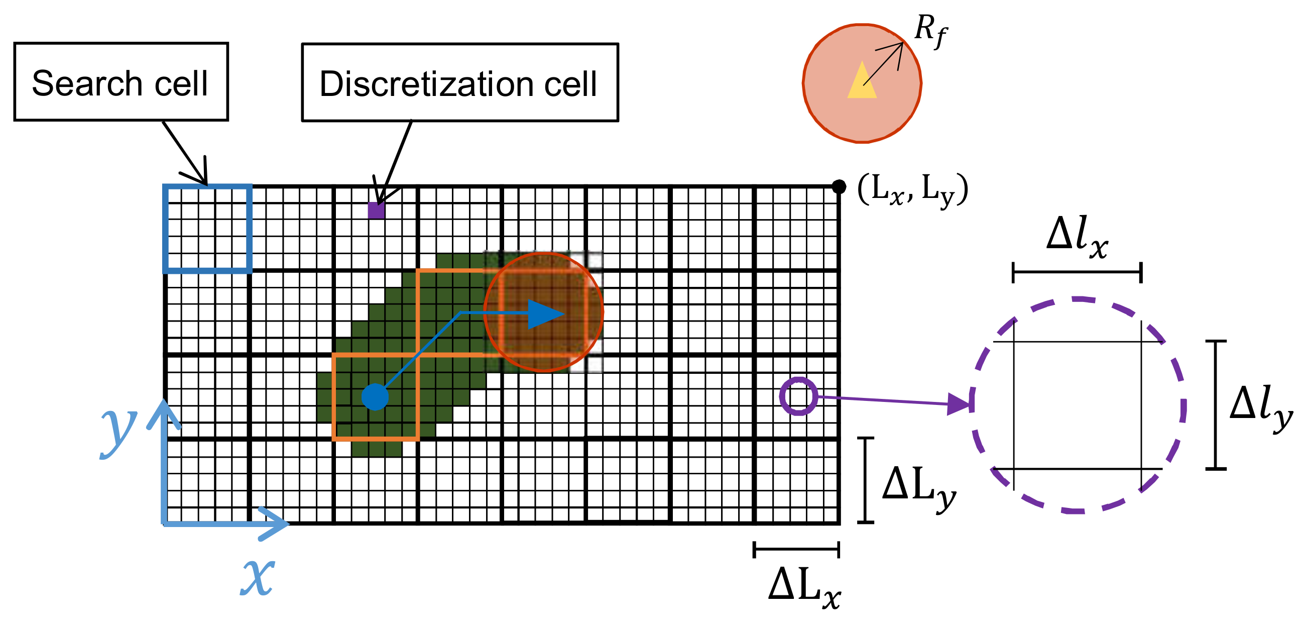
2.1. Surveillance Area
2.2. Model of the Qutadcopter
2.3. Measuring the Performance
3. Description of the Algorithm
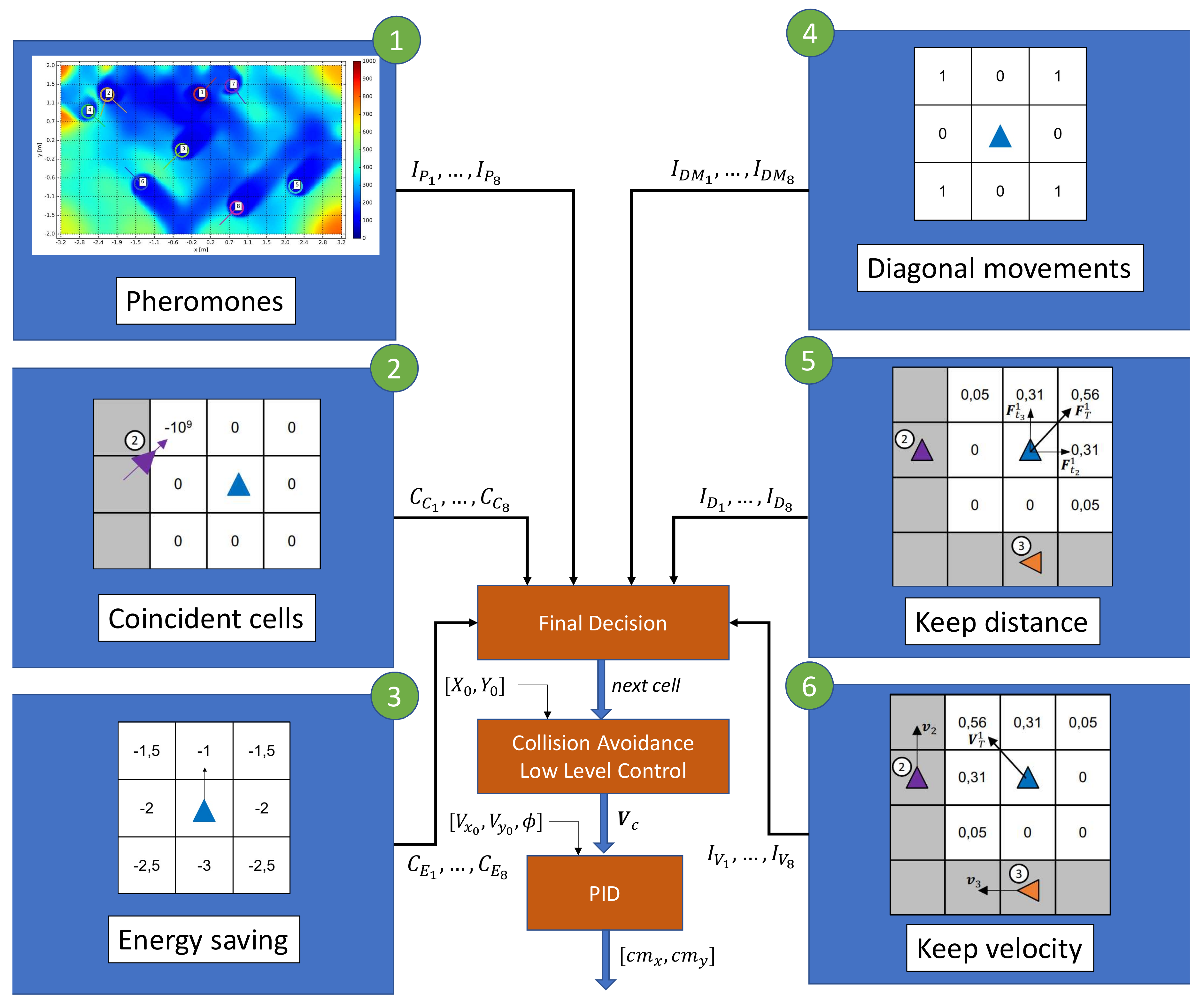
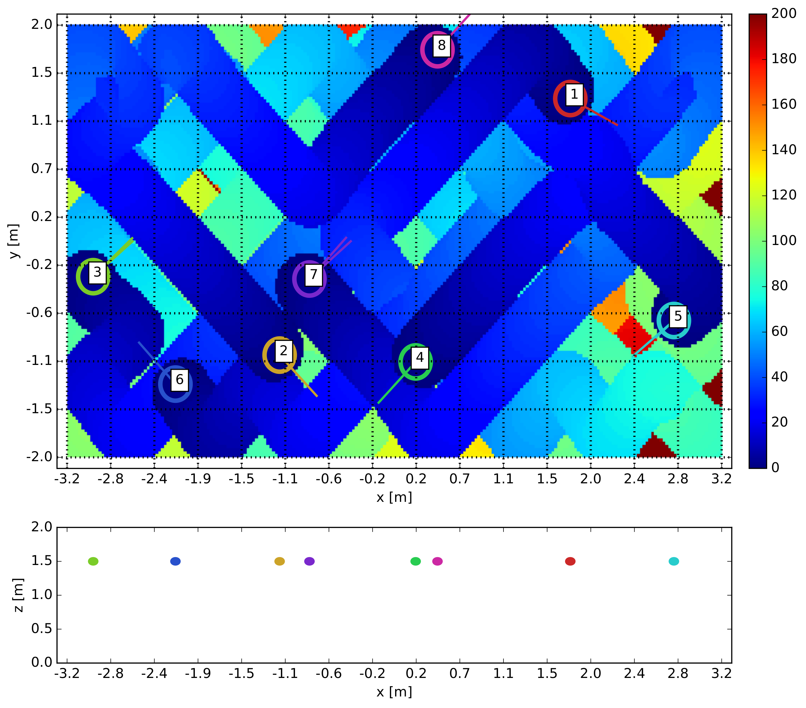
3.1. Behavior-Based Control
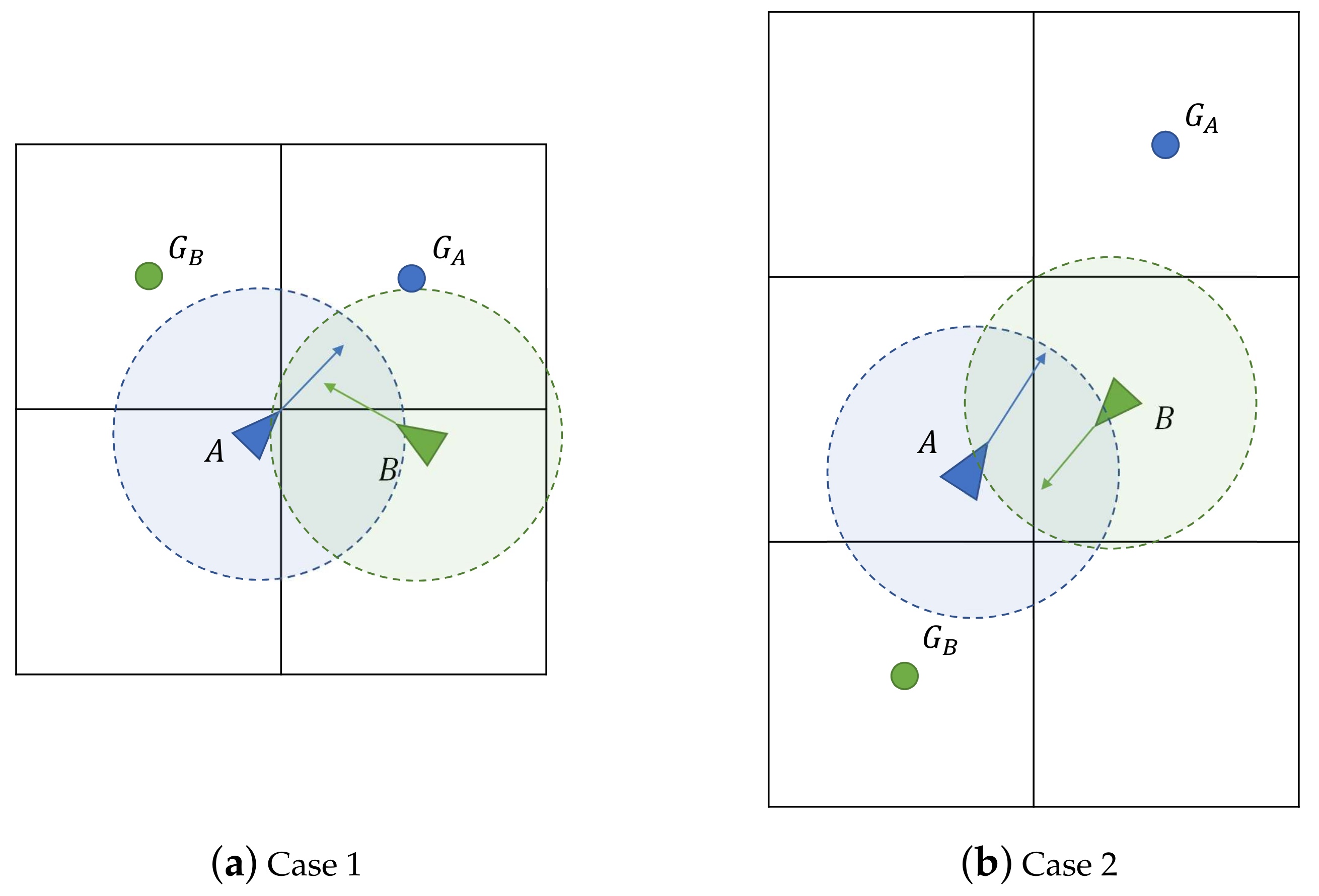
3.2. Low Level Control and Collision Avoidance
3.3. Communication Requirements
- Time stamp.
- Status information, such as taking off, landed, ready to start the mission, battery level, etc.
- Identification number of the agent, ID.
- Current position, , in global axis.
- Current velocity, , in global axis.
- Cell indexes, , to which the agent is heading to.
- Exchanged cell indexes, . If there is not currently any exchanged cell, this field is set to .
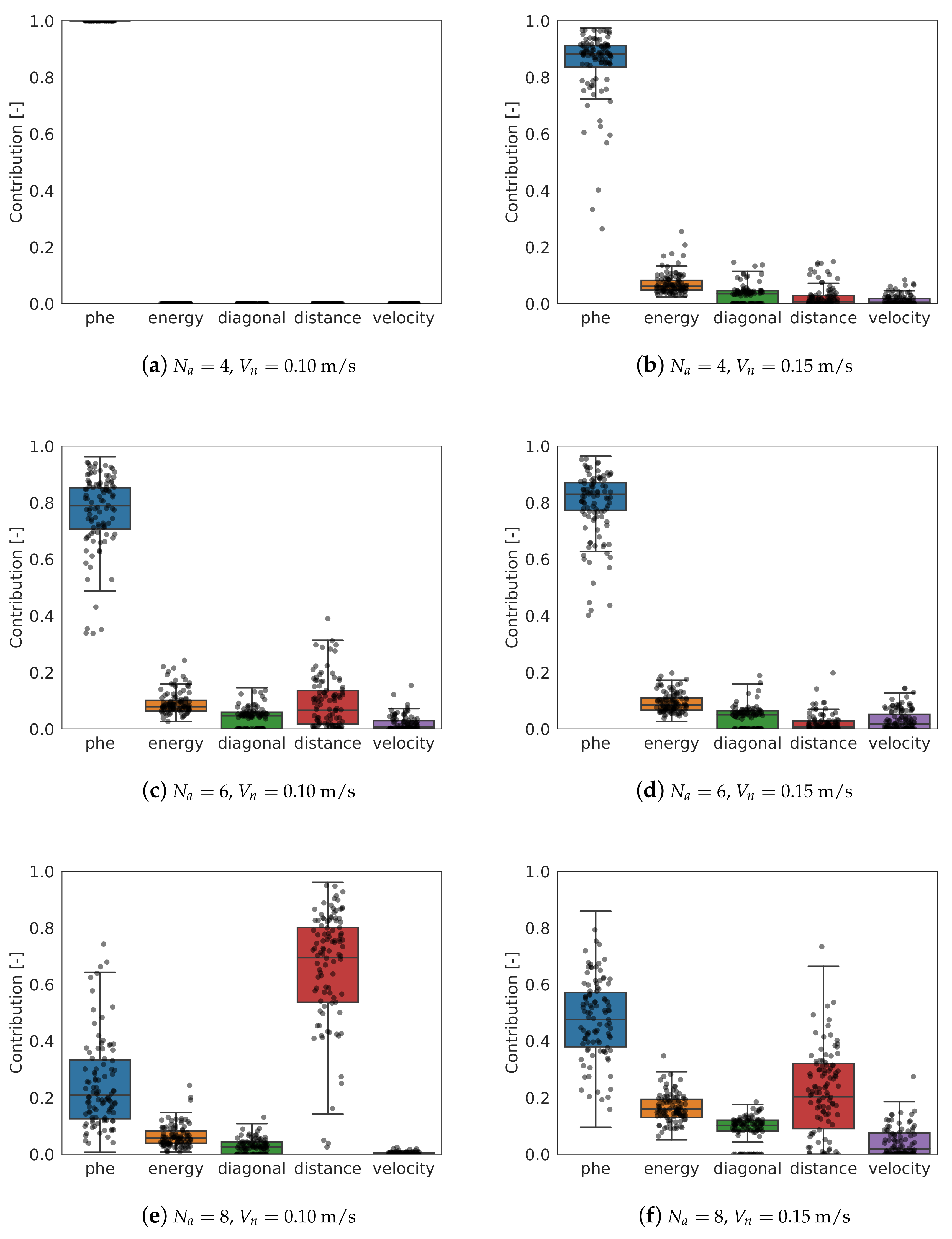
3.4. Optimization
- Chain of genes: a vector made up by the 13 parameters of the algorithm. Each of the genes is normalized with a range of valid values.
- Population: 100 members.
- Initial population: randomly generated.
- Fitness function: To evaluate each member, Equation (10) is used. The duration of the surveillance has been set to 600 s. The efficiency is averaged over 5 simulations with different initial positions.
- Crossover: 50 new members are generated. The parents are paired using the roulette-wheel technique, with a probability proportional to the efficiency value. The genes of the parents are created by applying a weighted sum of each gene individually. The weighting coefficient is a random number between 0 and 1.
- Next generation selection: the new members are evaluated and the best 100 (from the total population of 100 parents and 50 of the offspring) are selected for the next generation.
- Stopping criteria: the optimization is stopped when one of these criteria is met:
- -
- Maximum number of generations (20) has been reached.
- -
- Maximum number of generations (5) without an improvement higher than 10% of the best member has been reached.
- -
- Maximum number of generations (5) without an improvement higher than 10% of the mean efficiency of the population has been reached.
4. Simulation Results
5. Robustness Analysis
5.1. Lost of Broadcast Messages
5.2. Positioning Errors
5.3. Failure of Drones
6. Experiment Results
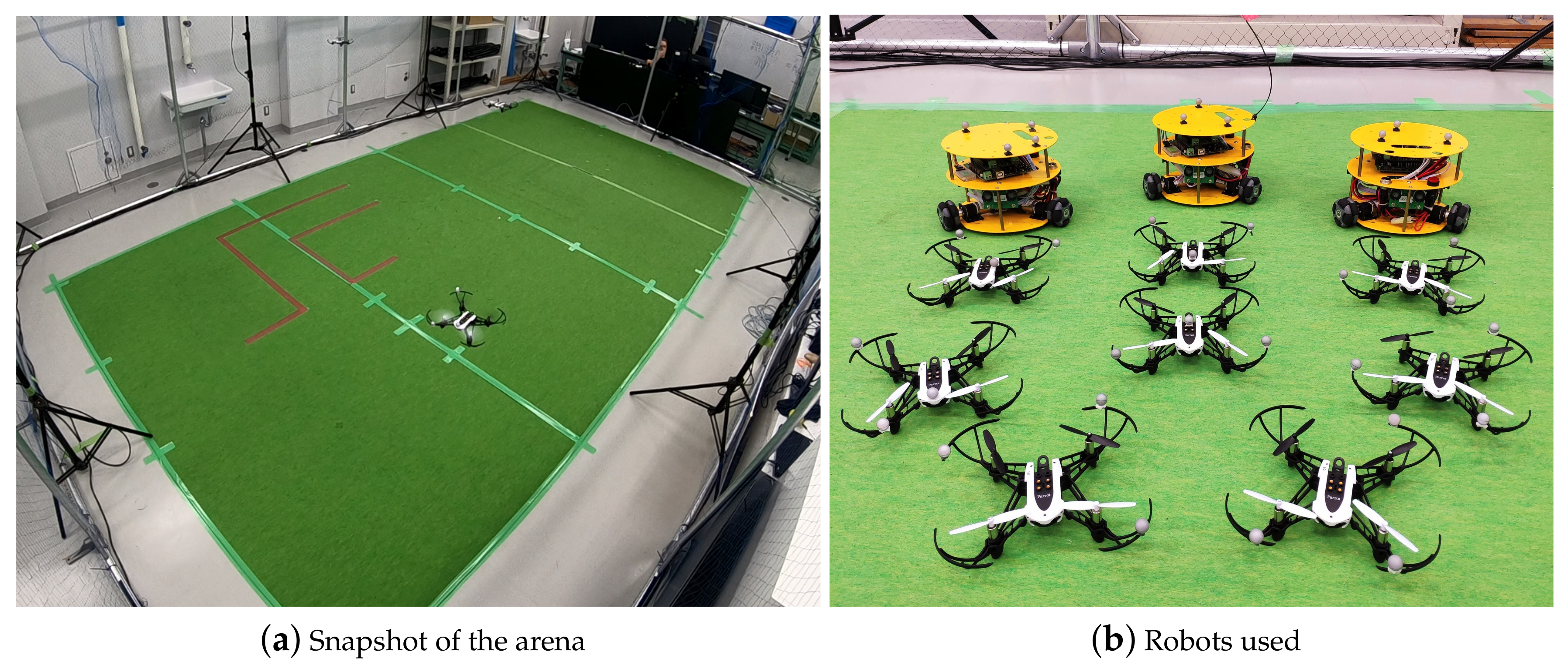
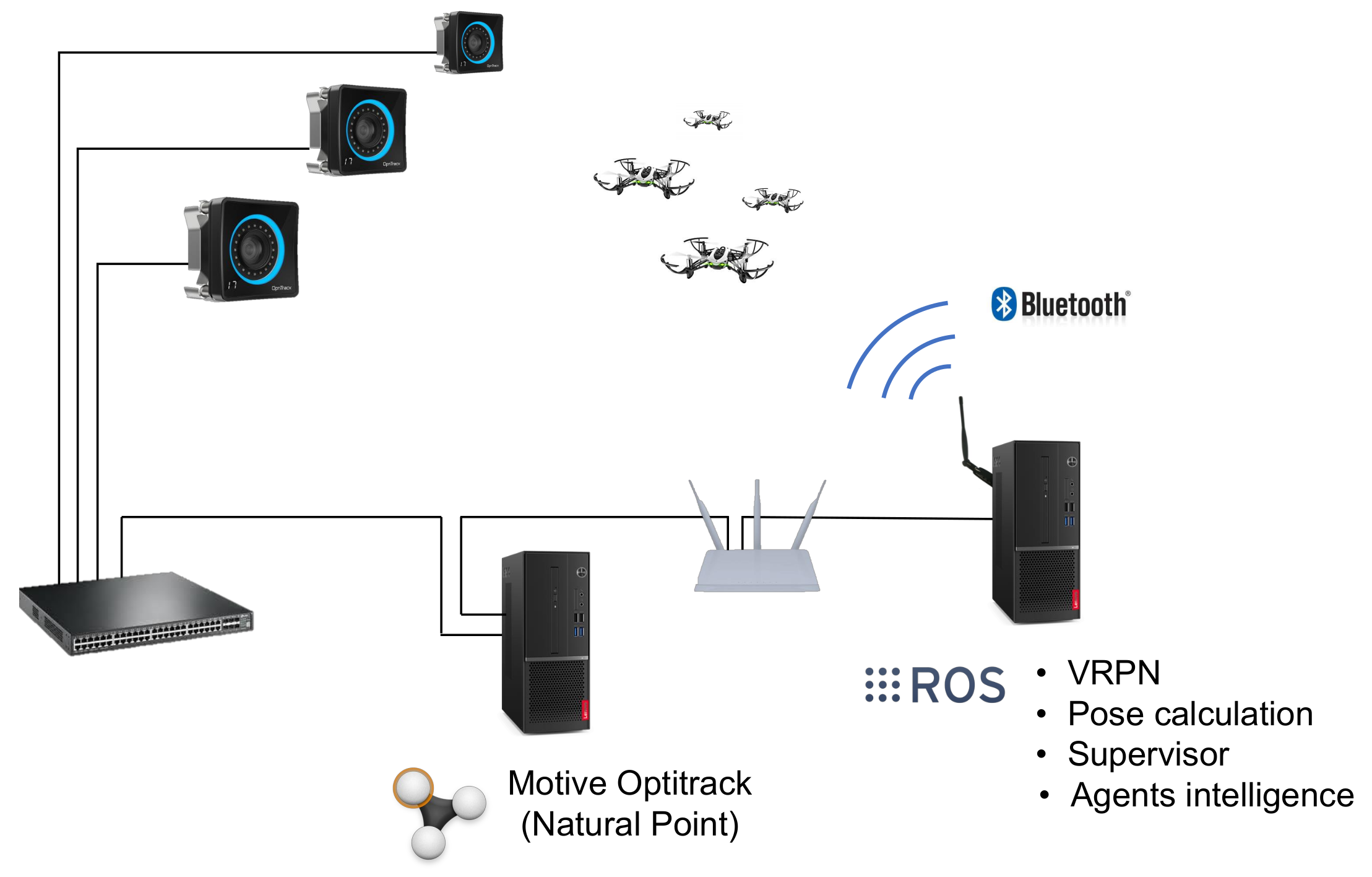
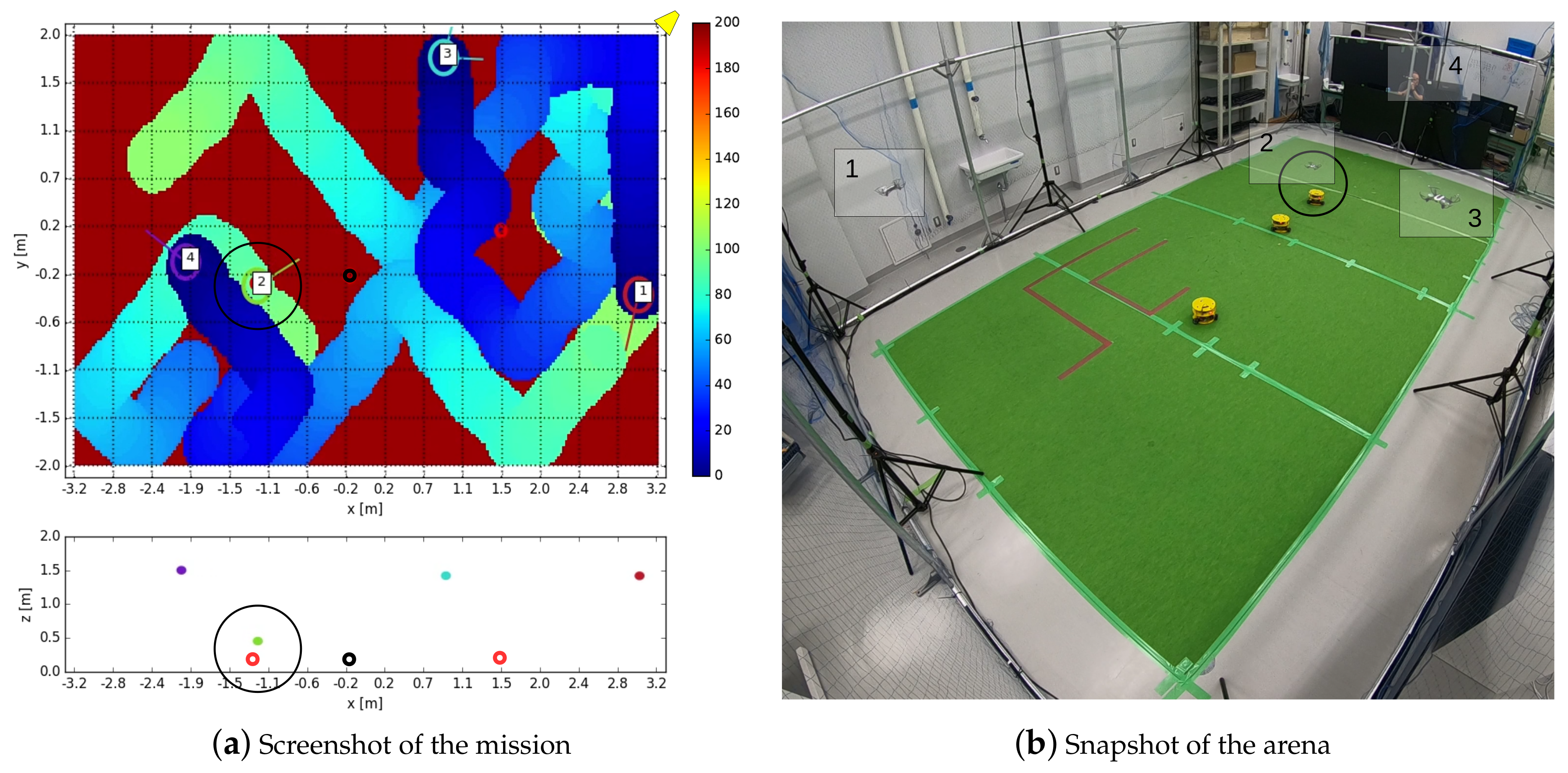
6.1. Test Arena and Drones Used
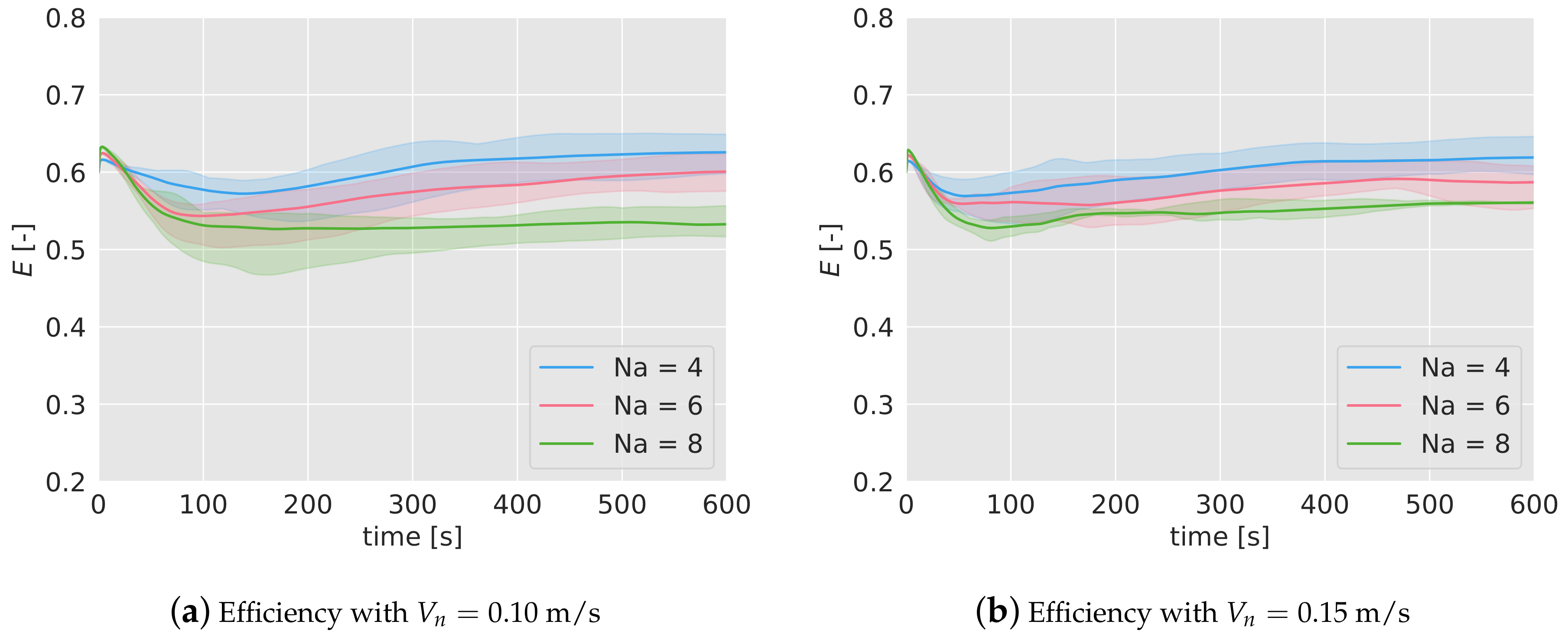
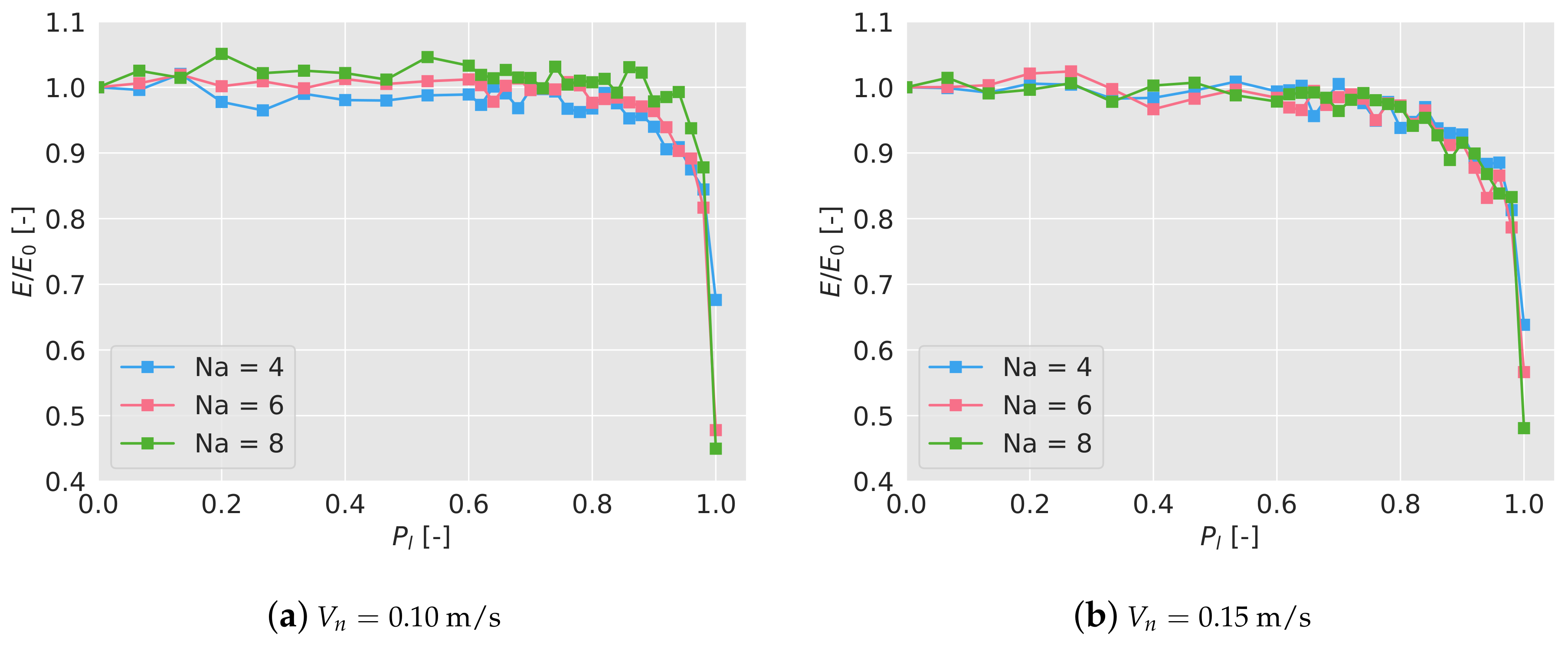
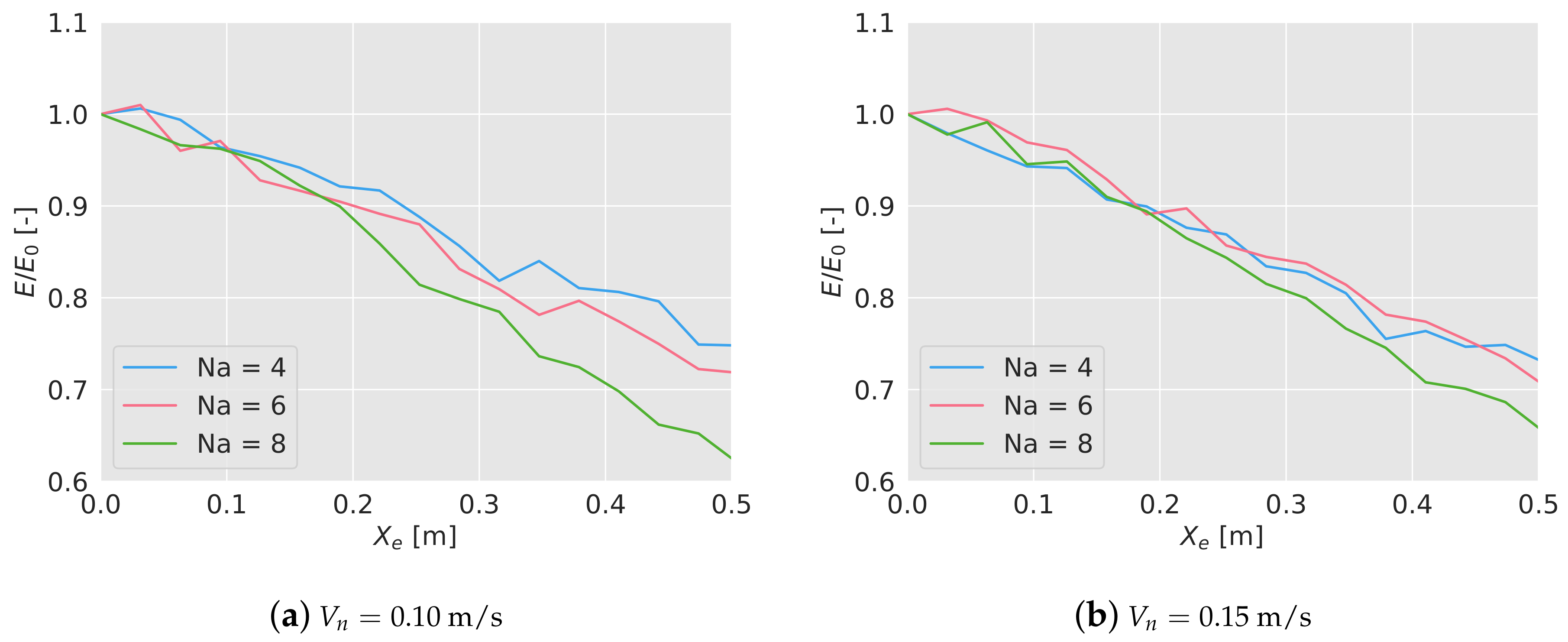
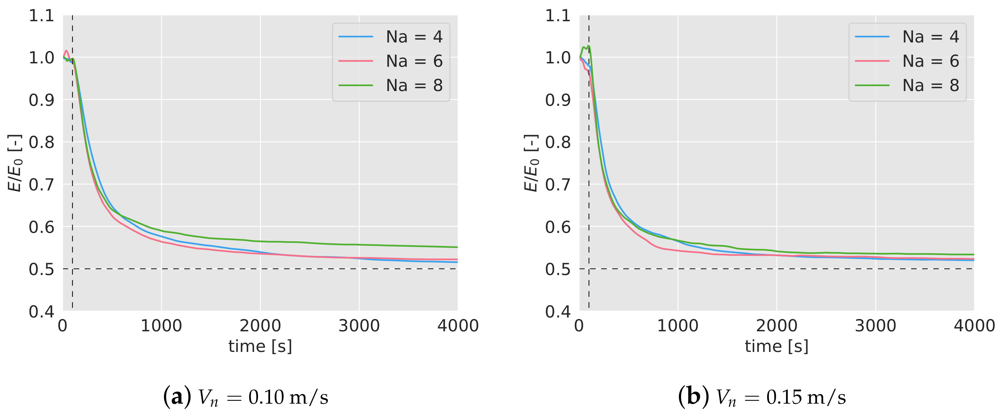
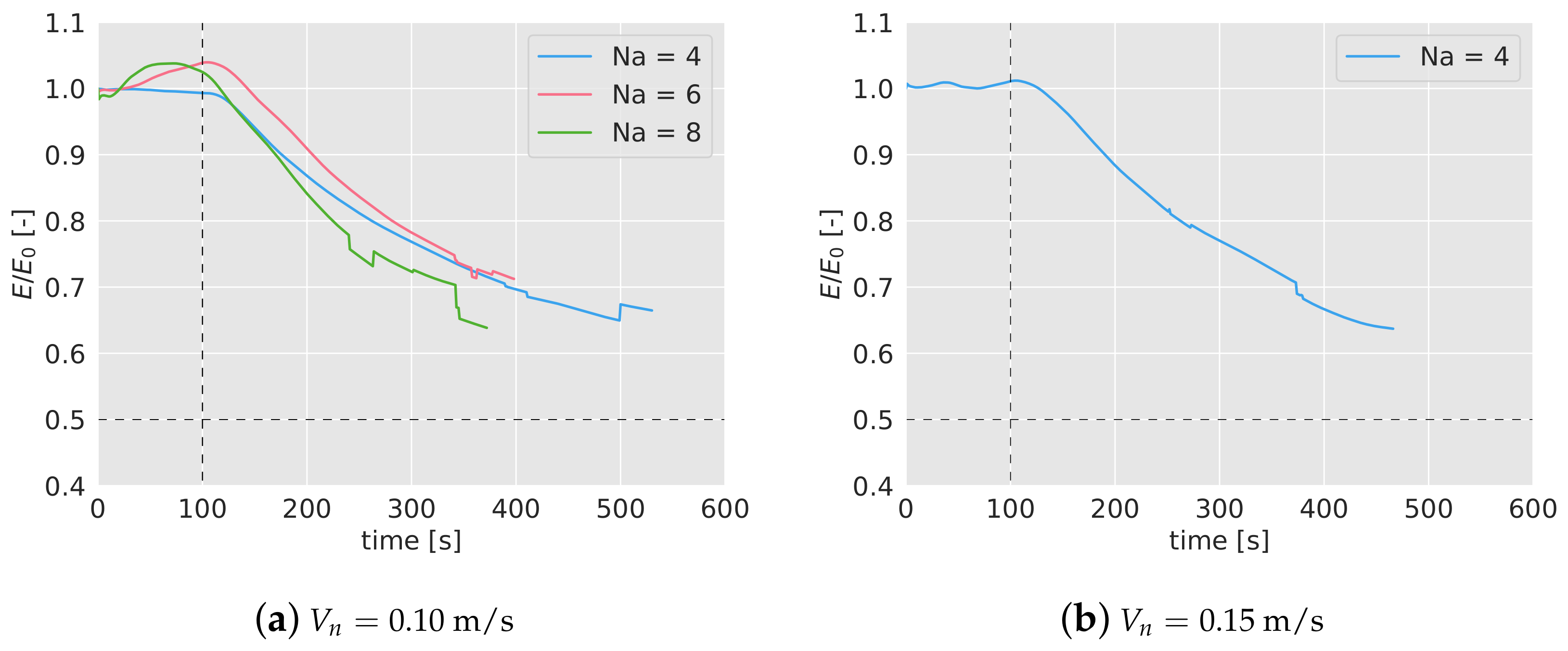
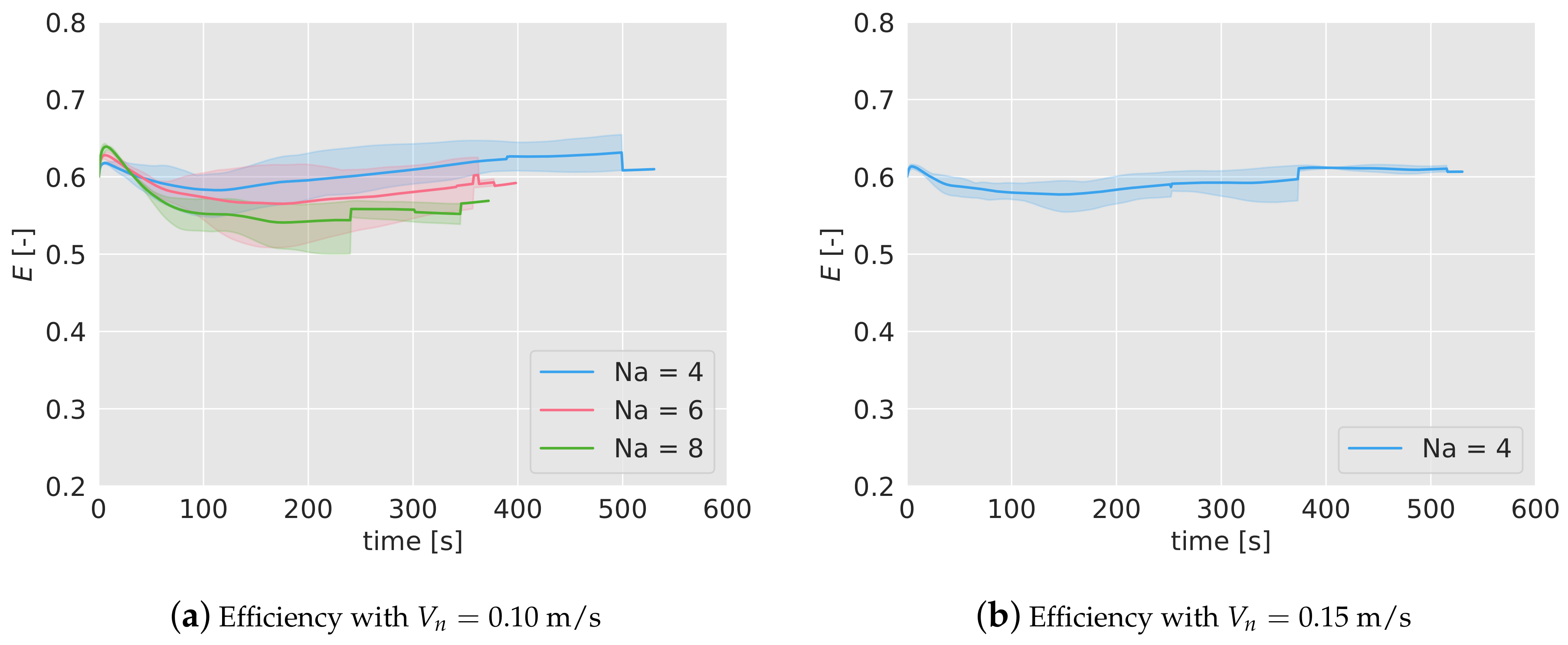
6.2. Efficiency
6.3. Failure Test
7. Case Study: Surveillance Mission with Intruders
- 4 quadcopters continuously fly over the area (6.4 × 4 m), looking for possible intruders. The flying speed is 0.10 m/s or 0.15 m/s.
- 3 robots (see Figure 10b), representing intruders, move continuously on the ground with nominal speeds between 0 and 0.10 m/s. Each ground robot generates a random point, to which they move avoiding collisions between them. When a robot reaches its destination point, it generates a new one, and moves towards it again.
- Each ground robot belongs to one of two types: friend or enemy. Each ground robot generates its type every 60 seconds with the same probability of being friend or enemy.
- When a quadcopter detects one of the robots, it reduces its altitude from 1.5 to 0.5 m to observe it. The quadcopter has the ability of discerning whether the robot is friend or enemy in 30 s. If the robot is friend, the quadcopters flies back to the nominal altitude and keeps on with the surveillance. If it is declared as enemy, the quadcopter tracks it for another 30 s.
- While an intruder is being observed, it does not change its type. When it is not being observed anymore, after 30 s, it generates another type.
8. Conclusions and Future Works
- Distributed: the algorithm can be executed on board, using the information broadcast from the other agents. Only very high level commands are needed from the central control (such as start or finish the mission).
- Robust: against losses of messages between the agents, positioning errors, and failures of some members of the team.
- Flexible: it can adapt to different scenarios (different number of agents, area size, flying speeds, etc.), keeping a high efficiency. Areas with higher interest can be included, as well as obstacles.
- Stochasticity: which may be important in some cases, given the difficulty in forecasting the agents’ movements, and making more difficult to burst into a sensitive areas without being detected.
Author Contributions
Funding
Acknowledgments
Conflicts of Interest
Appendix A

| Behavior | Param. | Description | Range | S1 | S2 | S3 | S4 | S5 | S6 |
|---|---|---|---|---|---|---|---|---|---|
| Pheromones | Init. phe. value | [0,100] | 55.2 | 50.8 | 82.0 | 56.4 | 61.5 | 58.3 | |
| S | Source of phe. | [0,5] | 3.6 | 3.0 | 3.7 | 3.5 | 4.6 | 4.3 | |
| D | Diff. coeff. | [0,0.002] | 7.5e-4 | 6.4e-4 | 4.4e-4 | 8.5e-4 | 4.7e-4 | 8.6e-4 | |
| Drop of phe. | [−1,0] | −0.72 | −0.57 | −0.62 | −0.64 | −0.78 | −0.53 | ||
| Evaluating mode | [0,1] | 0.49 | 0.57 | 0.75 | 0.66 | 0.90 | 0.60 | ||
| Keep dist. | | | [0,5] | 1.4 | 1.4 | 1.5 | 1.5 | 3.7 | 1.8 | |
| | is max. | [0,10] | 5.2 | 4.1 | 4.4 | 4.6 | 8.4 | 4.0 | ||
| Distance coeff. | [0,1] | 0.56 | 0.54 | 0.73 | 0.39 | 0.61 | 0.45 | ||
| Keep vel. | Distance coeff. | [−10,10] | 1.8 | 4.1 | 4.2 | 4.8 | 0.93 | 5.1 | |
| Final decision | Energy cost coeff. | [0,500] | 0.0 | 18.5 | 31.1 | 21.1 | 59.4 | 73.5 | |
| Diag. mov. coeff. | [0,500] | 12.7 | 11.0 | 26.0 | 11.9 | 261.8 | 60.7 | ||
| Keep dist. coeff. | [0,500] | 292.8 | 209.9 | 137.5 | 302.3 | 10.7 | 62.8 | ||
| Keep vel. coeff. | [0,500] | 278.1 | 236.6 | 207.4 | 199.7 | 355.6 | 22.2 |
References
- Gautam, A.; Mohan, S. A review of research in multi-robot systems. In Proceedings of the 2012 IEEE 7th International Conference on Industrial and Information Systems (ICIIS), Chennai, India, 6 August 2012; pp. 1–5. [Google Scholar]
- Şahin, E. Swarm robotics: From sources of inspiration to domains of application. In International Workshop on Swarm Robotics; Springer: Berlin/Heidelberg, Germany, 2004; pp. 10–20. [Google Scholar]
- Bayındır, L. A review of swarm robotics tasks. Neurocomputing 2016, 172, 292–321. [Google Scholar] [CrossRef]
- Chung, S.J.; Paranjape, A.A.; Dames, P.; Shen, S.; Kumar, V. A survey on aerial swarm robotics. IEEE Trans. Robot. 2018, 34, 837–855. [Google Scholar] [CrossRef]
- Vásárhelyi, G.; Virágh, C.; Somorjai, G.; Tarcai, N.; Szörényi, T.; Nepusz, T.; Vicsek, T. Outdoor flocking and formation flight with autonomous aerial robots. In Proceedings of the 2014 IEEE/RSJ International Conference on Intelligent Robots and Systems, Chicago, IL, USA, 14–18 September 2014; pp. 3866–3873. [Google Scholar]
- Bennet, D.J.; MacInnes, C.; Suzuki, M.; Uchiyama, K. Autonomous three-dimensional formation flight for a swarm of unmanned aerial vehicles. J. Guid. Control Dyn. 2011, 34, 1899–1908. [Google Scholar] [CrossRef]
- Varela, G.; Caamaño, P.; Orjales, F.; Deibe, Á.; Lopez-Pena, F.; Duro, R.J. Swarm intelligence based approach for real time UAV team coordination in search operations. In Proceedings of the 2011 Third World Congress on Nature and Biologically Inspired Computing, Salamanca, Spain, 19–21 October 2011; pp. 365–370. [Google Scholar]
- Alfeo, A.L.; Cimino, M.G.; De Francesco, N.; Lazzeri, A.; Lega, M.; Vaglini, G. Swarm coordination of mini-UAVs for target search using imperfect sensors. Intell. Decis. Technol. 2018, 12, 149–162. [Google Scholar] [CrossRef] [Green Version]
- Saska, M.; Vonásek, V.; Chudoba, J.; Thomas, J.; Loianno, G.; Kumar, V. Swarm distribution and deployment for cooperative surveillance by micro-aerial vehicles. J. Intell. Robot. Syst. 2016, 84, 469–492. [Google Scholar] [CrossRef]
- Renzaglia, A.; Doitsidis, L.; Chatzichristofis, S.A.; Martinelli, A.; Kosmatopoulos, E.B. Distributed multi-robot coverage using micro aerial vehicles. In Proceedings of the 21st Mediterranean Conference on Control and Automation, Chania, Greece, 25–28 June 2013; pp. 963–968. [Google Scholar]
- Acevedo, J.J.; Arrue, B.C.; Maza, I.; Ollero, A. Cooperative large area surveillance with a team of aerial mobile robots for long endurance missions. J. Intell. Robot. Syst. 2013, 70, 329–345. [Google Scholar] [CrossRef]
- Wallar, A.; Plaku, E.; Sofge, D.A. Reactive motion planning for unmanned aerial surveillance of risk-sensitive areas. IEEE Trans. Autom. Sci. Eng. 2015, 12, 969–980. [Google Scholar] [CrossRef]
- Nigam, N.; Bieniawski, S.; Kroo, I.; Vian, J. Control of multiple UAVs for persistent surveillance: algorithm and flight test results. IEEE Trans. Control Syst. Technol. 2011, 20, 1236–1251. [Google Scholar] [CrossRef]
- Li, W. Persistent surveillance for a swarm of micro aerial vehicles by flocking algorithm. Proc. Inst. Mech. Eng Part G J. Aerosp. Eng. 2015, 229, 185–194. [Google Scholar] [CrossRef]
- Qu, Y.; Zhang, Y.; Zhang, Y. A UAV solution of regional surveillance based on pheromones and artificial potential field theory. In Proceedings of the 2015 International Conference on Unmanned Aircraft Systems (ICUAS), Denver, CO, USA, 9–12 June 2015; pp. 380–385. [Google Scholar]
- Garcia-Aunon, P.; Barrientos Cruz, A. Comparison of Heuristic Algorithms in Discrete Search and Surveillance Tasks Using Aerial Swarms. Appl. Sci. 2018, 8, 1–31. [Google Scholar] [CrossRef]
- Garcia-Aunon, P.; Cruz, A.B. Control optimization of an aerial robotic swarm in a search task and its adaptation to different scenarios. J. Comput. Sci. 2018, 29, 107–118. [Google Scholar] [CrossRef]
- Garcia-Aunon, P.; Roldán, J.J.; Barrientos, A. Monitoring traffic in future cities with aerial swarms: Developing and optimizing a behavior-based surveillance algorithm. Cognit. Syst. Res. 2019, 54, 273–286. [Google Scholar] [CrossRef]
- Roldán, J.J.; Garcia-Aunon, P.; Peña-Tapia, E.; Barrientos, A. SwarmCity Project: Can an Aerial Swarm Monitor Traffic in a Smart City? In Proceedings of the 2019 IEEE International Conference on Pervasive Computing and Communications Workshops (PerCom Workshops), Kyoto, Japan, 11–15 March 2019; pp. 862–867. [Google Scholar]
- Albaker, B.; Rahim, N. A survey of collision avoidance approaches for unmanned aerial vehicles. In Proceedings of the 2009 International Conference for Technical Postgraduates (TECHPOS), Kuala Lumpur, Malaysia, 14–15 December 2009; pp. 1–7. [Google Scholar]
- Wang, F.; Zhang, X.; Huang, J. Error analysis and accuracy assessment of GPS absolute velocity determination without SA. Geo-Spat. Inf. Sci. 2008, 11, 133–138. [Google Scholar] [CrossRef]
- El Abbous, A.; Samanta, N. A modeling of GPS error distributions. In Proceedings of the 2017 European Navigation Conference (ENC), Lusanne, Switzerland, 9–12 May 2017; pp. 119–127. [Google Scholar]


| [m/s] | [m/s] | [s] | [s] | [s] |
|---|---|---|---|---|
| 8.45 ± 0.37 | 7.34 ± 0.24 | 0.25 | 0.28 ± 0.02 | 0.26 ± 0.02 |
| [-] | [m] | [-] |
|---|---|---|
| 10 | 0.6 | 2 |
| 0.10 m/s | m/s | ||||
|---|---|---|---|---|---|
| s | Sim. | 0.58 [0.55, 0.60] | 0.54 [0.51, 0.56] | 0.53 [0.49, 0.55] | 0.57 [0.53, 0.60] |
| Exp. | 0.58 [0.55, 0.60] | 0.57 [0.54, 0.61] | 0.55 [0.53, 0.57] | 0.58 [0.57, 0.59] | |
| s | Sim. | 0.58 [0.54, 0.60] | 0.56 [0.51, 0.58] | 0.53 [0.48, 0.55] | 0.59 [0.56, 0.62] |
| Exp. | 0.60 [0.57, 0.63] | 0.57 [0.52, 0.62] | 0.54 [0.50, 0.57] | 0.58 [0.57, 0.60] | |
| s | Sim. | 0.61 [0.56, 0.64] | 0.58 [0.54, 0.60] | 0.53 [0.50, 0.54] | 0.60 [0.58, 0.62] |
| Exp. | 0.61 [0.59, 0.64] | 0.58 [0.55, 0.62] | 0.55 [0.54, 0.56] | 0.59 [0.58, 0.61] | |
| s | Sim. | 0.62 [0.59, 0.65] | 0.58 [0.56, 0.61] | 0.53 [0.51, 0.55] | 0.61 [0.59, 0.64] |
| Exp. | 0.63 [0.61, 0.65] | 0.59 [-] | - | 0.61 [0.61, 0.61] | |
| s | Sim. | 0.62 [0.59, 0.65] | 0.60 [0.58, 0.62] | 0.54 [0.52, 0.55] | 0.62 [0.59, 0.65] |
| Exp. | 0.63 [0.61, 0.65] | - | - | 0.61 [0.61, 0.61] | |
| 0.10 m/s | m/s | ||||
|---|---|---|---|---|---|
| s | Sim. | 0.99 | 0.99 | 1.00 | 0.98 |
| Exp. | 0.99 | 1.03 | 1.04 | 1.01 | |
| s | Sim. | 0.88 | 0.85 | 0.85 | 0.83 |
| Exp. | 0.87 | 0.91 | 0.84 | 0.88 | |
| s | Sim. | 0.77 | 0.72 | 0.73 | 0.71 |
| Exp. | 0.77 | 0.78 | 0.72 | 0.77 | |
| s | Sim. | 0.69 | 0.66 | 0.67 | 0.65 |
| Exp. | 0.70 | 0.71 | - | 0.67 | |
| s | Sim. | 0.65 | 0.63 | 0.64 | 0.62 |
| Exp. | 0.67 | - | - | 0.64 | |
| Scenario Number | |||||||
|---|---|---|---|---|---|---|---|
| [m/s] | 0.1 | 0.1 | 0.1 | 0.1 | 0.15 | 0.15 | 0.15 |
| [m/s] | 0.00 | 0.03 | 0.05 | 0.08 | 0.03 | 0.06 | 0.1 |
| [-] | 0.54 | 0.54 | 0.55 | 0.53 | 0.53 | 0.50 | 0.52 |
| Detected friendly | 36% | 20% | 19% | 43% | 37% | 44% | 26% |
| Detected enemy | 27% | 32% | 28% | 33% | 38% | 31% | 35% |
© 2019 by the authors. Licensee MDPI, Basel, Switzerland. This article is an open access article distributed under the terms and conditions of the Creative Commons Attribution (CC BY) license (http://creativecommons.org/licenses/by/4.0/).
Share and Cite
Garcia-Aunon, P.; del Cerro, J.; Barrientos, A. Behavior-Based Control for an Aerial Robotic Swarm in Surveillance Missions. Sensors 2019, 19, 4584. https://doi.org/10.3390/s19204584
Garcia-Aunon P, del Cerro J, Barrientos A. Behavior-Based Control for an Aerial Robotic Swarm in Surveillance Missions. Sensors. 2019; 19(20):4584. https://doi.org/10.3390/s19204584
Chicago/Turabian StyleGarcia-Aunon, Pablo, Jaime del Cerro, and Antonio Barrientos. 2019. "Behavior-Based Control for an Aerial Robotic Swarm in Surveillance Missions" Sensors 19, no. 20: 4584. https://doi.org/10.3390/s19204584
APA StyleGarcia-Aunon, P., del Cerro, J., & Barrientos, A. (2019). Behavior-Based Control for an Aerial Robotic Swarm in Surveillance Missions. Sensors, 19(20), 4584. https://doi.org/10.3390/s19204584