Using MODIS Land Surface Temperatures for Permafrost Thermal Modeling in Beiluhe Basin on the Qinghai-Tibet Plateau

Abstract
:1. Introduction
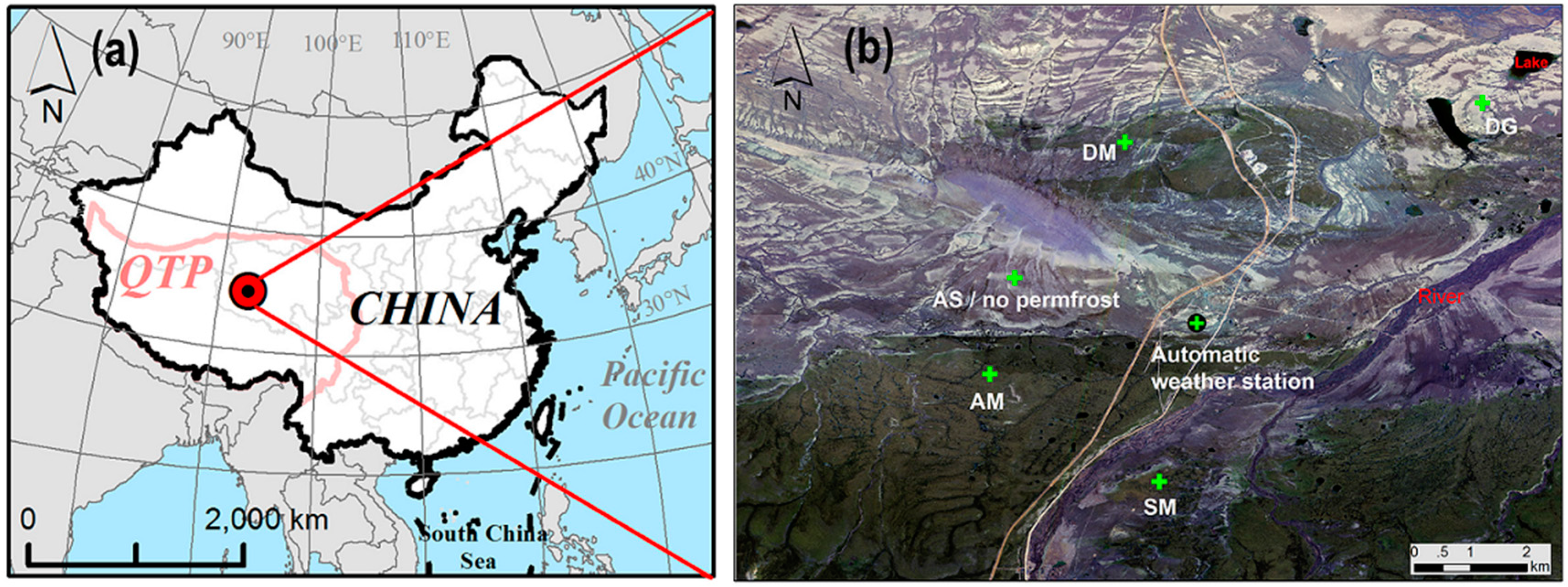
2. Study Area
3. Method
3.1. In Situ Measurements
3.2. MODIS Clear-Sky LST Data
3.3. Permafrost Thermal Modeling
3.3.1. Model description
3.3.2. Model operation
3.4. Validation Datasets
4. Results
4.1. Comparison between MODIS LST and in Situ GST and Ta
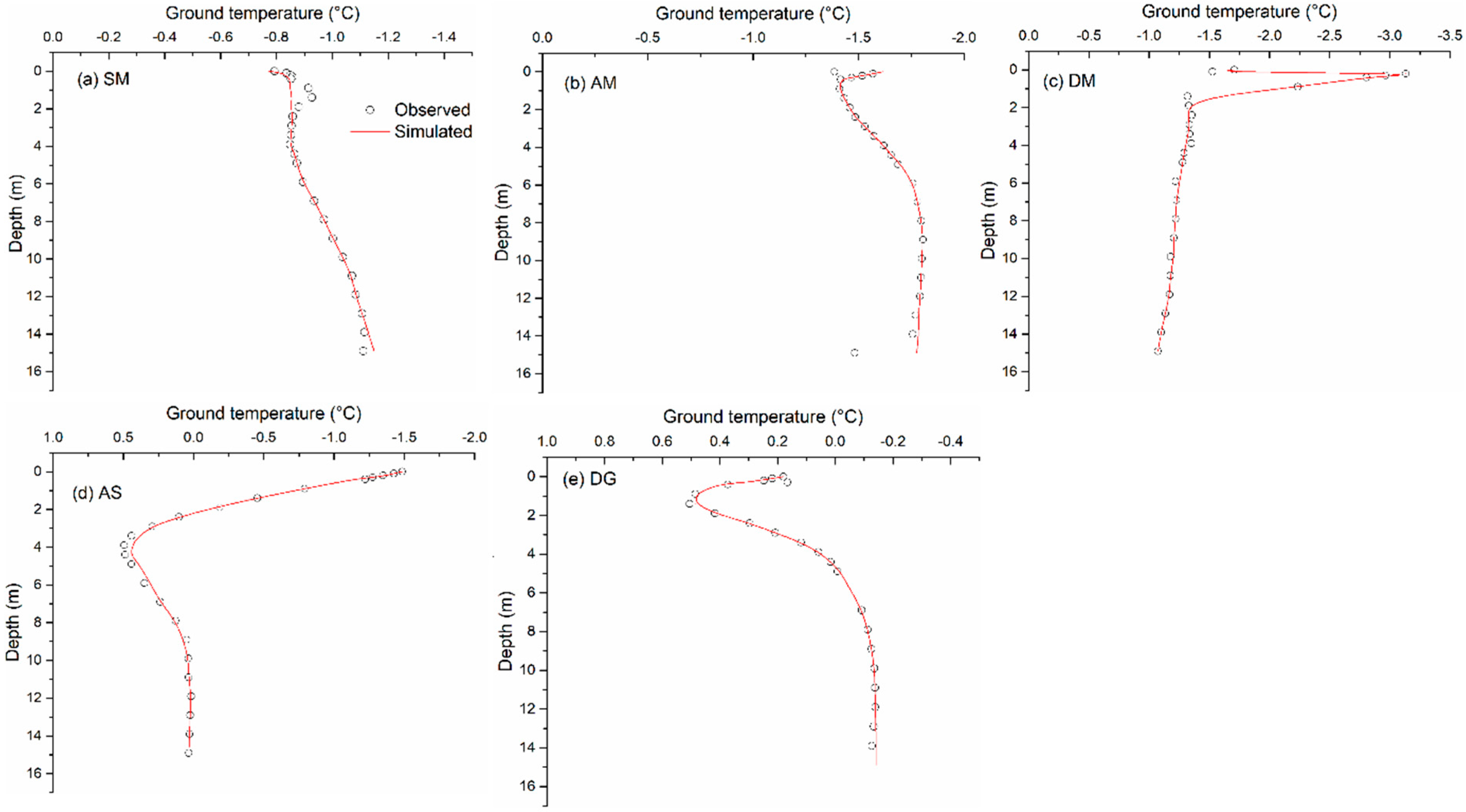
4.2. MODIS-LST-Based Modeling of Permafrost Temperature
5. Discussion
6. Conclusions
Author Contributions
Acknowledgments
Conflicts of Interest
References
- Kooi, H. Groundwater flow as a cooling agent of the continental lithosphere. Nat. Geosci. 2016, 9, 227–230. [Google Scholar] [CrossRef]
- Kurylyk, B.L.; MacQuarrie, K.T.; McKenzie, J.M. Climate change impacts on groundwater and soil temperatures in cold and temperate regions: Implications, mathematical theory, and emerging simulation tools. Earth-Sci. Rev. 2014, 138, 313–334. [Google Scholar] [CrossRef]
- Walvoord, M.A.; Kurylyk, B.L. Hydrologic Impacts of Thawing Permafrost—A Review. Vadose Zone J. 2016, 15. [Google Scholar] [CrossRef]
- Biskaborn, B.K.; Smith, S.L.; Noetzli, J.; Matthes, H.; Vieira, G.; Streletskiy, D.A.; Schoeneich, P.; Romanovsky, V.E.; Lewkowicz, A.G.; Abramov, A.Y. Permafrost is warming at a global scale. Nat. Commun. 2019, 10, 264. [Google Scholar] [CrossRef] [PubMed]
- Aalto, J.; Karjalainen, O.; Hjort, J.; Luoto, M. Statistical Forecasting of Current and Future Circum-Arctic Ground Temperatures and Active Layer Thickness. Geophys. Res. Lett. 2018, 45, 4889–4898. [Google Scholar] [CrossRef] [Green Version]
- Guo, D.; Wang, H. CMIP5 permafrost degradation projection: A comparison among different regions. J. Geophys. Res. Atmos. 2016, 121, 4499–4517. [Google Scholar] [CrossRef]
- Qiu, J. China: The third pole. Nature 2008, 454, 393–396. [Google Scholar] [CrossRef] [PubMed] [Green Version]
- Duguay, C.R.; Zhang, T.; Leverington, D.W.; Romanovsky, V.E. Satellite remote sensing of permafrost and seasonally frozen ground. Remote Sens. North. Hydrol. Meas. Environ. Chang. 2005, 163, 91–118. [Google Scholar]
- Westermann, S.; Østby, T.; Gisnås, K.; Schuler, T.; Etzelmüller, B. A ground temperature map of the North Atlantic permafrost region based on remote sensing and reanalysis data. Cryosphere 2015, 9, 1303–1319. [Google Scholar] [CrossRef] [Green Version]
- Westermann, S.; Peter, M.; Langer, M.; Schwamborn, G.; Schirrmeister, L.; Etzelmuller, B.; Boike, J. Transient modeling of the ground thermal conditions using satellite data in the Lena River delta, Siberia. Cryosphere 2016, 11, 1441–1463. [Google Scholar] [CrossRef]
- Comiso, J.C. Warming Trends in the Arctic from Clear Sky Satellite Observations. J. Clim. 2003, 16, 3498–3510. [Google Scholar] [CrossRef] [Green Version]
- Comiso, J.C. Arctic warming signals from satellite observations. Weather 2006, 61, 70–76. [Google Scholar] [CrossRef] [Green Version]
- Mialon, A.; Royer, A.; Fily, M.; Picard, G. Daily Microwave-Derived Surface Temperature over Canada/Alaska. J. Appl. Meteorol. Climatol. 2007, 46, 591–604. [Google Scholar] [CrossRef]
- Overland, J.E.; Wang, M.; Salo, S. The recent Arctic warm period. Tellus A Dyn. Meteorol. Oceanogr. 2008, 60, 589–597. [Google Scholar] [CrossRef]
- Zhang, T.; Barry, R.G.; Armstrong, R.L. Application of satellite remote sensing techniques to frozen ground studies. Polar Geogr. 2004, 28, 163–196. [Google Scholar] [CrossRef]
- Zou, D.; Zhao, L.; Yu, S.; Chen, J.; Hu, G.; Wu, T.; Wu, J.; Xie, C.; Wu, X.; Pang, Q. A new map of permafrost distribution on the Tibetan Plateau. Cryosphere 2017, 11, 2527–2542. [Google Scholar] [CrossRef] [Green Version]
- Obu, J.; Westermann, S.; Bartsch, A.; Berdnikov, N.; Christiansen, H.H.; Dashtseren, A.; Delaloye, R.; Elberling, B.; Etzelmüller, B.; Kholodov, A.; et al. Northern Hemisphere permafrost map based on TTOP modelling for 2000–2016 at 1 km2 scale. Earth-Sci. Rev. 2019, 193, 299–316. [Google Scholar] [CrossRef]
- Marchenko, S.; Hachem, S.; Romanovsky, V.; Duguay, C. Permafrost and Active Layer Modeling in the Northern Eurasia using MODIS Land Surface Temperature as an input data. In EGU General Assembly Conference Abstracts; publisher: Vienna, Austria, 2009; Volume 11, p. 11077. [Google Scholar]
- Langer, M.; Westermann, S.; Heikenfeld, M.; Dorn, W.; Boike, J. Satellite-based modeling of permafrost temperatures in a tundra lowland landscape. Remote Sens. Environ. 2013, 135, 12–24. [Google Scholar] [CrossRef] [Green Version]
- Ran, Y.; Li, X.; Jin, R.; Guo, J. Remote sensing of the mean annual surface temperature and surface frost number for mapping permafrost in China. Arct. Antarct. Alp. Res. 2015, 47, 255–265. [Google Scholar] [CrossRef]
- Yin, G.; Niu, F.; Lin, Z.; Luo, J.; Liu, M. Effects of local factors and climate on permafrost conditions and distribution in Beiluhe basin, Qinghai-Tibet Plateau, China. Sci. Total Environ. 2017, 581, 472–485. [Google Scholar] [CrossRef]
- Lin, Z.; Gao, Z.; Niu, F.; Luo, J.; Yin, G.; Liu, M.; Fan, X. High spatial density ground thermal measurements in a warming permafrost region, Beiluhe Basin, Qinghai-Tibet Plateau. Geomorphology 2019, 340, 1–14. [Google Scholar] [CrossRef]
- Wan, Z.; Dozier, J. A generalized split-window algorithm for retrieving land-surface temperature from space. IEEE Trans. Geosci. Remote Sens. 1996, 34, 892–905. [Google Scholar] [Green Version]
- Wan, Z. MODIS Land Surface Temperature Products. Available online: https://modis.gsfc.nasa.gov/ (accessed on 26 September 2019).
- Jafarov, E.E.; Marchenko, S.S.; Romanovsky, V.E. Numerical modeling of permafrost dynamics in Alaska using a high spatial resolution dataset. Cryosphere 2012, 6, 613–624. [Google Scholar] [CrossRef] [Green Version]
- Wu, Q.; Zhang, T.; Liu, Y. Permafrost temperatures and thickness on the Qinghai-Tibet Plateau. Glob. Planet. Chang. 2010, 72, 32–38. [Google Scholar] [CrossRef]
- Adolph, A.C.; Albert, M.R.; Hall, D.K. Near-surface temperature inversion during summer at Summit, Greenland, and its relation to MODIS-derived surface temperatures. Cryosphere 2018, 12, 907–920. [Google Scholar] [CrossRef] [Green Version]
- Liu, Y.; Ackerman, S.A.; Maddux, B.; Key, J.R.; Frey, R.A. Errors in Cloud Detection over the Arctic Using a Satellite Imager and Implications for Observing Feedback Mechanisms. J. Clim. 2010, 23, 1894–1907. [Google Scholar] [CrossRef] [Green Version]
- Westermann, S.; Langer, M.; Boike, J. Spatial and temporal variations of summer surface temperatures of high-arctic tundra on Svalbard—Implications for MODIS LST based permafrost monitoring. Remote Sens. Environ. 2011, 115, 908–922. [Google Scholar] [CrossRef]
- Hachem, S.; Allard, M.; Duguay, C. Using the MODIS land surface temperature product for mapping permafrost: An application to northern Québec and Labrador, Canada. Permafr. Periglac. Process. 2009, 20, 407–416. [Google Scholar] [CrossRef]
- Hall, D.K.; Box, J.E.; Casey, K.A.; Hook, S.J.; Shuman, C.A.; Steffen, K. Comparison of satellite-derived and in-situ observations of ice and snow surface temperatures over Greenland. Remote Sens. Environ. 2008, 112, 3739–3749. [Google Scholar] [CrossRef] [Green Version]
- Lin, Z.; Burn, C.R.; Niu, F.; Luo, J.; Liu, M.; Yin, G. The thermal regime, including a reversed thermal offset, of arid permafrost sites with variations in vegetation cover density, Wudaoliang Basin, Qinghai-Tibet plateau. Permafr. Periglac. Process. 2015, 26, 142–159. [Google Scholar] [CrossRef]
- Zhang, Y.; Wang, X.; Fraser, R.; Olthof, I.; Chen, W.; Mclennan, D.; Ponomarenko, S.; Wu, W. Modelling and mapping climate change impacts on permafrost at high spatial resolution for an Arctic region with complex terrain. Cryosphere 2013, 7, 1121–1137. [Google Scholar] [CrossRef] [Green Version]
- Nicolsky, D.J.; Romanovsky, V.; Panda, S.; Marchenko, S.; Muskett, R. Applicability of the ecosystem type approach to model permafrost dynamics across the Alaska North Slope. J. Geophys. Res. Earth Surf. 2017, 122, 50–75. [Google Scholar] [CrossRef]
- Luo, J.; Yin, G.; Niu, F.; Lin, Z.; Liu, M. High Spatial Resolution Modeling of Climate Change Impacts on Permafrost Thermal Conditions for the Beiluhe Basin, Qinghai-Tibet Plateau. Remote Sens. 2019, 11, 1294. [Google Scholar] [CrossRef]


| Soil Layer | VWC | UWC | C (106 Jm−3K−1) | K (Wm−1K−1) | Depth (m) | |||
|---|---|---|---|---|---|---|---|---|
| a | b | Ct | Cf | kt | kf | |||
| SM | ||||||||
| Sand | 0.20 | 0.07 | −0.17 | 3.1 | 1.5 | 1.5 | 0.9 | 0–1 |
| Clay | 0.18 | 0.12 | −0.15 | 2.5 | 1.9 | 1.7 | 2.2 | 1–10 |
| Rock | 0.04 | 0.01 | −0.1 | 3.25 | 2.48 | 2.7 | 3.1 | >10 |
| AM | ||||||||
| Sand | 0.18 | 0.07 | −0.17 | 3.1 | 1.5 | 1.6 | 2.4 | 0–2 |
| Clay | 0.17 | 0.12 | −0.15 | 2.5 | 1.9 | 0.7 | 1.4 | 2–10 |
| Bedrock | 0.04 | 0.01 | −0.1 | 3.25 | 2.48 | 2.7 | 3.1 | >10 |
| DM | ||||||||
| Sand | 0.06 | 0.037 | −0.14 | 2.8 | 2.2 | 1.3 | 1.6 | 0–2 |
| Clay | 0.12 | 0.12 | −0.15 | 2.5 | 1.9 | 1.3 | 1.6 | 2–10 |
| Rock | 0.04 | 0.01 | −0.1 | 3.25 | 2.48 | 2.7 | 3.1 | >10 |
| AS | ||||||||
| Sand with gravel | 0.12 | 0.037 | −0.14 | 2.8 | 2.2 | 1.3 | 1.6 | 0–3 |
| Clay | 0.12 | 0.12 | −0.15 | 2.5 | 1.9 | 0.6 | 1.0 | 3–10 |
| Rock | 0.04 | 0.01 | −0.1 | 3.25 | 2.48 | 2.7 | 3.1 | >10 |
| DG | ||||||||
| Sand | 0.1 | 0.05 | −0.17 | 3.1 | 1.5 | 1.3 | 1.6 | 0–5 |
| Clay | 0.12 | 0.12 | −0.15 | 2.5 | 1.9 | 0.6 | 1.0 | 5–10 |
| Rock | 0.04 | 0.01 | −0.1 | 3.25 | 2.48 | 2.7 | 3.1 | >10 |
| Site | R2 | MD (°C) | SD (°C) | |
|---|---|---|---|---|
| Ta/GST | Ta/GST | Ta/GST | ||
| SM | MOD | 0.87/0.81 | −4.57/−0.98 | 3.61/5.65 |
| MYD | 0.88/0.82 | −4.38/−0.98 | 3.45/5.64 | |
| MOD/MYD | 0.94/0.87 | −4.65/−0.81 | 2.61/5.39 | |
| AM | MOD | 0.85/0.86 | −4.43/−2.58 | 3.66/3.73 |
| MYD | 0.87/0.86 | −3.99/−2.32 | 3.46/3.71 | |
| MOD/MYD | 0.92/0.91 | −4.43/−2.66 | 2.76/3.11 | |
| DM | MOD | 0.85/0.83 | −4.14/−2.21 | 3.80/4.46 |
| MYD | 0.86/0.84 | −4.48/−2.62 | 3.51/4.22 | |
| MOD/MYD | 0.91/0.89 | −4.46/−2.53 | 2.89/3.95 | |
| AS | MOD | 0.85/0.83 | −4.58/−0.91 | 4.03/3.98 |
| MYD | 0.85/0.85 | −3.93/−0.12 | 3.88/3.75 | |
| MOD/MYD | 0.92/0.91 | −4.67/−0.67 | 3.02/2.98 | |
| DG | MOD | 0.86/0.88 | −4.76/−1.22 | 3.99/3.65 |
| MYD | 0.85/0.86 | −4.47/−0.62 | 4.03/3.84 | |
| MOD/MYD | 0.92/0.93 | −4.73/−1.05 | 3.12/2.88 |
| Site | Depth | R2 | ME | RMSE |
|---|---|---|---|---|
| SM | 3 | 0.90 | 0.12 | 0.35 |
| 10 | 0.93 | 0.11 | 0.25 | |
| AM | 3 | 0.96 | 0.11 | 0.32 |
| 10 | 0.92 | 0.10 | 0.26 | |
| DM | 3 | 0.94 | 0.10 | 0.21 |
| 10 | 0.75 | 0.05 | 0.02 | |
| AS | 3 | 0.91 | 0.82 | 0.53 |
| 10 | 0.89 | 0.08 | 0.22 | |
| DG | 3 | 0.83 | 0.06 | 0.1 |
| 10 | 0.90 | 0.02 | 0.1 |
| Site | Simulated ALT (m) | Measured ALT (m) | Difference (m) |
|---|---|---|---|
| SM | 1.75 | 1.40 | 0.35 |
| AM | 1.90 | 1.80 | 0.10 |
| DM | 1.60 | 1.80 | 0.20 |
| AS | No permafrost | No permafrost | / |
| DG | 3.20 | 3.40 | 0.20 |
© 2019 by the authors. Licensee MDPI, Basel, Switzerland. This article is an open access article distributed under the terms and conditions of the Creative Commons Attribution (CC BY) license (http://creativecommons.org/licenses/by/4.0/).
Share and Cite
Li, A.; Xia, C.; Bao, C.; Yin, G. Using MODIS Land Surface Temperatures for Permafrost Thermal Modeling in Beiluhe Basin on the Qinghai-Tibet Plateau. Sensors 2019, 19, 4200. https://doi.org/10.3390/s19194200
Li A, Xia C, Bao C, Yin G. Using MODIS Land Surface Temperatures for Permafrost Thermal Modeling in Beiluhe Basin on the Qinghai-Tibet Plateau. Sensors. 2019; 19(19):4200. https://doi.org/10.3390/s19194200
Chicago/Turabian StyleLi, Anyuan, Caichu Xia, Chunyan Bao, and Guoan Yin. 2019. "Using MODIS Land Surface Temperatures for Permafrost Thermal Modeling in Beiluhe Basin on the Qinghai-Tibet Plateau" Sensors 19, no. 19: 4200. https://doi.org/10.3390/s19194200
APA StyleLi, A., Xia, C., Bao, C., & Yin, G. (2019). Using MODIS Land Surface Temperatures for Permafrost Thermal Modeling in Beiluhe Basin on the Qinghai-Tibet Plateau. Sensors, 19(19), 4200. https://doi.org/10.3390/s19194200