Reducing the Effect of Positioning Errors on Kinematic Raw Doppler (RD) Velocity Estimation Using BDS-2 Precise Point Positioning

Abstract
1. Introduction
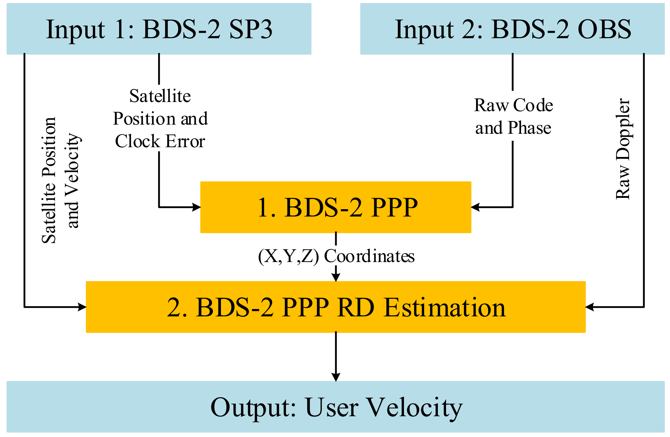
2. Methodology of the Proposed BDS-2 PPP-Based RD Velocity Estimation
3. Experiments and Analysis
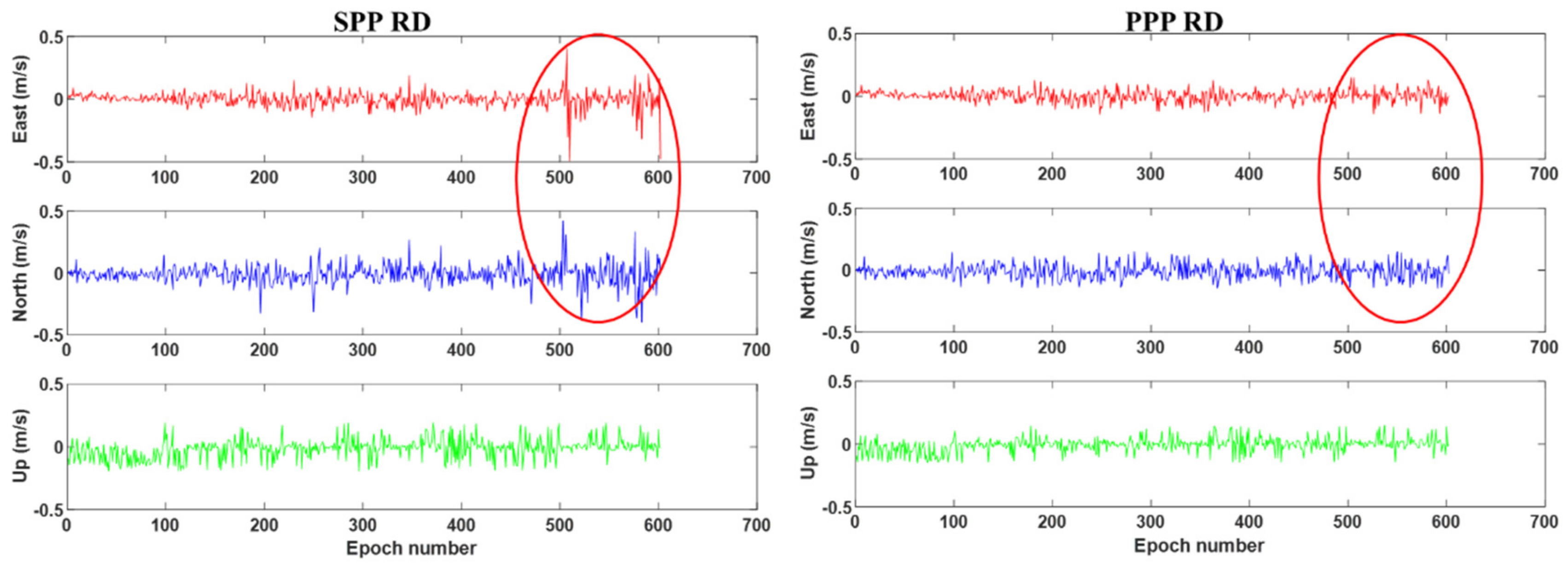
3.1. Vehicle-Borne Experiment
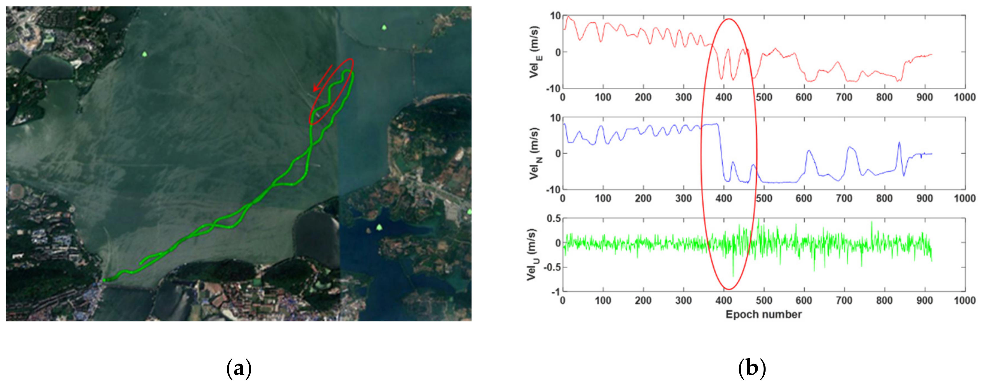
3.2. Ship-Borne Experiment
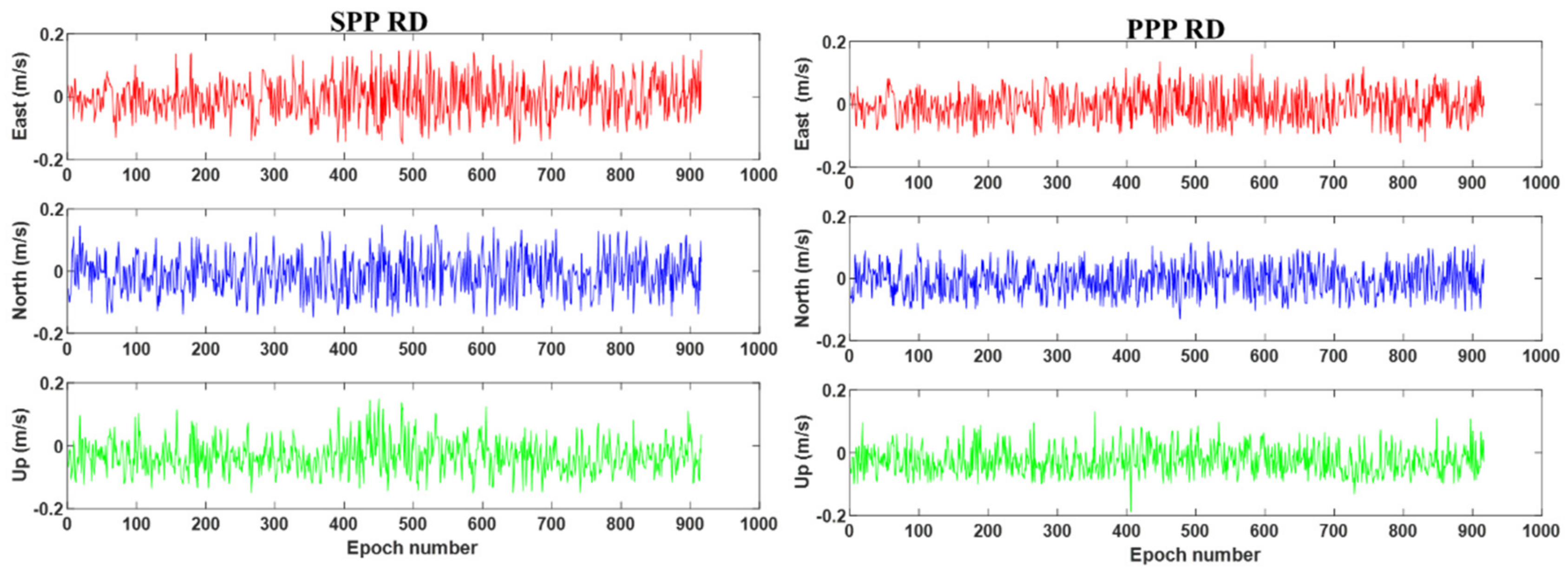
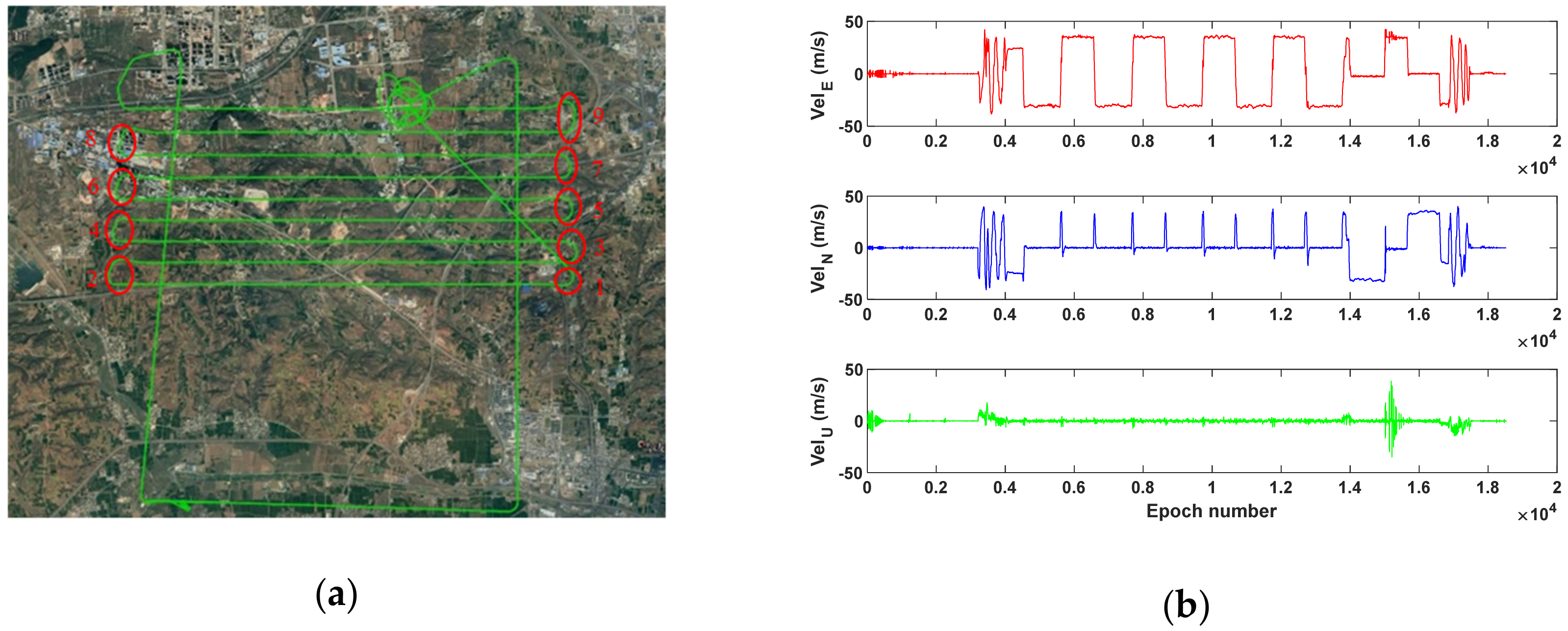
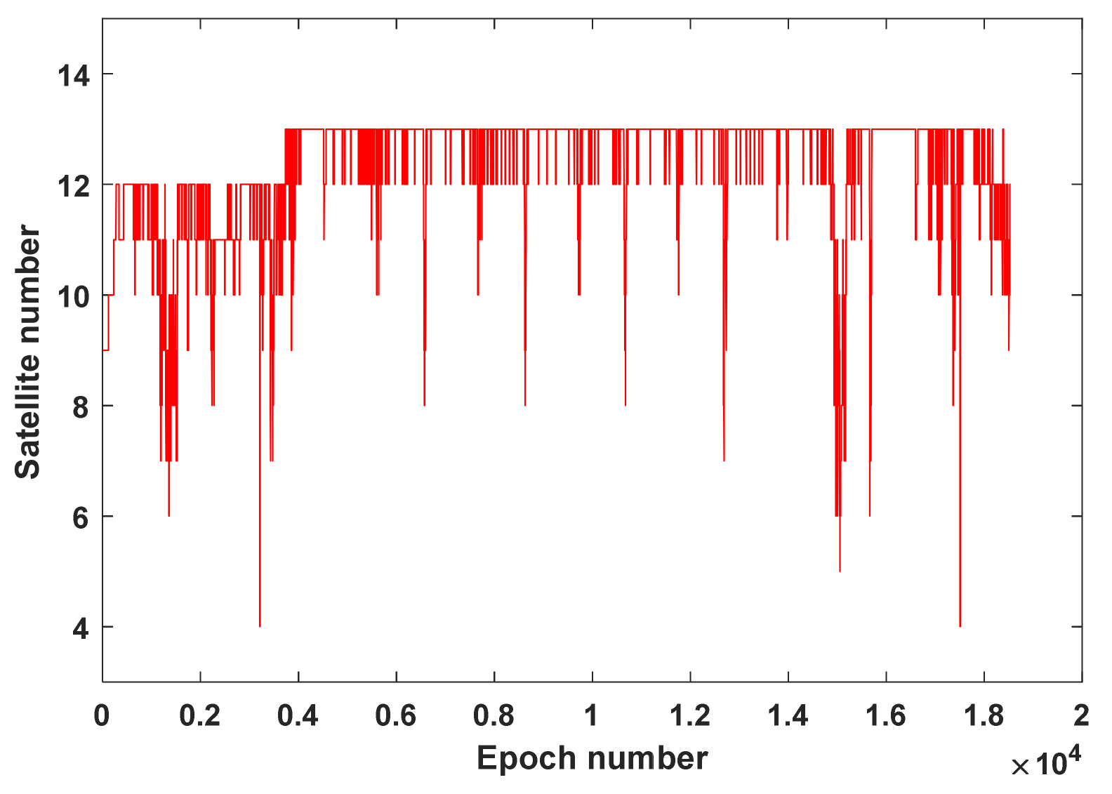
3.3. Air-Borne Experiment
4. Conclusions
Author Contributions
Funding
Acknowledgments
Conflicts of Interest
References
- He, H.; Yang, Y.; Sun, Z. A comparison of several approaches for velocity determination with GPS. Acta Cartogr. Sin. 2002, 31, 217–221. [Google Scholar]
- Li, M.; Neumayer, K.H.; Flechtner, F.; Lu, B. Performance Assessment of Multi-GNSS Precise Velocity and Acceleration Determination over Antarctica. J. Navig. 2019, 7, 1–18. [Google Scholar] [CrossRef]
- Szarmes, M.; Ryan, S.; Lachapelle, G. DGPS high accuracy aircraft velocity determination using Doppler measurements. In Proceedings of the International Symposium on Kinematic Systems (KIS), Bannf, AB, Canada, 4–6 June 1997. [Google Scholar]
- Wang, F.; Zhang, X.; Huang, J. Error analysis and accuracy assessment of GPS absolute velocity determination with SA off. Geomat. Inform. Sci. Wuhan Univ. 2007, 32, 515–519. [Google Scholar]
- Liu, Z.; Chen, G.; Zhao, Q. Principle and precision analysis of BDS absolute velocity determination. J. Geod. Geom. 2014, 34, 114–118. [Google Scholar]
- Zheng, K.; Tang, L. Performance Assessment of BDS and GPS/BDS Velocity Estimation with Stand-alone Receiver. J. Navig. 2016, 69, 869–882. [Google Scholar] [CrossRef]
- Li, X.; Guo, J.; Zhang, D. An Algorithm of GPS Single-Epoch Kinematic Positioning Based on Doppler Velocimetry. Geomat. Inform. Sci. Wuhan Univ. 2018, 43, 1036–1041. [Google Scholar]
- Zhang, X.; Guo, B. Real-time tracking the instantaneous movement of crust during earthquake with a stand-alone GPS receiver. Chin. J. Geop. 2013, 56, 1928–1936. [Google Scholar]
- Li, M.; Li, W.; Fang, R.; Shi, C. Real-time high-precision earthquake monitoring using single-frequency GPS receivers. GPS Solut. 2015, 19, 27–35. [Google Scholar] [CrossRef]
- Zhang, X.; Guo, B.; Guo, F.; Du, C. Influence of clock jump on the velocity and acceleration estimation with a single GPS receiver based on carrier-phase-derived Doppler. GPS Solut. 2013, 17, 549–559. [Google Scholar] [CrossRef]
- Ye, S.; Yan, Y.; Chen, D. Performance analysis of velocity estimation with BDS. J. Navig. 2017, 70, 580–594. [Google Scholar] [CrossRef]
- Graas Van, F.; Soloviev, A. Precise velocity estimation using a stand-alone GPS receiver. J. Navig. 2004, 51, 283–292. [Google Scholar] [CrossRef]
- Wendel, J.; Meister, O.; Moenikes, R.; Trommer, G.F. Time differenced carrier phase measurements for tightly coupled GPS/INS integration. In Proceedings of the IEEE/ION PLANS, San Diego, CA, USA, 25–27 April 2006; pp. 54–60. [Google Scholar]
- Soon, B.K.H.; Scheding, S.; Lee, H.K.; Lee, H.K.; Durrant-Whyte, H. An approach to aid INS using time-differenced GPS carrier phase (TDCP) measurements. GPS Solut. 2008, 12, 261–271. [Google Scholar] [CrossRef]
- Freda, P.; Angrisano, A.; Gaglione, S.; Troisi, S. Time-differenced carrier phases technique for precise GNSS velocity estimation. GPS Solut. 2015, 19, 335–341. [Google Scholar] [CrossRef]
- Odolinski, R.; Teunissen, P.J.G.; Odijk, D. Combined GPS + BDS for short to long baseline RTK positioning. Meas. Sci. Technol. 2015, 26, 045801. [Google Scholar] [CrossRef]
- Wang, K.; Chen, P.; Teunissen, P.J.G. Single-Epoch, Single-Frequency Multi-GNSS L5 RTK under High-Elevation Masking. Sensors 2019, 19, 1066. [Google Scholar] [CrossRef] [PubMed]
- Ge, Y.; Dai, P.; Qin, W.; Yang, X.; Zhou, F.; Wang, S.; Zhao, X. Performance of Multi-GNSS Precise Point Positioning Time and Frequency Transfer with Clock Modeling. Remote Sens. 2019, 11, 347. [Google Scholar] [CrossRef]
- Shi, J.; Wang, G.; Han, X.; Guo, J. Impacts of Satellite Orbit and Clock on Real-Time GPS Point and Relative Positioning. Sensors 2017, 17, 1363. [Google Scholar] [CrossRef]
- Yu, X.; Gao, J. Kinematic Precise Point Positioning Using Multi-Constellation Global Navigation Satellite System (GNSS) Observations. ISPRS Int. J. Geo-Inf. 2017, 6, 6. [Google Scholar] [CrossRef]
- Wang, Z.; Li, Z.; Wang, L.; Wang, X.; Yuan, H. Assessment of Multiple GNSS Real-Time SSR Products from Different Analysis Centers. ISPRS Int. J. Geo-Inf. 2018, 7, 85. [Google Scholar] [CrossRef]
- Aggrey, J.; Bisnath, S. Improving GNSS PPP Convergence: The Case of Atmospheric-Constrained, Multi-GNSS PPP-AR. Sensors 2019, 19, 587. [Google Scholar] [CrossRef]
- Shi, J.; Gao, Y. A comparison of three PPP integer ambiguity resolution methods. GPS Solut. 2014, 18, 519–528. [Google Scholar] [CrossRef]
- Du, S.; Gao, Y. Inertial Aided Cycle Slip Detection and Identification for Integrated PPP GPS and INS. Sensors 2012, 12, 14344–14362. [Google Scholar] [CrossRef] [PubMed]
- Ouyang, C.; Shi, J.; Shen, Y.; Li, L. Six-Year BDS-2 Broadcast Navigation Message Analysis from 2013 to 2018: Availability, Anomaly, and SIS UREs Assessment. Sensors 2019, 19, 2767. [Google Scholar] [CrossRef] [PubMed]


| Method | Static (RMS) | Kinematic (RMS) | Estimated Velocity |
|---|---|---|---|
| PD | mm/s–cm/s | cm/s–m/s | Average between two epochs |
| RD | mm/s–cm/s | mm/s–cm/s | Instantaneous at current epoch |
| DD | mm/s | cm/s–dm/s | Average between two epochs |
| TDCP | mm/s | cm/s–dm/s | Average between two epochs |
| Vehicle-Borne | Ship-Borne | Air-Borne | |
|---|---|---|---|
| UTC | 2018/11/6/ 7:04–7:14 | 2016/6/14/ 8:16–8:32 | 2016/6/15/ 8:00–9:02 |
| Location | 42°02′ N 121°39′E | 30°32′N 114°23′E | 34°25′N 113°05′E |
| Sampling | 1 Hz | 1 Hz | 5 Hz |
| Receiver | NovAtel OEM4 | ComNav K505 | NovAtel OEM4 |
| Velocity | ~20 m/s | ~15 m/s | ~40 m/s |
| Reference | BDS/GPS RTK + INS | BDS/GPS RTK PD | BDS/GPS RTK PD |
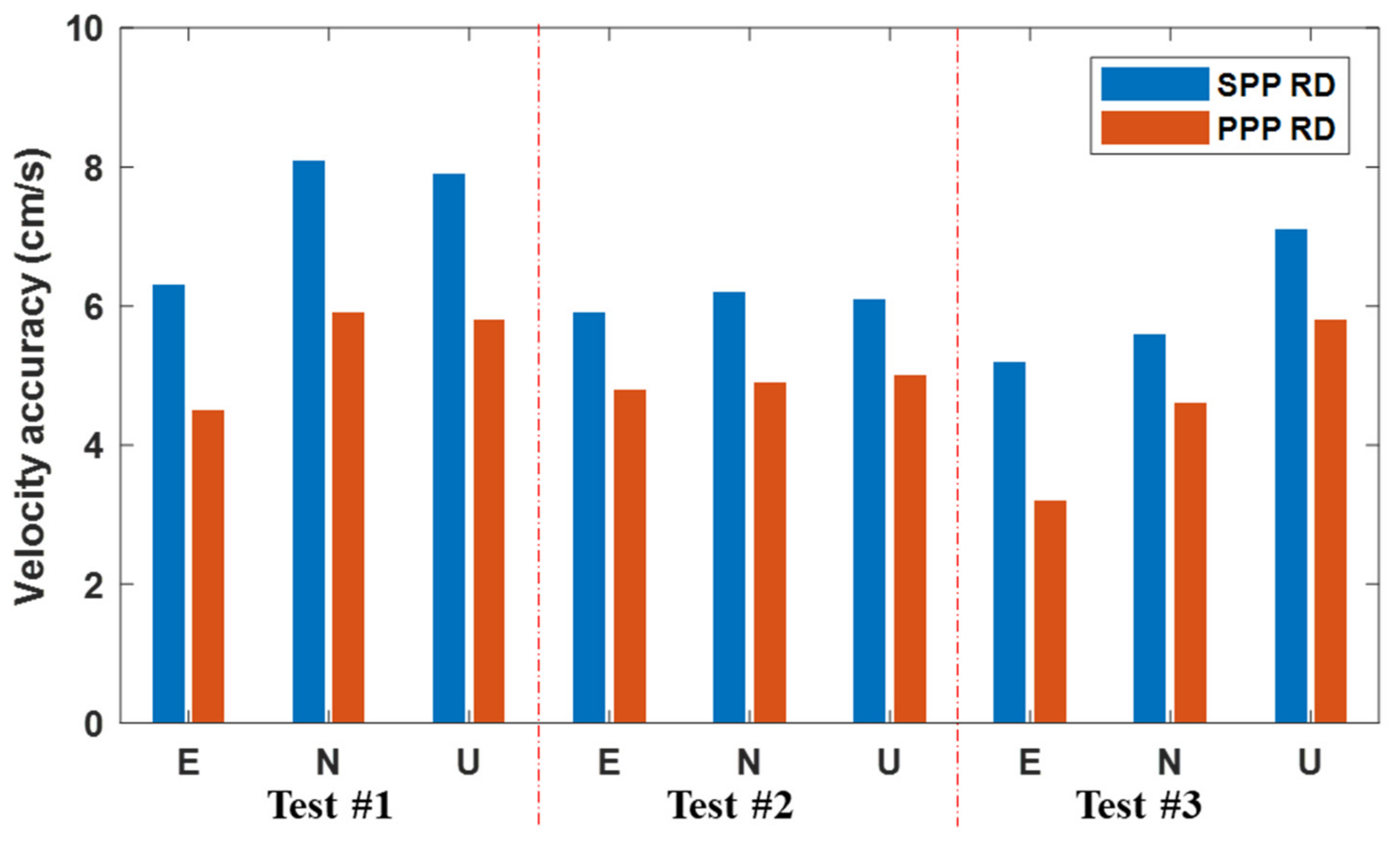
| SPP RD (cm/s) | PPP RD (cm/s) | Improvement (%) | |
|---|---|---|---|
| East | 6.3 | 4.5 | 28.4 |
| North | 8.1 | 5.9 | 27.1 |
| Up | 7.9 | 5.8 | 26.1 |
| SPP RD (cm/s) | PPP RD (cm/s) | Improvement (%) | |
|---|---|---|---|
| East | 5.9 | 4.8 | 17.4 |
| North | 6.2 | 4.9 | 21.4 |
| Up | 6.1 | 5 | 17.8 |
| SPP RD (cm/s) | PPP RD (cm/s) | Improvement (%) | |
|---|---|---|---|
| East | 5.2 | 3.2 | 38.1 |
| North | 5.6 | 4.6 | 17.6 |
| Up | 7.1 | 5.8 | 17.5 |
© 2019 by the authors. Licensee MDPI, Basel, Switzerland. This article is an open access article distributed under the terms and conditions of the Creative Commons Attribution (CC BY) license (http://creativecommons.org/licenses/by/4.0/).
Share and Cite
Duan, S.; Sun, W.; Ouyang, C.; Chen, X.; Shi, J. Reducing the Effect of Positioning Errors on Kinematic Raw Doppler (RD) Velocity Estimation Using BDS-2 Precise Point Positioning. Sensors 2019, 19, 3029. https://doi.org/10.3390/s19133029
Duan S, Sun W, Ouyang C, Chen X, Shi J. Reducing the Effect of Positioning Errors on Kinematic Raw Doppler (RD) Velocity Estimation Using BDS-2 Precise Point Positioning. Sensors. 2019; 19(13):3029. https://doi.org/10.3390/s19133029
Chicago/Turabian StyleDuan, Shunli, Wei Sun, Chenhao Ouyang, Xinyu Chen, and Junbo Shi. 2019. "Reducing the Effect of Positioning Errors on Kinematic Raw Doppler (RD) Velocity Estimation Using BDS-2 Precise Point Positioning" Sensors 19, no. 13: 3029. https://doi.org/10.3390/s19133029
APA StyleDuan, S., Sun, W., Ouyang, C., Chen, X., & Shi, J. (2019). Reducing the Effect of Positioning Errors on Kinematic Raw Doppler (RD) Velocity Estimation Using BDS-2 Precise Point Positioning. Sensors, 19(13), 3029. https://doi.org/10.3390/s19133029