Article

Computer Vision Classification of Barley Flour Based on Spatial Pyramid Partition Ensemble

by
Jessica Fernandes Lopes
1,
Leniza Ludwig
2,
Douglas Fernandes Barbin
3,
Maria Victória Eiras Grossmann
2 and
Sylvio Barbon, Jr.
1,*
1
Department of Computer Science, Londrina State University (UEL), Londrina 86057-970, Brazil
2
Department of Food Sciences, Londrina State University (UEL), Londrina 86057-970, Brazil
3
Department of Food Engineering, University of Campinas, Campinas 13083-970, Brazil
*
Author to whom correspondence should be addressed.
Sensors 2019, 19(13), 2953; https://doi.org/10.3390/s19132953
Submission received: 12 March 2019 / Revised: 24 April 2019 / Accepted: 13 May 2019 / Published: 4 July 2019
(This article belongs to the Section Remote Sensors)

Abstract

:
Imaging sensors are largely employed in the food processing industry for quality control. Flour from malting barley varieties is a valuable ingredient in the food industry, but its use is restricted due to quality aspects such as color variations and the presence of husk fragments. On the other hand, naked varieties present superior quality with better visual appearance and nutritional composition for human consumption. Computer Vision Systems (CVS) can provide an automatic and precise classification of samples, but identification of grain and flour characteristics require more specialized methods. In this paper, we propose CVS combined with the Spatial Pyramid Partition ensemble (SPPe) technique to distinguish between naked and malting types of twenty-two flour varieties using image features and machine learning. SPPe leverages the analysis of patterns from different spatial regions, providing more reliable classification. Support Vector Machine (SVM), k-Nearest Neighbors (k-NN), J48 decision tree, and Random Forest (RF) were compared for samples’ classification. Machine learning algorithms embedded in the CVS were induced based on 55 image features. The results ranged from 75.00% (k-NN) to 100.00% (J48) accuracy, showing that sample assessment by CVS with SPPe was highly accurate, representing a potential technique for automatic barley flour classification.

1. Introduction

Barley is one of the most ancient cereal crops grown by humanity [1]. Over the years, some barley cultivars (e.g. malting or hulled barley) were selected for the malt and brewery industry, while other cultivars were selected to be used as food ingredients. These last cultivars are known as naked, or even hull-less or uncovered barley, generally containing higher amounts of soluble fiber [2,3]. Requirements concerning barley characteristics are quite different for malting and food industries. For brewery, grains with a low β -glucan concentration and barley kernels with a tough inedible outer hull still attached are required. High β -glucan levels interfere negatively in the malting filtration process. Furthermore, the loss of husks during malting processes leads to a reduction in malt quality. Such characteristics are inherent in hulled varieties [4]. On the other hand, barley cultivars with high levels of proteins and β -glucan (a functional ingredient) are preferred in the food industry, and some further specifications may vary depending on the requirements of each product. As an example, flours from naked types are preferably used for infant foods because they generally have fewer husk fragments [5].
Due to vast applicability, barley is one of the four significant grains, being used for various organic food materials [6,7]. Despite the genetic resource of a variety being the significant factor in determining its technological characteristics, it is well established that environmental conditions and interactions between environment and genotype can modify the expression of such characteristics [8]. Consequently, it is difficult to predict the best industrial destination for barley, or other cereal grains, without performing some physical and chemical analysis, which are generally expensive, time-consuming, and/or require specialized analysts and equipment [9]. The agricultural and food industries are often searching for fast and accurate technologies to increase processing performance, improving product quality. Imaging sensors and computer vision systems have been developed for grading product quality, discriminating among varieties, and detecting contaminants or added substances [10,11,12].
Quality evaluation can be performed by a Computer Vision System (CVS) based on an acquisition device (digital camera, inexpensive and broadly available) and prediction models using machine learning algorithms. This type of approach presents several advantages, including rapidity, low cost, and accuracy and can be applied to grains/seeds [13,14], flours [11], or other agricultural by-products. Being non-invasive methods and not employing chemical reagents, they can be considered as eco-friendly technologies. Product inspection is in high demand in the food industry, including quality inspection, process control, classification, and grading. Manual inspection by visual examination demands a long time and is tedious and inefficient. Machine vision is suitable for this task, as computer vision provides an economical and fast alternative for food processing inspection [15].
The visual aspect is one of the most important parameters for the assessment of food quality. The general utilization of processing equipment in the industry has increased the risk of foreign material contamination [16]. Adulteration, contamination, or simply grading of products according to their visual characteristics are a common need in food processing. For instance, due to the resulting potential health threat to consumers, the development of a fast, label-free, and non-invasive technique for the detection of adulteration over a wide range of food products is necessary [17]. Hence, the food industry is interested in optimizing not only the nutritional characteristics of food products, but also their appearance, including color, texture, etc. It is essential to investigate objective methods that can quantify the visual aspects of food products [18].
To meet the demand for high-quality produce, grains are classified according to their characteristics, before being sent for processing. Manual inspection of in-process products is difficult considering the sampling from processing lines [15]. Considering that barley grains are inhomogeneous, imaging techniques will have extensive practical applicability as analytical tools during industrial processing. Regarding all the chemical-free techniques available, there are still some common challenges before transferring recent research achievements obtained from a laboratory scale to industrial applications, such as building innovative data analysis algorithms that can thoroughly filter redundant information; exploiting appropriate statistical techniques for improving the model robustness for real-time operations; and decreasing the cost of the instrument [19].
In digital image analysis, spatial pyramid methods are very popular for preserving the spatial information of local features, focusing on improving the pattern description [20]. Sharma et al. [21] proposed Spatial Pyramid Partition (SPP) and highlighted that in many visual classification tasks, the spatial distribution carries important information for a given visual classification task. However, the proposed SPP method based on bag of features leads to enlarging the feature vector when several image descriptors take place, resulting in a highly dimensional problem and demanding feature extraction or feature selection methods.
Szczypinski et al. [9] classified barley grain varieties based on image-derived shape, color, and texture attributes of individual kernels. Considering barley flour classification, spatial information is required, but the original SPP is not feasible in our problem due to the characteristics of bag of features. In other words, barley grain and flour image-based classification demand several features, while flour image analysis requires more robust pattern recognition approaches than SPP can provide. However, the increase of dimensionality arising from the application of SPP is a challenge in the machine learning scenario, and consequently for CVS applications. Therefore, we proposed the Spatial Pyramid Partition ensemble (SPPe), an ensemble technique fashioned on SPP towards supporting a suitable image pattern description in scenarios with a considerable number of features, as exposed in Figure 1.
A vast number of characteristics might rely on performance improvement of prediction tasks. The traditional feature extraction method considers the whole image at once for extracting its features, which possibly decreases important spatial information of some image descriptors from samples. As previously mentioned, the SPP was proposed to improve the problem task that requires some localized descriptors. However, it is based on a bag of features grounded on splitting images into sub-regions for supporting additional spatial information. Thus, SPP appraises a visual descriptor vector composed by the original image and its sub-regions from each sample.
The proposed SPPe was evaluated in a CVS with a set of image features based on color, intensity, and texture, in comparison to SPP [21], directly using the features extracted from the Region Of Interest (ROI), as traditional CVS [13,22,23,24]. We compared the performance of four different machine learning algorithms: Random Forest (RF), Support Vector Machine (SVM), k Nearest Neighbor (k-NN), and J48 decision tree for modeling the classifier. These algorithms were employed to distinguish between naked and malting barley flour with image features extracted from 22 varieties acquired from five samples of each variety.

2. Related Work

Several studies presented CVS with machine learning methods applied to improve the prediction of a given parameter. Some CVS require sophisticated modeling to cope with non-linearities and noisy and imbalanced datasets. The application of Machine Learning (ML) techniques for food attributes’ prediction and quality evaluation has been widely investigated [10,22,25,26,27,28,29,30]. ML can be applied to extract non-trivial relationships automatically from a training dataset, producing a generalization of knowledge for further predictions [31]. Hence, machine learning promotes high performance as an alternative for an intensive agricultural operational process of the agri-technologies domain [32].
Random Forest (RF) [33], Support Vector Machine (SVM) [34], k-Nearest Neighbors (k-NN) [35], and the J48 decision tree algorithm [36] are well-established machine learning algorithms applied in many studies related to food quality analyses. RF was compared to SVM for an automated marbling grading system of dry-cured ham [37]. The SVM algorithm showed better performance with 89 % of the samples correctly classified. Another application of SVM was described in Papadopulou et al. [27], achieving over 89 % of accuracy for classification of beef fillets according to quality grades. For analyzing image features to evaluate the impact of diets on live fish skin, Saberioon et al. [38] applied four different classification methods, and SVM provided the best classifier with 82 % of accuracy. Barbon et al. [23] proposed a CVS for meat classification based on image features, managed by an instance-based system using k-NN to classify meat according to marbling scores from image features. The authors presented an accuracy of 81 . 59 % for bovine and 76 . 14 % for swine samples, using only three samples for each marbling score by the k-NN prediction models. Granitto et al. [30] applied RF for the discrimination of six different Italian cheeses. In addition to reasonable accuracy, the RF model provided an estimation of the relative importance of each sensory attribute involved. The effectiveness of RF was also highlighted in a CVS used for predicting the ripening of papaya from digital imaging [22].
Considering barley applications, Nowakowski et al. [39] evaluated malt barley seeds using four barley varieties. The feasibility of image analysis was applied with machine learning and morphology and color features, achieving 99% accuracy. Kociolek et al. [40] classified barley grain defects using preprocessed kernel image pairs for feature extraction based on morphological operations. Pazoki et al. [41] identified cultivars using rain-fed barley seeds. The proposed method was applied with 22 features extracted from three varieties of samples, which fed a Multilayer Perceptron (MLP). The features of color, morphology, and shape were used for individual rain-fed barley seeds. Different network architectures were explored, including feature selection, resulting in 82 . 22 % accuracy. Ciesielski and Nguyen [42] proposed to distinguish three different classes of bulk malt (made by barley grains). Image texture features were extracted and classification was performed with k-nearest-neighbor (k-NN), achieving an accuracy of 77 . 00 % . According to the authors, the classification through the evaluation of individual kernels is time-consuming, and many kernels are required to obtain a significant estimation of the modification index from a whole batch. Nevertheless, separating the samples in minimal milling portions is a booster alternative, aiding the evaluation of the difference between barley types. Lim et al. [7] explored Near Infrared Spectroscopy (NIRS) and a PLS-DA discrimination model to predict hulled barley, naked barley, and wheat contaminated with Fusarium. The authors achieved high accuracy at the cost of the complexity of NIRS equipment and signal processing.
Accordingly, the above studies have performed image analysis at different stages for varieties’ identification for industrialization and improvement purposes. Integrating the industrial environment promotes a major role for developing an automated system for distinguishing agricultural raw-material products. The approach introduced in this paper is a CVS with an adaptation of the original SPP, modifying the overview perspective of sub-images that compose an original sample. The proposed approach is based on splitting each image into several sub-regions to predict a respective sample. We propose a method to improve prediction performance using CVS with machine learning, by applying the SPPe technique.

3. Materials and Methods

Twenty-two different barley varieties (cultivars) were provided by EMBRAPA Trigo (Brazilian Agricultural Research Corporation) in the city of Passo Fundo (Brazil). Barley samples were dehulled (Codema Inc. equipment, Maple Grove, MN, USA) during 75 s and milled (IKA A11 Basic Micro Miller, Osaka, Japan) for 75 s. Five different color images of flour were acquired from each of the 22 cultivars, in a total of 110 samples. Samples were collected and labeled by a specialist according to the source types of barley. After, all samples were classified either as malting Barley (B) or Naked barley (N). Fourteen of the cultivars were identified as malting barley, and eight were naked barley. Letters are followed by numbers in order to indicate differences from each specific barley variety (Table 1).

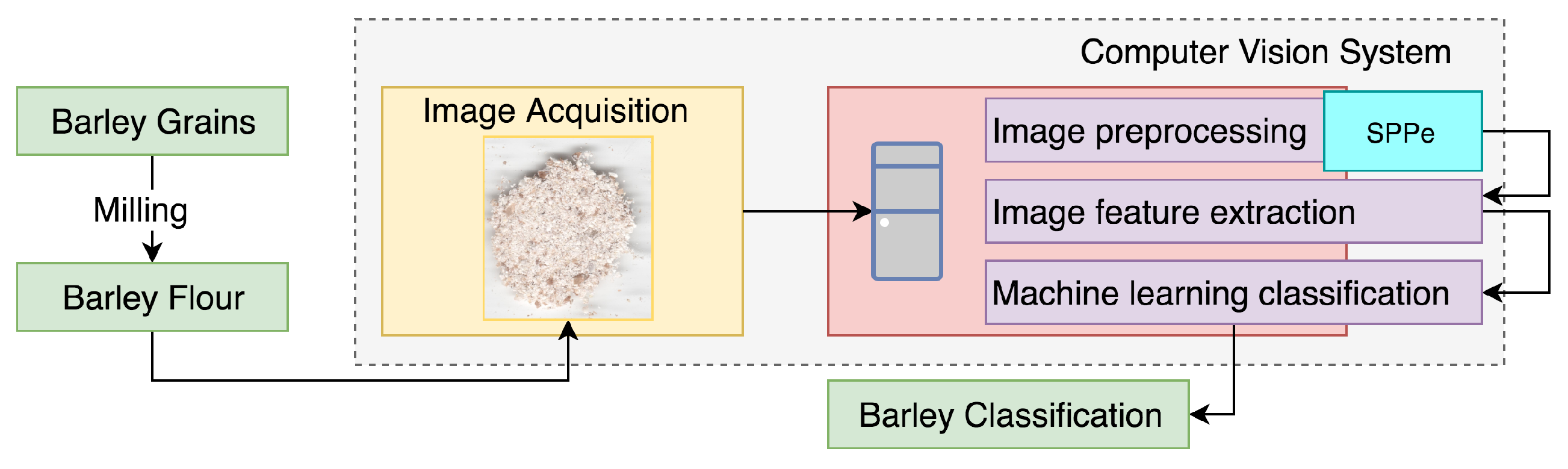
3.1. Computer Vision System

The CVS was constructed to classify samples as malting or naked barley, through the analysis of barley flour images. The employed CVS can be detailed as four main steps: acquisition, preprocessing, feature extraction, and classification (Figure 2).
It is important to highlight that the proposed SPPe is a technique to improve the classification performance grounded on a more informative strategy from the image sample before image feature extraction. SPPe requires interactive production of sub-images from an original sample image. These new sub-images had features extracted for enriching the dataset with complementary sources of information. Prediction of the original sample was based on a voting process for the sub-image samples’ classification, as detailed in Section 3.2.

Image Acquisition and Preprocessing

The samples were collected from two different types for creating the image dataset: malting barley B and naked barley N (Figure 3).
Images (1200 dpi) were acquired by a computer vision system where each individual barley flour portion was scanned (HP Laser Jet M1120 MFP, Hewlett-Packard, Louveira, Brazil), using image acquisition software (HP Precision Scan Pro, Version 6 . 1 , 2009). The images were acquired (14,028 × 10,208 pixels) and stored as a .jpg file for further processing, as described in Section 3.2.1. A total of 110 barley sample images were collected, five from each cultivar, 40 from naked barley and 70 from malting barley. The ROI was cropped from the original image considering the largest square in individual portion of barley flour, removing the background and contour of each sample.
The main goal of preprocessing was background removal, keeping the ROI. To achieve this, the image was converted to the monochromatic space channel, and the background was removed using image thresholding. This threshold value was selected using Otsu’s thresholding since it is one of the most widely-used methods for image segmentation. Since this image thresholding may lead to the removal of some pixels of the ROI, all the holes in the barley flour area were filled using a connectivity approach. At this point, the obtained image mask (representing the foreground) was used to find the center of mass of the object (barley flour samples). As the final step, the center of the mask found was used to grow a predefined square until reaching the object edge. The square mask was applied on to the original image, cropping the ROI.

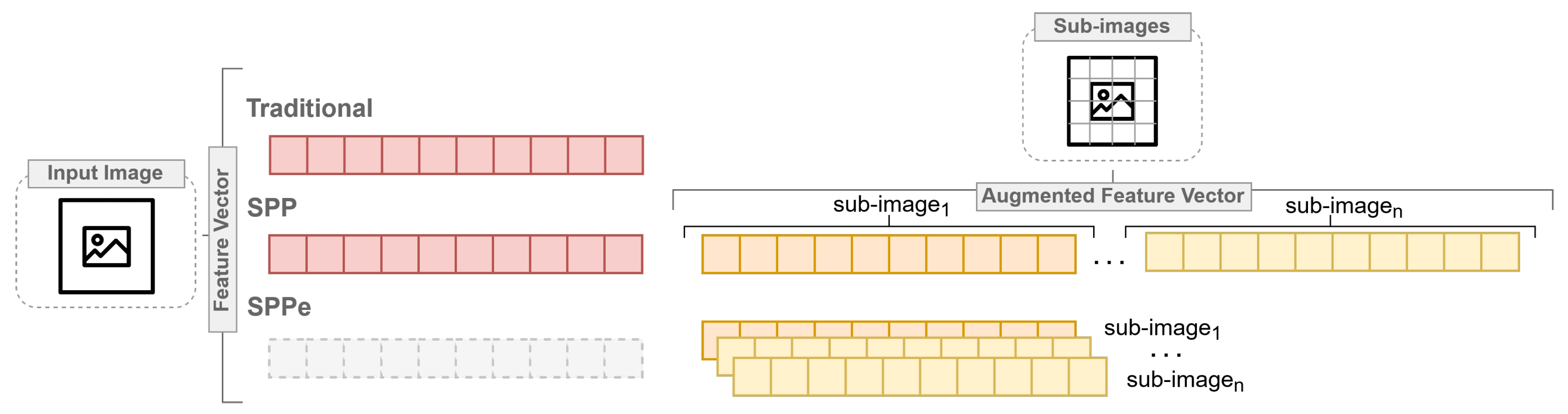
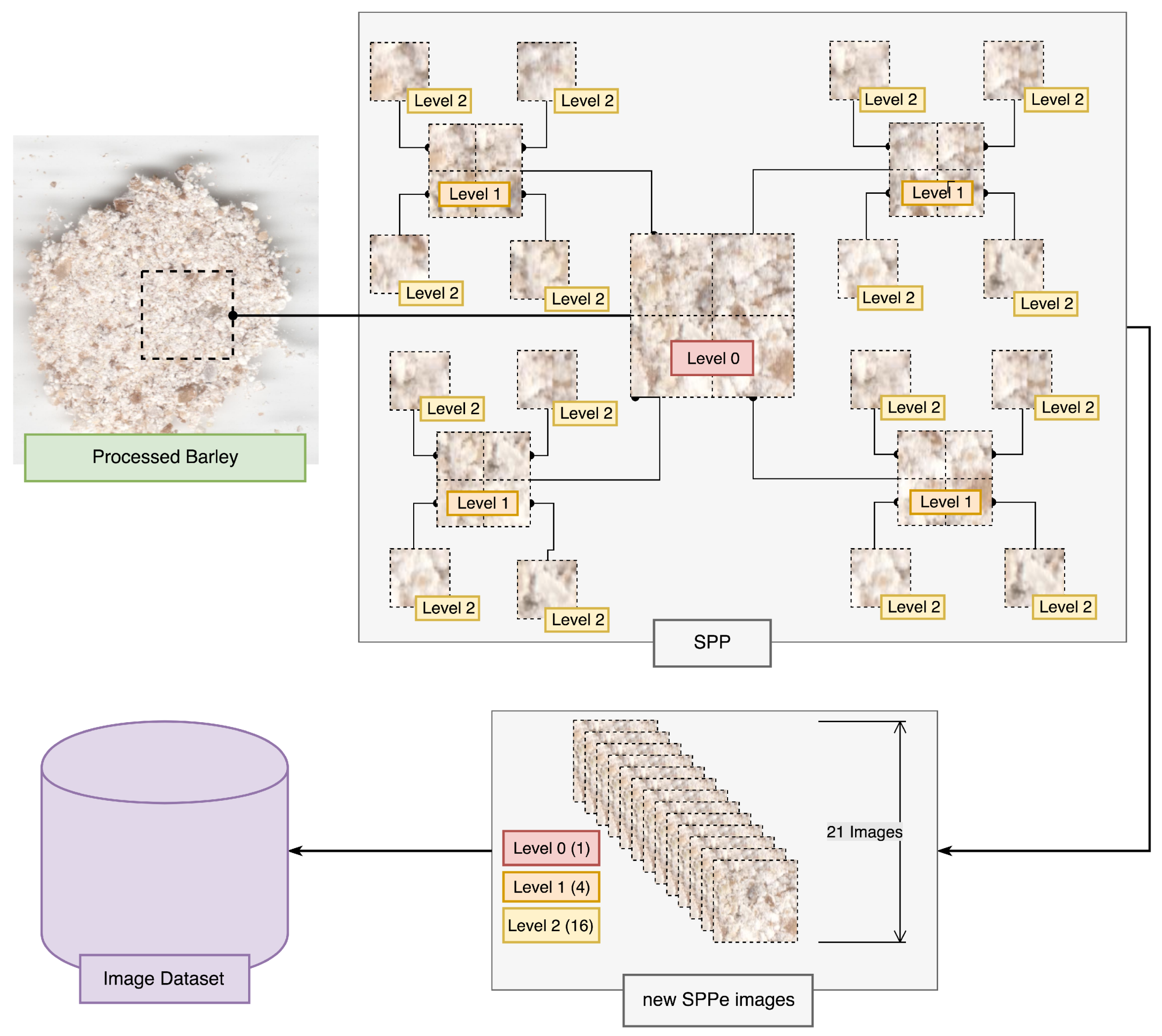
3.2. Spatial Pyramid Partition Ensemble

In the current work, we propose SPPe as part of the preprocessing step (Figure 2), to obtain a complete pattern comprehension of each sample. Our technique is a modification of the traditional SPP proposed in Sharma et al. [21]. Spatial Pyramid Partition (SPP) is based on splitting each image into a sequence of smaller sub-regions, extracting local image features from each image, and encoding their features into a vector [43,44]. In this sense, a given image is viewed as its low-level visual features extracted from all sub-regions. Each image is split into three levels, Level 0 being the image of the ROI by removing edges; Level 1 subdivides the ROI into four distinct parts, extracting its features; Level 2 subdivides each of the previous partitions into four other partitions, totaling 21 images from each ROI for extracting features to fine-tune the dataset. As a result, high-level and low-level features are extracted from the SPP image sequence to compose the image feature vector [21].
The proposed SPPe adapted the original SPP using an ensemble strategy to obtain the image classification. As opposed to traditional SPP, the aggregated image feature vector was not comprised of all sub-region, as a bag of features. Figure 4 presents an overview of the SPPe approach of creating sub-regions. Considering the description of image splitting, a new dataset was formed, which was composed of the sub-regions designated as Level 1 and 2. Thus, a feature vector was built from each sub-region without concatenating all regions. The ensemble strategy was applied to modify the dataset samples made up of smaller regions (Figure 4). Therefore, the sub-regions were used for problem modeling. After the prediction of a given sample from each sub-region, the scheme applied a weighing vote. In other words, we employed SPP with a subdivision strategy, to classify the Level 0 samples, and we considered each image separately for classification. Following the sub-regions’ prediction, we aggregated them with the respective sample to analyze as Level 0. In this way, from a new sample image, each sub-region obtained from SPPe was classified, and the final decision was achieved by a voting step.
A single model was induced for predicting all sub-regions from different levels. The induction of the classification model was carried out in the Leave-One-Subject-Out (LOSO) scheme to avoid bias [45]. The method employed the LOSO procedure to bind the sub-regions and their image Level 0, keeping all of them together in the training or test phase. In other words, each sub-image was bound to the respective sample (Level 0) and received its label. Hence, the sub-regions were considered non-independent regions as part of the same sample. This methodology guarantees the model learns nothing about the subject to be predicted. Thereby, the technique to be applied decreases the learning bias, achieving accurate results.
The SPPe output is based on the relation between the number of correct and incorrect sub-regions classified toward a majority decision as an ensemble prediction. Each level of partition by the SPPe method was assigned a voting weight. In the proposed experiment, for Level 1, it was assigned a weight of 1 / 3 and for Level 2, 1 / 12 for each ensemble member (image prediction). At the end of the iterations, the final result was computed considering each vote multiplied by the assigned weight. The final classification was obtained as the majority weighted vote from 20 sub-regions (4 from Level 1 and 16 from Level 2). This procedure creates a more reliable source of image classification by reducing overfitting, providing a robust description of barley based on several regions and dimensions.
We performed the original SPP proposed by Sharma et al. [21] in order to compare the SPPe performance improvements. SPPe avoids the high dimensional drawback, as in our scenario, SPP demands a total of 1155 image features per sample, while SPPe maintains only 55, both using only one classification model. Another important factor is related to the presence of visual components (e.g., husks) that could lead to noisy or biased features in the image description vector. Using an ensemble technique such as SPPe, we could reduce the overfitting of the final model [33], since the visually undesired components are lost in the final decision by a minority vote.
Each image obtained from the SPPe method had its features extracted independently of the level by the same descriptors for further analysis (as described in Section 3.2.1).

3.2.1. Image Analysis and Feature Extraction

Step 2 is related to the image feature extraction in a sequence of previous procedures (Figure 2). The extracted features are groups of discriminatory properties suitable to distinguish the classes between naked and malting samples. We extracted a set of 55 image features based on color, intensity, and texture. The list including all image features used in our solution is presented in Table 2.
Concerning color descriptors, statistical moments from the CIE L*a*b* and HSV color spaces were used, similarly to Li et al. [43] and Campos et al. [46]. The image acquired was stored in the RGB format, where each pixel is based on three color space: R (red), G (green), and B (blue). Due to the brightness information presented in the whole color channel from RGB, a good practice is related to selecting a different color space able to isolate brightness. For this reason, the transformation of input images from RGB to CIE L*a*b and HSV was considered toward extracting color features. The CIE L*a*b* and HSV color spaces were explored in this study: L* (Lightness), a* (red-green), b* (yellow-blue), Hue (H), Saturation (S), and Value (V) color channels, respectively. The mean and standard deviation were calculated for each color channel. Moreover, we computed the standard deviation, kurtosis, and skewness from the histogram of each channel, comprising a total of 30 color features.
Likewise, the same five statistical moments were used to describe the intensity information of each image. The pixel intensity was calculated from the average of RGB values. Image entropy, which can be characterized as a statistical measure of the randomness, texture, and contrast of grey scale images, was calculated for the intensity channel [47].
Both color and intensity variations between samples can be observed in Figure 3. Therefore, those features were used to properly describe the samples, allowing the machine learning algorithms to find the correct relations between features and barley types.
The texture is an important feature to identify objects or the presence of patterns in an image [48]. In this case, texture features were used to distinguish between different types of barley. For example, the presence of husk fragments in milled barley affects some features and could characterize a specific type of barley flour. Thus, having general applicability, three texture descriptors were used: Local binary patterns [49], Grey Level Co-occurrence Matrix (GLCM) [48], for which distance d = 1 and angle 0 considering 256 grey levels, and Fast Fourier Transform (FFT), this last to uncover frequency domain characteristics [50,51].
It is important to mention that we selected some traditional image descriptors to compose our feature vector, leveraging the comparison among the approaches for barley flour classification. Nevertheless, different image classification tasks can take more advantage of SPPe by employing alternative image features, e.g., features grounded on discrete wavelet transform [52] or fractal dimension [53].

3.2.2. Machine Learning

Features extracted from images are often used for classification and regression models, in order to identify samples from different classes or to predict quality parameters. In this way, machine learning algorithms can induce models from image features for automatic classification of barley flour. The modeling complexity of a machine learning system can vary greatly, allowing a high degree of customized freedom with appropriate trade-offs inherent in each specific scenario [54]. Some of the approaches include linear methods and non-linear machine learning algorithms, such as k-nearest neighbor, support vector machine, J48 decision tree, and random forest [46].
A brief description of the algorithms and the corresponding packages used to implement each ML algorithm are described in Table 3. In our experiments, the hyperparameters used were the default values of Rpackages in order to support a fair comparison among the algorithms.
In our experiment, the algorithms were applied in the R environment to induce models for barley flour classification. In order to achieve a reliable evaluation, two datasets were created: cross-validation and prediction test set. The cross-validation set was used to induce the models, adjusting the hyperparameters 10-fold considering 1800 images (Levels 1 and 2), while the prediction set was employed to test the classification performance using 400 images (Levels 1 and 2). Separation of samples into training and test sets was made in order to minimize the risks of overfitting, using the Kennard–Stone algorithm [60]. It is important to mention that the samples were split into the training and testing set considering Level 0 (a group of sub-regions), 90 samples (81.8%) for training and 20 samples (18.2%) for testing.

3.3. Evaluation Metrics

Performance evaluation of the models from machine learning was done using the total accuracy method (accuracy matrix) [61]. It is computed through the confusion matrix, which is defined by Equation (1).
T o t a l A c c u r a c y = T P + T N n
The total accuracy is calculated by the sum of the main diagonal values from the confusion matrix. These values are the True Positive (TP) and True Negative (TN), which are divided by the sum of the values from the whole matrix (n). Thus, it is possible to compute the performance of the image features and machine learning algorithms through the relation of the correctly-classified samples of barley flour. Recall (Equation (2)) and precision (Equation (3)) are often used to evaluate the effectiveness of classification methods based on False Negatives (FN) and False Positives (FP). In our work, we employed these metrics in order to support a fair comparison of the methods’ quality.
R e c a l l = T P T P + F N
P r e c i s i o n = T P T P + F P
Additionally, processing time from feature extraction to prediction was compared. Thus, it is possible to estimate overall job execution with an additional perspective of performance analysis. In the experiments, the time cost was calculated as the average of 30 runs. Dealing with descriptors, random forest importance was applied to this approach. The RF algorithm estimates the importance of a variable being observed when the prediction error increases if data for that variable are permuted, while all others are left unchanged. Based on the trees, as the random forest is constructed, RF’s importance investigates each extracted image feature, measuring the impact of characteristic samples in order to predict them [33].
In order to evaluate features extracted from barley flour samples, the exposed metric of variable importance demonstrates the advantage of random forest permutation because it embraces the impact of each predictor variable individually, as well as in multivariate interactions with other predictor variables.

4. Results and Discussion

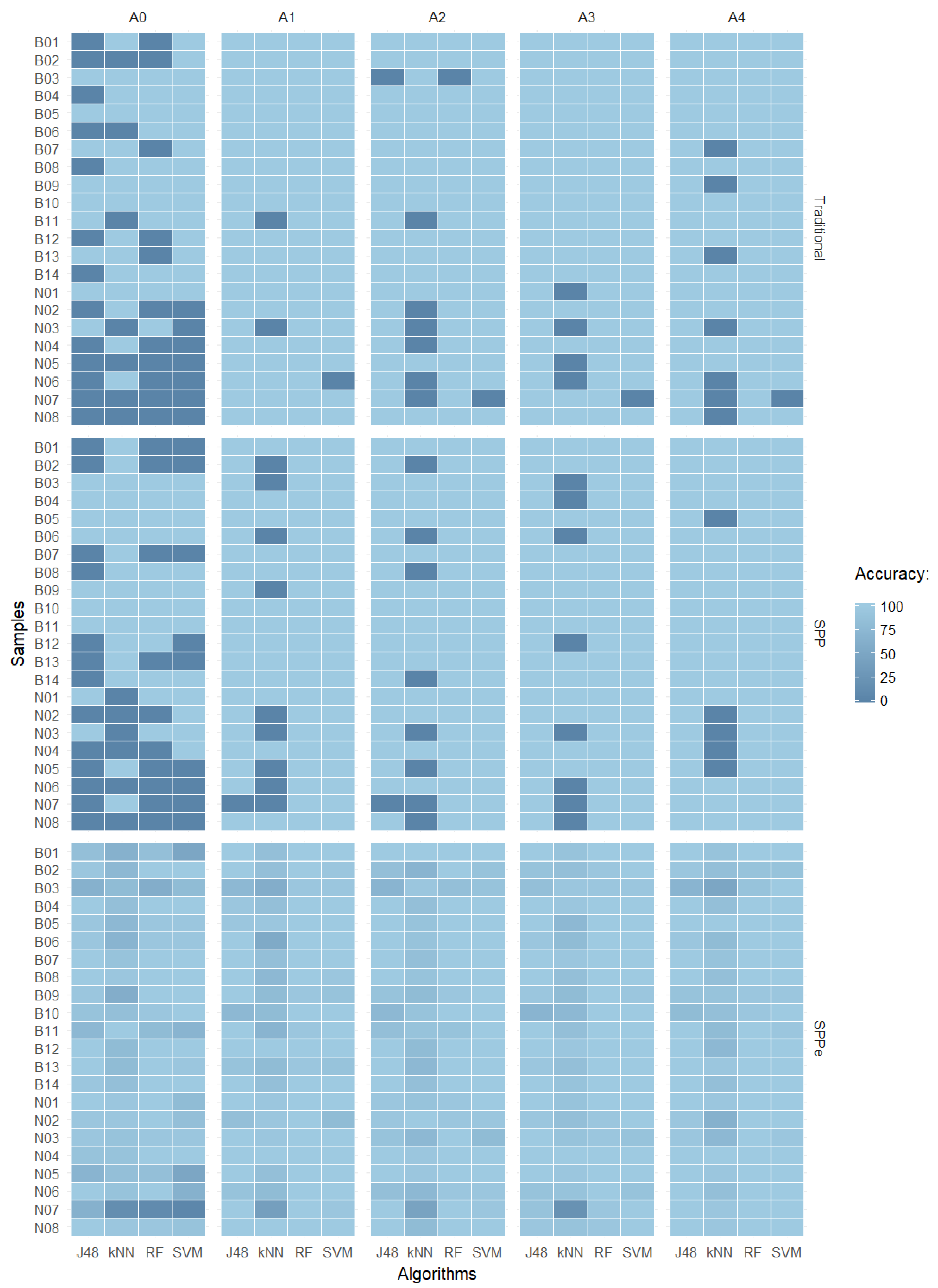
4.1. Algorithms and Image Processing Methods

The results of algorithm performance for the classification of naked and malting barley flour revealed the advantages of the proposed SPPe method, in comparison to SPP and traditional approaches. The experiments showed distinct performance values achieved with the techniques applied to this approach using machine learning algorithms. In order to establish a practical performance testing environment, the experiments were executed with Intel®Core i7-6700 CPU 3.40 GHz 16 GB memory. Table 4 summarizes the results obtained for prediction algorithms over the datasets considering performance measures such as: accuracy, precision, recall, and average processing time.
Comparing the machine learning algorithms, k-NN provided the worst performance, with accuracy values equal to or below 80 . 00 % for prediction using all methods investigated. Concerning only the results of the traditional CVS approach, (without SPP or SPPe) for the prediction set, RF obtained superior performance, with 90 . 00 % of accuracy and precision/recall values of 86 . 67 % , while SVM and k-NN presented similar accuracy ( 80 . 00 % ).
The original SPP presented superior results compared to the traditional method. SVM ( 92 . 00 % ) and RF ( 91 . 00 % ) reached superior results compared to J48 ( 88 . 00 % ) and k-NN ( 70 . 56 % ) for accuracy considering the cross-validation set. For the prediction set, RF obtained superior results, similar to SVM ( 95 . 00 % ). The worst metrics evaluated for the prediction set using the SPP technique was k-NN ( 60 . 00 % ), followed by J48 ( 85 . 00 % ).
An improvement of classification accuracy was obtained by SPPe technique with ML algorithms (Table 4). The average performance of classification considering all machine learning algorithms was improved from 83 . 75 % in the traditional method and original SPP to 91 . 25 % in accuracy for prediction sets. It is important to highlight that J48 stood out with 100 % accuracy, and k-NN maintained the lowest performance with 95 . 56 % (cross-validation set) and 75 . 00 % (prediction set). Likewise, the SPPe solution had the lowest processing time cost in comparison to SPP. Furthermore, traditional CVS provided better results than SPPe using k-NN.
Considering the processing time of the applied methods, CVS spent less time, being faster than SPP and SPPe, as expected. When comparing SPP and SPPe, our proposal was faster than SPP in all experiments. It is clear that the time cost tends to enlarge when the feature vector expands, as proposed by SPP and SPPe; however, the trade-off between predictive performance and processing time suggests the SPPe as a suitable solution when the main goal is the classification performance.

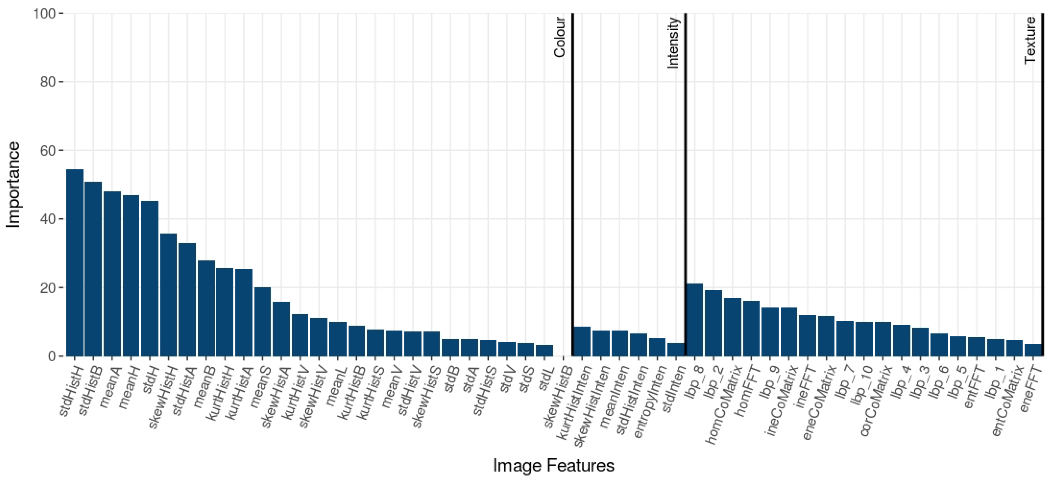
4.2. Evaluation of Image Features

The RF importance exposes the most relevant features in prediction tasks. The importance values are summarized in Figure 5. The most important features were from color: standard deviation values of the H and b* channels histogram (hue from HSV and yellow-blue CIE L*a*b* color spaces) were the most relevant explaining features with more scores higher than 50. Several statistic values from H, B*, and a* overcame texture and intensity features, although all features presented an impact for the classification procedure.
In order to characterize the types of barley flour, the mean and standard deviation of the grey-scale image, and hue HSV channel were the most discriminative image features. Moreover, the values of a* and b* channels gained higher importance, as well as the saturation. Texture features were significant for predicting the samples. Indeed, some texture features of the grey level co-occurrence matrix, and some LBP metrics were efficient at predicting variations of samples and also could be related to the granularity present in the barley flour.
Figure 6 summarizes the results in which it is possible to observe some misclassified samples by comparing all performed techniques with five different repetitions of acquisition (A0, A1, A2, A3, and A4). Correctly-classified samples are presented in light blue, while dark blue shows the misclassified samples for each method. It is possible to observe that the naked class presented more misclassified samples, meaning it is more complex to predict. For some classification algorithms, it is possible to observe similar behaviors among the samples, with k-NN as the worst performance.
Analyzing the misclassified samples, it was possible to identify similar patterns in both naked and malting types. Observing the accuracy error, it is possible to conclude that naked sample N07 ( 37 % error) presented similar characteristics to malting samples. Figure 7 presents an overview of the N07 cultivar, where it is possible to observe details by comparing the five samples as previously mentioned, and highlighted in the heat map shown in Figure 6. One possible explanation for the high error rate observed is the fact that Brazilian naked varieties were developed by using malting barley genes, so the studied features can be similar to those of malting barley varieties due to genetic origins [62].
Overall, SPPe demonstrated superior prediction ability compared to other methods, in addition to reduced overfitting and decreasing the high dimensionality present on the original SPP. Differences in composition/physical characteristics between the two barley groups (from naked and malting barley) were detected by the computer vision system, and classification accuracy was improved using SPPe.

4.3. SPPe in the Industry

There is an expressive advance when using the SPPe technique in comparison to the traditional CVS and SPP. The best result in the prediction set referred to J48 predictive performance and with low processing time in comparison to SPP. The proposed vision system was designed for an embedded process to provide high-level information for the barley flour industry environment. The system can be implemented by three sub-division steps:
  • The input image (acquisition) being extracted from the camera. Images are acquired by a camera placed at the scene under inspection.
  • The scene has to be appropriately illuminated and arranged, which promotes suitable reception of the image properties that are necessary for image processing (feature extraction and classification).
  • The processing system stage consists of a computer employed for processing the acquired images, resulting in classifying as naked or malting barley flour.
Combining the embedded technology with image processing, a future application in barley flour recognition types for quality control industry is possible.
Our proposal is a viable solution for barley flour industrial processing, as well as similar flour food products. More specifically, our proposal contributes to the industry in different stages of production. The CVS can be used as a quality control, observing specific supplier and providing financial advantages for high-quality flour. The proposed solution can be integrated into processing lines to identify barley according to the application, i.e., whether it is destined for infant formula, health food, and the malting industry, among other industrial production. It is important to highlight that the SPPe was fashioned with a minor feature vector in comparison with the SPP technique, spending less time to process, being faster and promoting its implementation in the production line.

5. Conclusions

This work proposed a system based on ML algorithms and computer vision developed to solve the automatic data analysis. A new proposed approach of Spatial Pyramid Partition ensemble (SPPe) provided better results for classification of barley flour into two different classes when compared to Spatial Pyramid Partition (SPP) and traditional CVS. Differences in barley composition cause variation of the flour’s physical characteristics, which were detected by image analysis. The proposed method showed a significant improvement, by reducing overfitting, avoiding dimensional growth, and improving classification accuracy for several machine learning algorithms. The importance of all image descriptors (color, intensity, and texture) for providing helpful information to distinguish between malting and naked barley flour samples was identified. The best model was built using the SPPe with J48 decision tree, allowing the classification of 100% of samples. The results of this study are promising, and they could allow the development of an effective model in order to expand its use in the food industry, reducing costs and improving the effectiveness of automatic quality inspection.

Author Contributions

Conceptualization, M.V.E.G. and S.B.J.; Methodology, J.F.L.; Software, S.B.J.; Validation, J.F.L., L.L. and S.B.J.; Formal analysis, J.F.L.; Investigation, D.F.B.; Resources, L.L.; Data curation, L.L.; Writing–original draft preparation, S.B.J.; Writing–review and editing, J.F.L., L.L, D.F.B., M.V.E.G. and S.B.J.; Visualization, J.F.L.; Supervision, S.B.J.; Project administration, J.F.L.; Funding acquisition, S.B.J.

Funding

This work has been partially supported by the National Council for Scientific and Technological Development (CNPq) of Brazil under a grant of Project 420562/2018-4.

Acknowledgments

The authors would like to thank CAPES for financial support.

Conflicts of Interest

The authors declare no conflict of interest.

References

  1. Idehen, E.; Tang, Y.; Sang, S. Bioactive phytochemicals in barley. J. Food Drug Anal. 2017, 25, 148–161. [Google Scholar] [CrossRef]
  2. Bhatty, R. β-Glucan content and viscosities of barleys and their roller-milled flour and bran products. Cereal Chem. 1992, 69, 469–471. [Google Scholar]
  3. Taketa, S.; Kikuchi, S.; Awayama, T.; Yamamoto, S.; Ichii, M.; Kawasaki, S. Monophyletic origin of naked barley inferred from molecular analyses of a marker closely linked to the naked caryopsis gene (nud). Theor. Appl. Genet. 2004, 108, 1236–1242. [Google Scholar] [CrossRef]
  4. Edney, M.J.; O’Donovan, J.T.; Turkington, T.K.; Clayton, G.W.; McKenzie, R.; Juskiw, P.; Lafond, G.P. Effects of seeding rate, nitrogen rate and cultivar on barley malt quality. Sci. Food Agric. 2015, 92, 2672–2678. [Google Scholar] [CrossRef]
  5. Shewry, P.R.; Ullrich, S.E. Barley: Chemistry and Technology; AACCI Press: St. Paul, MN, USA, 2014; Volume 2. [Google Scholar]
  6. Paredes, P.; Rodrigues, G.C.; do Rosário Cameira, M.; Torres, M.O.; Pereira, L.S. Assessing yield, water productivity and farm economic returns of malt barley as influenced by the sowing dates and supplemental irrigation. Agric. Water Manag. 2017, 179, 132–143. [Google Scholar] [CrossRef]
  7. Lim, J.; Kim, G.; Mo, C.; Oh, K.; Kim, G.; Ham, H.; Kim, S.; Kim, M. Application of near infrared reflectance spectroscopy for rapid and non-destructive discrimination of hulled barley, naked barley, and wheat contaminated with Fusarium. Sensors 2018, 18, 113. [Google Scholar] [CrossRef]
  8. Newman, C.W.; Newman, R.K. A brief history of barley foods. Cereal Foods World 2006, 51, 4–7. [Google Scholar] [CrossRef]
  9. Szczypinski, P.M.; Klepaczko, A.; Zapotoczny, P. Identifying barley varieties by computer vision. Comput. Electron. Agric. 2015, 110, 1–8. [Google Scholar] [CrossRef]
  10. Du, C.J.; Sun, D.W. Learning techniques used in computer vision for food quality evaluation: A review. J. Food Eng. 2006, 72, 39–55. [Google Scholar] [CrossRef]
  11. Kurtulmuş, F.; Gürbüz, O.; Değirmencioğlu, N. Discriminating drying method of tarhana using computer vision. J. Food Process Eng. 2014, 37, 362–374. [Google Scholar] [CrossRef]
  12. Patrício, D.I.; Rieder, R. Computer vision and artificial intelligence in precision agriculture for grain crops: A systematic review. Comput. Electron. Agric. 2018, 153, 69–81. [Google Scholar] [CrossRef] [Green Version]
  13. Sabanci, K.; Kayabasi, A.; Toktas, A. Computer vision-based method for classification of wheat grains using artificial neural network. Sci. Food Agric. 2016, 97, 2588–2593. [Google Scholar] [CrossRef]
  14. Aslan, M.F.; Sabanci, K.; Yiğit, E.; Kayabaşi, A.; Toktaş, A.; Duysak, H. A Comparative Classification of Wheat Grains for Artificial Neural Network and Extreme Learning Machine. Uluslararası Çevresel Eğilimler Derg. 2017, 1, 14–21. [Google Scholar]
  15. Mittal, G.S. Computerized Control Systems in the Food Industry; Marcel Dekker, Inc.: New York, NY, USA, 1996. [Google Scholar]
  16. Zhao, X.; Wang, W.; Ni, X.; Chu, X.; Li, Y.F.; Sun, C. Evaluation of Near-infrared hyperspectral imaging for detection of peanut and walnut powders in whole wheat flour. Appl. Sci. 2018, 8, 1076. [Google Scholar] [CrossRef]
  17. Lohumi, S.; Lee, H.; Kim, M.S.; Qin, J.; Kandpal, L.M.; Bae, H.; Rahman, A.; Cho, B.K. Calibration and testing of a Raman hyperspectral imaging system to reveal powdered food adulteration. PLoS ONE 2018, 13, e0195253. [Google Scholar] [CrossRef]
  18. Foca, G.; Masino, F.; Antonelli, A.; Ulrici, A. Prediction of compositional and sensory characteristics using RGB digital images and multivariate calibration techniques. Anal. Chim. Acta 2011, 706, 238–245. [Google Scholar] [CrossRef]
  19. Su, W.H.; Sun, D.W. Fourier transform infrared and Raman and hyperspectral imaging techniques for quality determinations of powdery foods: A review. Compr. Rev. Food Sci. Food Saf. 2018, 17, 104–122. [Google Scholar] [CrossRef]
  20. Xu, Y.; Yu, X.; Wang, T.; Lu, F. Discriminative Spatial Tree for Image Classification. In Proceedings of the 2017 IEEE International Conference on Smart Cloud (SmartCloud), New York, NY, USA, 3–5 November 2017; pp. 283–288. [Google Scholar]
  21. Sharma, G.; Jurie, F.; Schmid, C. Discriminative spatial saliency for image classification. In Proceedings of the 2012 IEEE Conference on Computer Vision and Pattern Recognition (CVPR), Providence, RI, USA, 16–21 June 2012; pp. 3506–3513. [Google Scholar]
  22. Pereira, L.F.S.; Barbon, S.; Valous, N.A.; Barbin, D.F. Predicting the ripening of papaya fruit with digital imaging and random forests. Comput. Electron. Agric. 2018, 145, 76–82. [Google Scholar] [CrossRef]
  23. Da Costa Barbon, A.P.A.; Barbon, S., Jr.; Campos, G.F.C.; Seixas, J.L.S., Jr.; Peres, L.M.; Mastelini, S.M.; Andreo, N.; Ulrici, A.; Bridi, A.M. Development of a flexible Computer Vision System for marbling classification. Comput. Electron. Agric. 2017, 142, 536–544. [Google Scholar] [CrossRef]
  24. Kurtulmuş, F.; Ünal, H. Discriminating rapeseed varieties using computer vision and machine learning. Expert Syst. Appl. 2015, 42, 1880–1891. [Google Scholar] [CrossRef]
  25. Wang, D.; Wang, X.; Liu, T.; Liu, Y. Prediction of total viable counts on chilled pork using an electronic nose combined with support vector machine. Meat Sci. 2012, 90, 373–377. [Google Scholar] [CrossRef] [PubMed]
  26. Liu, M.; Wang, M.; Wang, J.; Li, D. Comparison of random forest, support vector machine and back propagation neural network for electronic tongue data classification: Application to the recognition of orange beverage and Chinese vinegar. Sens. Actuators B Chem. 2013, 177, 970–980. [Google Scholar] [CrossRef]
  27. Papadopoulou, O.S.; Panagou, E.Z.; Mohareb, F.R.; Nychas, G.J.E. Sensory and microbiological quality assessment of beef fillets using a portable electronic nose in tandem with support vector machine analysis. Food Res. Int. 2013, 50, 241–249. [Google Scholar] [CrossRef]
  28. Prevolnik, M.; Andronikov, D.; Žlender, B.; Font-i Furnols, M.; Novič, M.; Škorjanc, D.; Čandek-Potokar, M. Classification of dry-cured hams according to the maturation time using near infrared spectra and artificial neural networks. Meat Sci. 2014, 96, 14–20. [Google Scholar] [CrossRef] [PubMed]
  29. Ai, F.F.; Bin, J.; Zhang, Z.M.; Huang, J.H.; Wang, J.B.; Liang, Y.Z.; Yu, L.; Yang, Z.Y. Application of random forests to select premium quality vegetable oils by their fatty acid composition. Food Chem. 2014, 143, 472–478. [Google Scholar] [CrossRef]
  30. Granitto, P.M.; Gasperi, F.; Biasioli, F.; Trainotti, E.; Furlanello, C. Modern data mining tools in descriptive sensory analysis: A case study with a Random forest approach. Food Qual. Prefer. 2007, 18, 681–689. [Google Scholar] [CrossRef]
  31. Barbon, A.P.A.; Barbon, S.; Mantovani, R.G.; Fuzyi, E.M.; Peres, L.M.; Bridi, A.M. Storage time prediction of pork by Computational Intelligence. Comput. Electron. Agric. 2016, 127, 368–375. [Google Scholar] [CrossRef]
  32. Liakos, K.; Busato, P.; Moshou, D.; Pearson, S.; Bochtis, D. Machine learning in agriculture: A review. Sensors 2018, 18, 2674. [Google Scholar] [CrossRef]
  33. Breiman, L. Random forests. Mach. Learn. 2001, 45, 5–32. [Google Scholar] [CrossRef]
  34. Vapnik, V.N. The Nature of Statistical Learning Theory; Springer-Verlag Inc.: New York, NY, USA, 1995. [Google Scholar]
  35. Brighton, H.; Mellish, C. Advances in Instance Selection for Instance-Based Learning Algorithms. Data Min. Knowl. Discov. 2002, 6, 153–172. [Google Scholar] [CrossRef]
  36. Hornik, K.; Karatzoglou, D.M.; Zeileis, A.; Hornik, M.K. The Rweka Package. 2007. Available online: ftp://ftp.uni-bayreuth.de/pub/math/statlib/R/CRAN/doc/packages/RWeka.pdf (accessed on 15 May 2019).
  37. Muñoz, I.; Rubio-Celorio, M.; Garcia-Gil, N.; Guàrdia, M.D.; Fulladosa, E. Computer image analysis as a tool for classifying marbling: A case study in dry-cured ham. J. Food Eng. 2015, 166, 148–155. [Google Scholar] [CrossRef]
  38. Saberioon, M.; Císař, P.; Labbé, L.; Souček, P.; Pelissier, P.; Kerneis, T. Comparative Performance Analysis of Support Vector Machine, Random Forest, Logistic Regression and k-Nearest Neighbours in Rainbow Trout (Oncorhynchus Mykiss) Classification Using Image-Based Features. Sensors 2018, 18, 1027. [Google Scholar] [CrossRef] [PubMed]
  39. Nowakowski, K.; Boniecki, P.; Tomczak, R.J.; Kujawa, S.; Raba, B. Identification of malting barley varieties using computer image analysis and artificial neural networks. In Proceedings of the Fourth International Conference on Digital Image Processing (ICDIP 2012), Kuala Lumpur, Malaysia, 7–8 April 2012; International Society for Optics and Photonics: San Diego, CA, USA, 2012; Volume 8334, p. 833425. [Google Scholar]
  40. Kociołek, M.; Szczypiński, P.M.; Klepaczko, A. Preprocessing of barley grain images for defect identification. In Proceedings of the 2017 IEEE Signal Processing: Algorithms, Architectures, Arrangements, and Applications (SPA), Poznan, Poland, 20–22 September 2017; pp. 365–370. [Google Scholar]
  41. Pazoki, A.; Pazoki, Z.; Sorkhilalehloo, B. Rain Fed Barley Seed Cultivars Identification Using Neural Network and Different Neurons Number. World Appl. Sci. J. 2013, 5, 755–762. [Google Scholar]
  42. Ciesielski, V.; Lam, B.; Nguyen, M.L. Comparison of evolutionary and conventional feature extraction methods for malt classification. In Proceedings of the 2012 IEEE Congress on Evolutionary Computation (CEC), Brisbane, QLD, Australia, 10–15 June 2012; pp. 1–7. [Google Scholar]
  43. Li, D.; Li, N.; Wang, J.; Zhu, T. Pornographic images recognition based on spatial pyramid partition and multi-instance ensemble learning. Knowl.-Based Syst. 2015, 84, 214–223. [Google Scholar] [CrossRef]
  44. Zhang, C.; Wang, S.; Huang, Q.; Liu, J.; Liang, C.; Tian, Q. Image classification using spatial pyramid robust sparse coding. Pattern Recognit. Lett. 2013, 34, 1046–1052. [Google Scholar] [CrossRef]
  45. Saez, Y.; Baldominos, A.; Isasi, P. A Comparison Sudy of Classifier Algorithms for Cross-Person Physical Activity Recognition. Sensors 2017, 17, 66. [Google Scholar] [CrossRef]
  46. Campos, G.F.; Barbon, S.; Mantovani, R.G. A meta-learning approach for recommendation of image segmentation algorithms. In Proceedings of the 2016 29th SIBGRAPI Conference on Graphics, Patterns and Images (SIBGRAPI), Sao Paulo, Brazil, 4–7 October 2016; pp. 370–377. [Google Scholar]
  47. Kapur, J.; Sahoo, P.; Wong, A. A new method for gray-level picture thresholding using the entropy of the histogram. Comput. Vis. Graph. Image Process. 1985, 29, 273–285. [Google Scholar] [CrossRef]
  48. Haralick, R.M.; Shanmugam, K.; Dinstein, I. Textural features for image classification. IEEE Trans. Syst. Man Cybern. 1973, 6, 610–621. [Google Scholar] [CrossRef]
  49. Ojala, T.; Pietikäinen, M.; Mäenpää, T. Multiresolution gray-scale and rotation invariant texture classification with local binary patterns. IEEE Trans. Pattern Anal. Mach. Intell. 2002, 24, 971–987. [Google Scholar] [CrossRef]
  50. Nixon, M.; Aguado, A.S. Feature Extraction and Image Processing for Computer Vision; Academic Press: Cambridge, MA, USA, 2012. [Google Scholar]
  51. Shen, H.K.; Chen, P.H.; Chang, L.M. Automated steel bridge coating rust defect recognition method based on color and texture feature. Autom. Constr. 2013, 31, 338–356. [Google Scholar] [CrossRef]
  52. Hiremath, P.; Shivashankar, S. Wavelet based co-occurrence histogram features for texture classification with an application to script identification in a document image. Pattern Recognit. Lett. 2008, 29, 1182–1189. [Google Scholar] [CrossRef]
  53. Chaudhuri, B.B.; Sarkar, N. Texture segmentation using fractal dimension. IEEE Trans. Pattern Anal. Mach. Intell. 1995, 17, 72–77. [Google Scholar] [CrossRef]
  54. Sutton, R.S. Learning to predict by the methods of temporal differences. Mach. Learn. 1988, 3, 9–44. [Google Scholar] [CrossRef]
  55. Cunningham, P.; Delany, S.J. k-Nearest neighbour classifiers. Mult. Classif. Syst. 2007, 34, 1–17. [Google Scholar]
  56. Quinlan, J. C4.5 Programs for Machine Learning; Morgan Kaufmann: San Mateo, CA, USA, 1992. [Google Scholar]
  57. Sharma, T.C.; Jain, M. WEKA approach for comparative study of classification algorithm. Int. J. Adv. Res. Comput. Commun. Eng. 2013, 2, 1925–1931. [Google Scholar]
  58. Scornet, E.; Biau, G.; Vert, J.P. Consistency of random forests. Ann. Stat. 2015, 43, 1716–1741. [Google Scholar] [CrossRef]
  59. Wang, L. Support Vector Machines: Theory and Applications; Springer Science & Business Media: New York, NY, USA, 2005; Volume 177. [Google Scholar]
  60. Kennard, R.W.; Stone, L.A. Computer aided design of experiments. Technometrics 1969, 11, 137–148. [Google Scholar] [CrossRef]
  61. Aggarwal, C.C. Data Classification: Algorithms and Applications; CRC Press: Boca Raton, FL, USA, 2014. [Google Scholar]
  62. Kroth, M.A.; Ramella, M.S.; Tagliari, C.; Francisco, A.D.; Arisi, A.C.M. Genetic Similarity of Brazilian Hull-Less and Malting Barley Varieties Evaluated by Rapd Markers. Agric. Sci. 2005, 62, 36–39. [Google Scholar] [CrossRef]
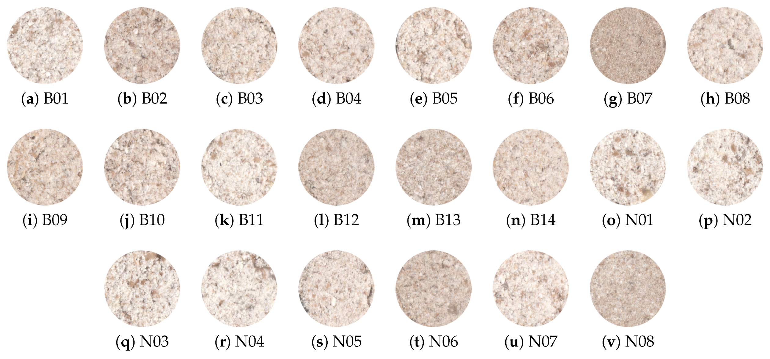
Figure 1. General overview highlighting the differences among traditional, SPP and Spatial Pyramid Partition ensemble (SPPe) approaches of feature vector composition.
Sensors 19 02953 g001
Figure 2. General overview of the proposed approach.
Sensors 19 02953 g002
Figure 3. Samples of barley flour from malting (an) and naked (ov) types.
Sensors 19 02953 g003
Figure 4. Spatial Pyramidal Partition ensemble (SPPe) for obtaining image samples.
Sensors 19 02953 g004
Figure 5. RF importance of image features.
Sensors 19 02953 g005
Figure 6. Accuracy heat map of J48, k-NN, RF, and SVM over the prediction dataset comparing traditional CVS, SPP, and SPPe techniques with repetitions A0, A1, A2, A3, and A4.
Sensors 19 02953 g006
Figure 7. Samples of cultivar N07, the lowest accuracy of barley flour classification.
Sensors 19 02953 g007
Table 1. Barley cultivars employed in the experimentation.B, malting Barley; N, Naked barley.
Sample IDCultivarType
B01BRS AliensaMalting
B02BRS ItanemaMalting
B03BRS BrauMalting
B04MN 6021Malting
B05BRS SampaMalting
B06BRS KorbelMalting
B07MN 6021Malting
B08BRS ElisMalting
B09BRS KorbelMalting
B10BRS ElisMalting
B11BRS ManduríMalting
B12BRS BrauMalting
B13BRS CauêMalting
B14BRS CauêMalting
N01149852Naked
N02149853Naked
N03149857Naked
N04149846Naked
N05149858Naked
N06149841Naked
N07149855Naked
N08149859Naked
Table 2. List of all image features used in the proposed SPPe approach for barley flour classification.
No.TypeNameDescription
1ColormeanHMean value of the H channel
2ColorStdHStandard deviation of the H channel
3ColormeanSMean value of the S channel
4ColorstdSStandard deviation of the S channel
5ColorMeanVMean value of the V channel
6ColorstdVStandard deviation of the V channel
7ColorstdHistHStandard deviation of H channel histogram
8ColorkurtHistHKurtosis of H channel histogram
9ColorskewHistHSkewness of H channel histogram
10ColorstdHistSStandard deviation of S channel histogram
11ColorkurtHistSKurtosis of S channel histogram
12ColorskewHistSSkewness of S channel histogram
13ColorstdHistVStandard deviation of V channel histogram
14ColorkurtHistVKurtosis of V channel histogram
15ColorskewHistVSkewness of V channel histogram
16ColormeanLMean value of the L channel
17ColorstdLStandard deviation of the L channel
18ColormeanAMean value of the A channel
19ColorstdAStandard deviation of the A channel
20ColormeanBMean value of the B channel
21ColorstdBStandard deviation of the B channel
22ColorstdHistLStandard deviation of L channel histogram
23ColorkurtHistLKurtosis of L channel histogram
24ColorskewHistLSkewness of L channel histogram
25ColorstdHistAStandard deviation of A channel histogram
26ColorkurtHistAKurtosis of A channel histogram
27ColorskewHistASkewness of A channel histogram
28ColorstdHistBStandard deviation of B channel histogram
29ColorkurtHistBKurtosis of B channel histogram
30ColorskewHistBSkewness of B channel histogram
31IntensitymeanIntenMean value of intensity image
32IntensityStdIntenStandard deviation of Intensity image
33IntensityentropyIntenEntropy of intensity image
34IntensitystdHistIntenStandard deviation of Intensity image histogram
35IntensitykurtHistIntenKurtosis of intensity image histogram
36IntensityskewHistIntenSkewness of intensity image histogram
37–46Texture l b p _ 0 - l b p _ 9 Vector of Local Binary Patterns (LBP) rotationally invariant features
47TextureentCoMatrixEntropy of grey-level co-occurrence matrix
48TextureineCoMatrixInertia of grey-level co-occurrence matrix
49TextureeneCoMatrixEnergy of grey-level co-occurrence matrix
50TexturecorCoMatrixCorrelation of grey-level co-occurrence matrix
51TexturehomCoMatrixHomogeneity of grey-level co-occurrence matrix
52TextureeneFFTFFT Energy
53TextureentFFTFFT Entropy
54TextureineFFTFFT Inertia
55TexturehomFFTFFT Homogeneity
Table 3. Machine learning algorithms used in the experiments and corresponding R packages.
AlgorithmDescriptionR PackageHyperparameters
K-Nearest Neighbor (k-NN)A non-parametric lazy learning algorithm; the training data are not used for any generalization [55].RWekaEuclidean distance; k= 5
Decision Tree (J48)A decision tree widely applied to represent series of rules that lead to a class or value [56,57].RWekaC = 0.25; threshold = 0.25; with pruning
Random Forest (RF)A combination of decision tree models that provides more accurate prediction [33,58].RandomForestntree = 100; mtry = 7
Support Vector Machine (SVM)A statistical learning algorithm, used for supervised ML and food quality solutions [34,59].e1071kernel = polynomial; γ = 0.02 , degree = 3
Table 4. Performance measures in the comparison of the methods and algorithms (RF, k-NN, J48 and SVM) over the cross-validation and prediction dataset.
AlgorithmMetricCross-ValidationPrediction
TraditionalSPPSPPeTraditionalSPPSPPe
RFAccuracy90.0091.00100.0090.0095.0095.00
Precision71.8871.88100.0086.6796.8896.88
Recall68.9369.43100.0086.6790.0090.00
Time (s)65.35 ( ± 0.13 )281.63 (±1.09)217.11 (±0.40)62.53 (±0.12)268.71 (±0.39)207.07 (±0.34)
k-NNAccuracy77.5670.5695.5680.0060.0075.00
Precision60.7957.2595.8574.5152.7565.63
Recall58.7953.8894.8166.6753.3363.33
Time (s)64.50 (±0.10)279.34 (±0.94)209.49 (±0.36)62.44 (±0.15)268.51 (±0.36)206.11 (±0.29)
J48Accuracy89.0088.00100.0085.0085.00100.00
Precision71.8871.88100.0079.7791.67100.00
Recall68.4367.93100.0083.3370.00100.00
Time (s)70.14 (±0.26)353.37 (±2.31)210.79 (±0.37)62.61 (±0.10)270.71 (±0.38)206.32 (±0.33)
SVMAccuracy93.0092.0098.8980.0095.0095.00
Precision70.4272.5099.1189.4796.8896.88
Recall70.0070.3698.5760.0090.0090.00
Time (s)64.62 (±0.15)280.57 (±0.95)213.40 (±0.43)62.83 (±0.12)268.66 (±0.37)206.75 (±0.37)

