On the Location of Fog Nodes in Fog-Cloud Infrastructures

Abstract
1. Introduction
2. Related work
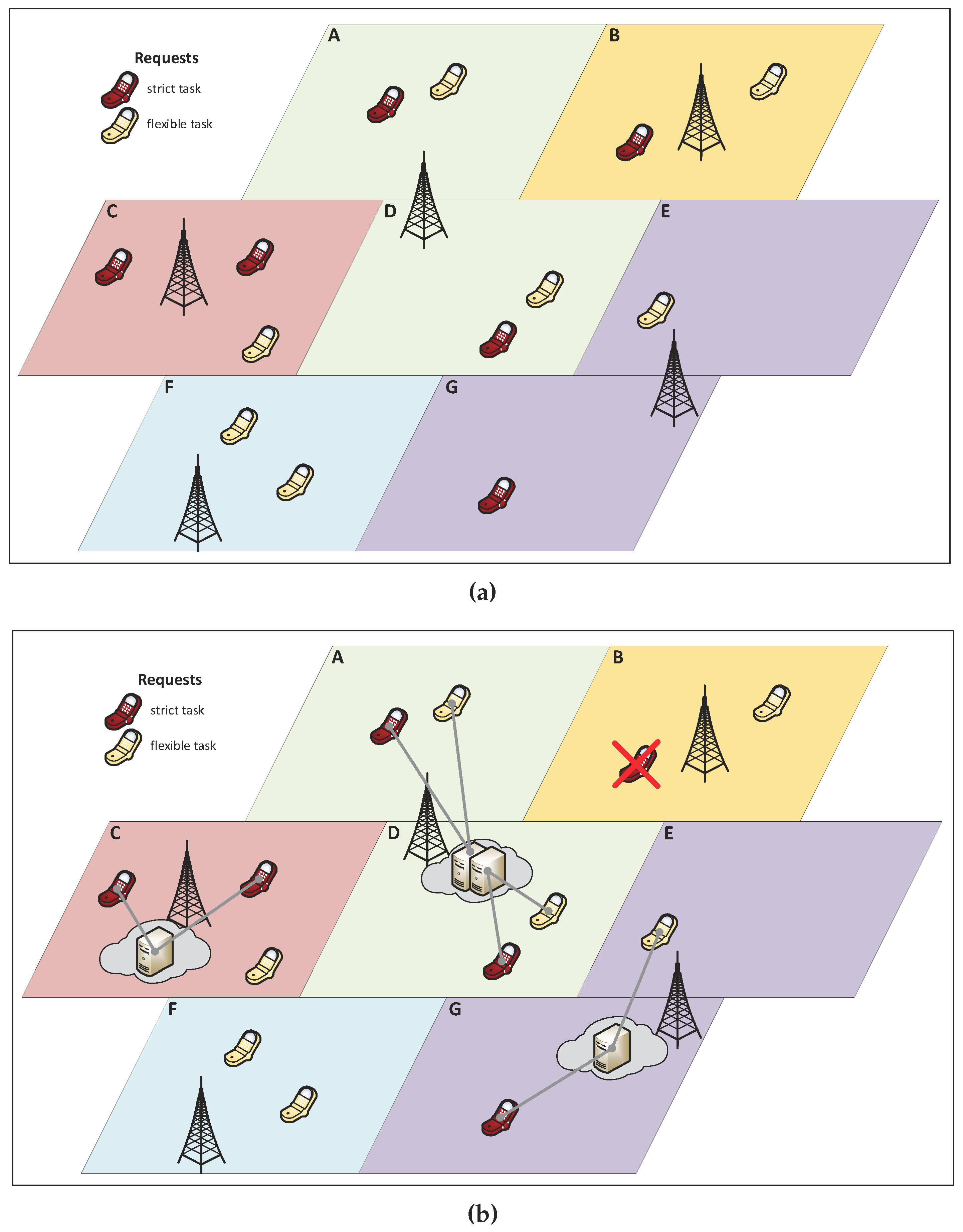
3. System Model
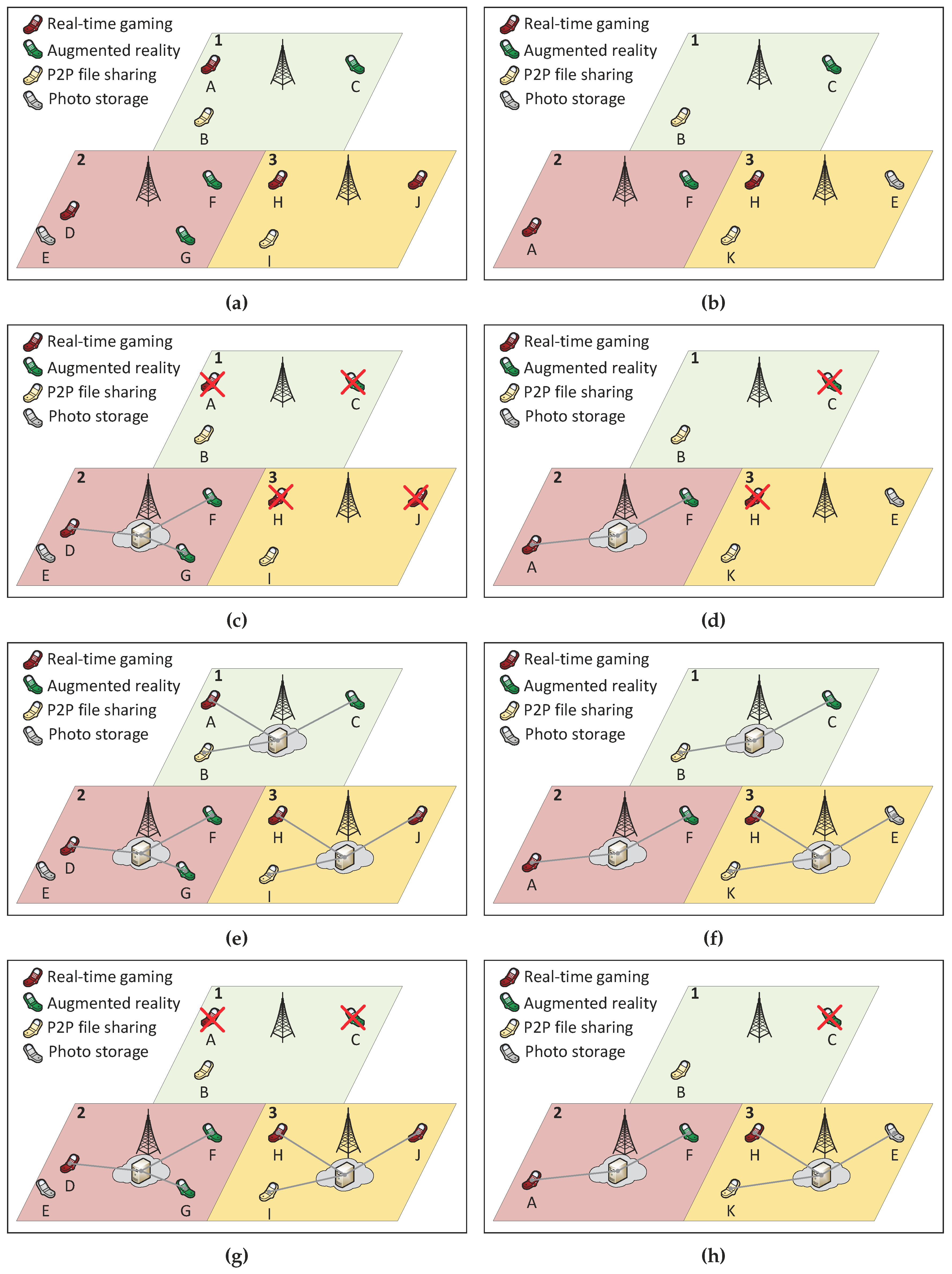
4. Fog Location Model
4.1. Mathematical Model
4.2. Multicriteria Decision
4.3. Numerical Example
5. Performance Evaluation
5.1. Workload
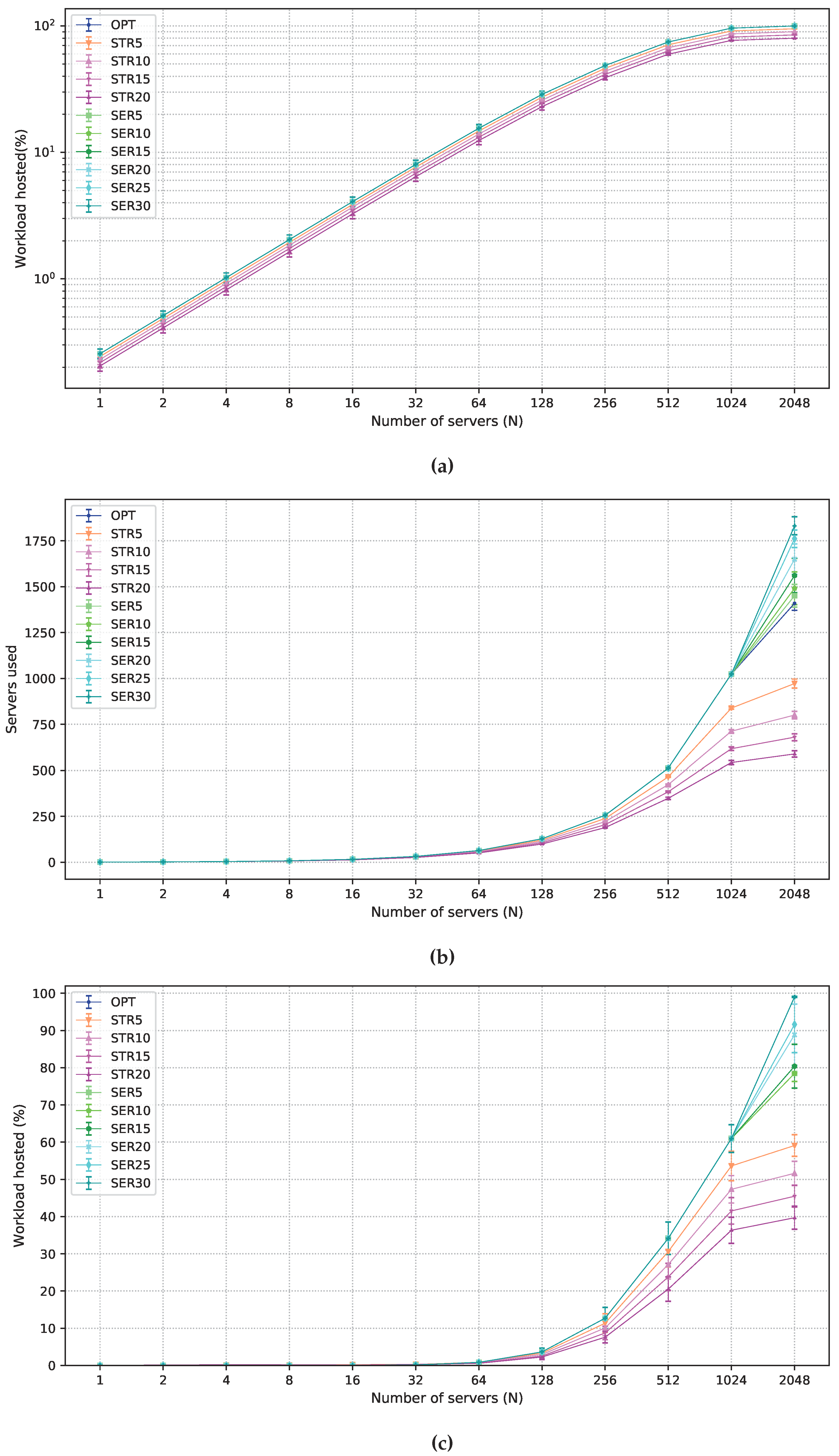
5.2. Multi-Objective Solutions Allowing Degradation
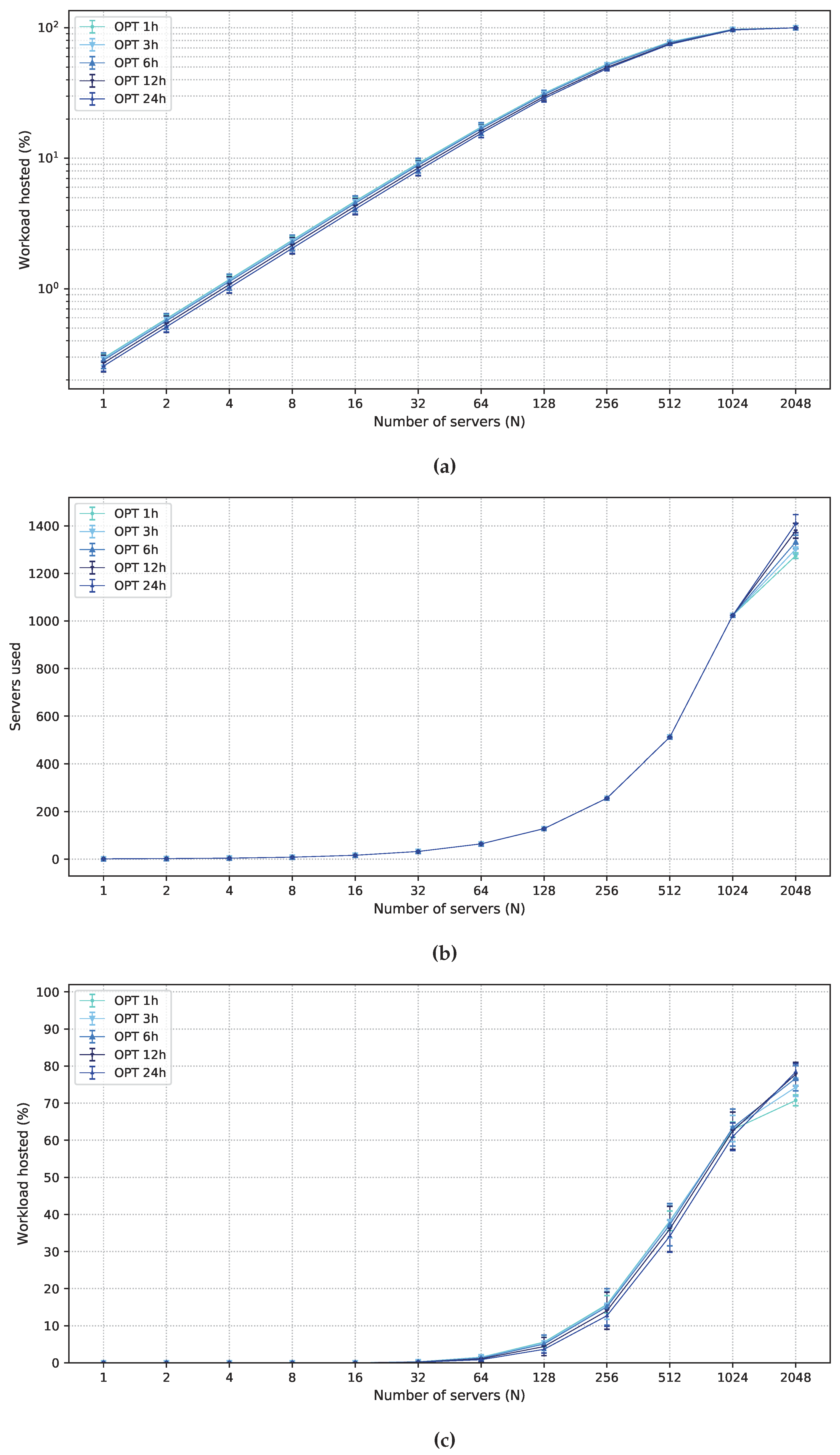
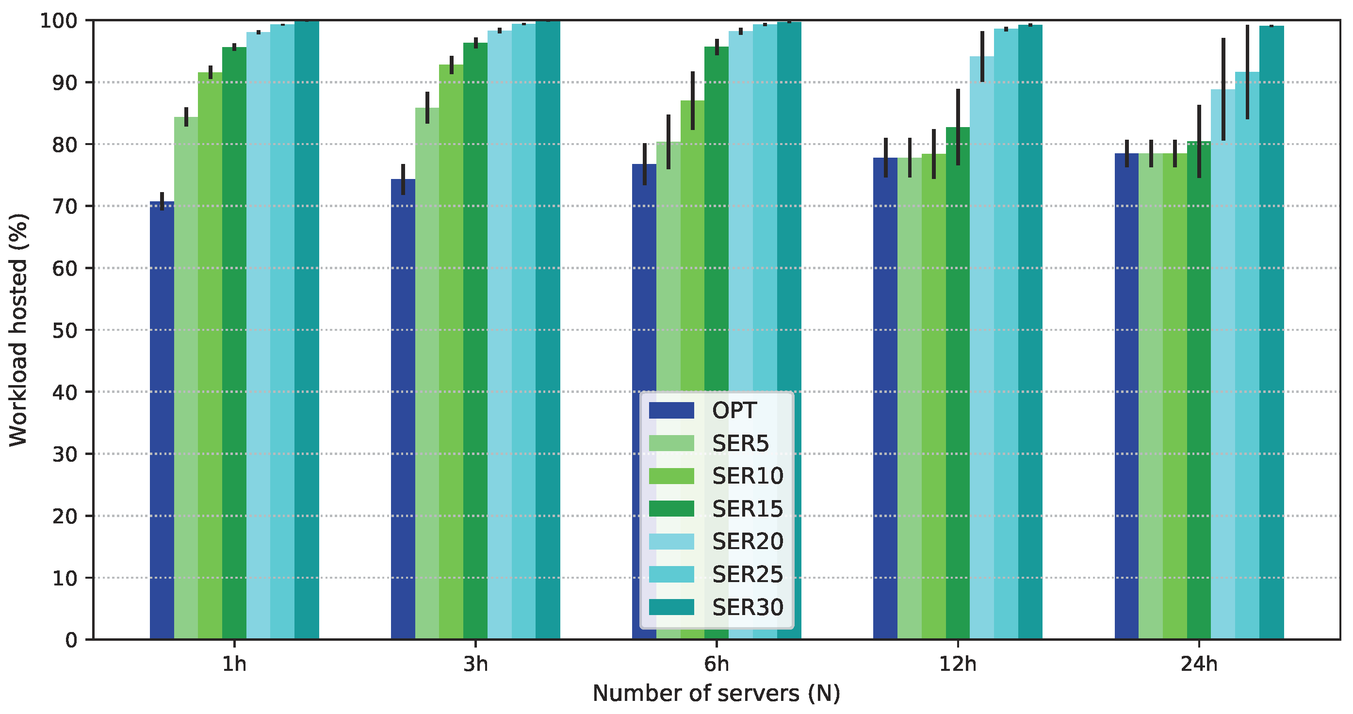
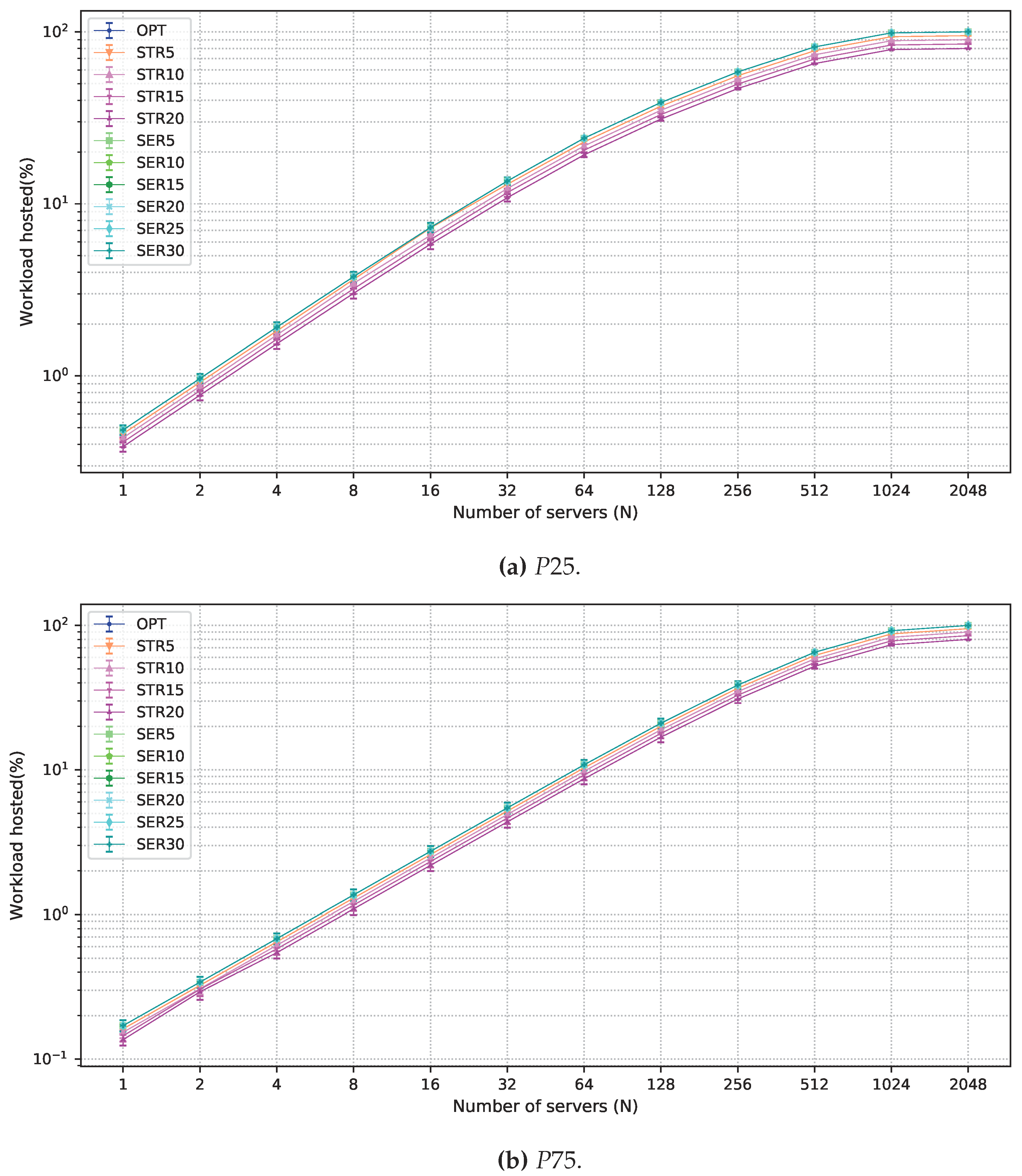
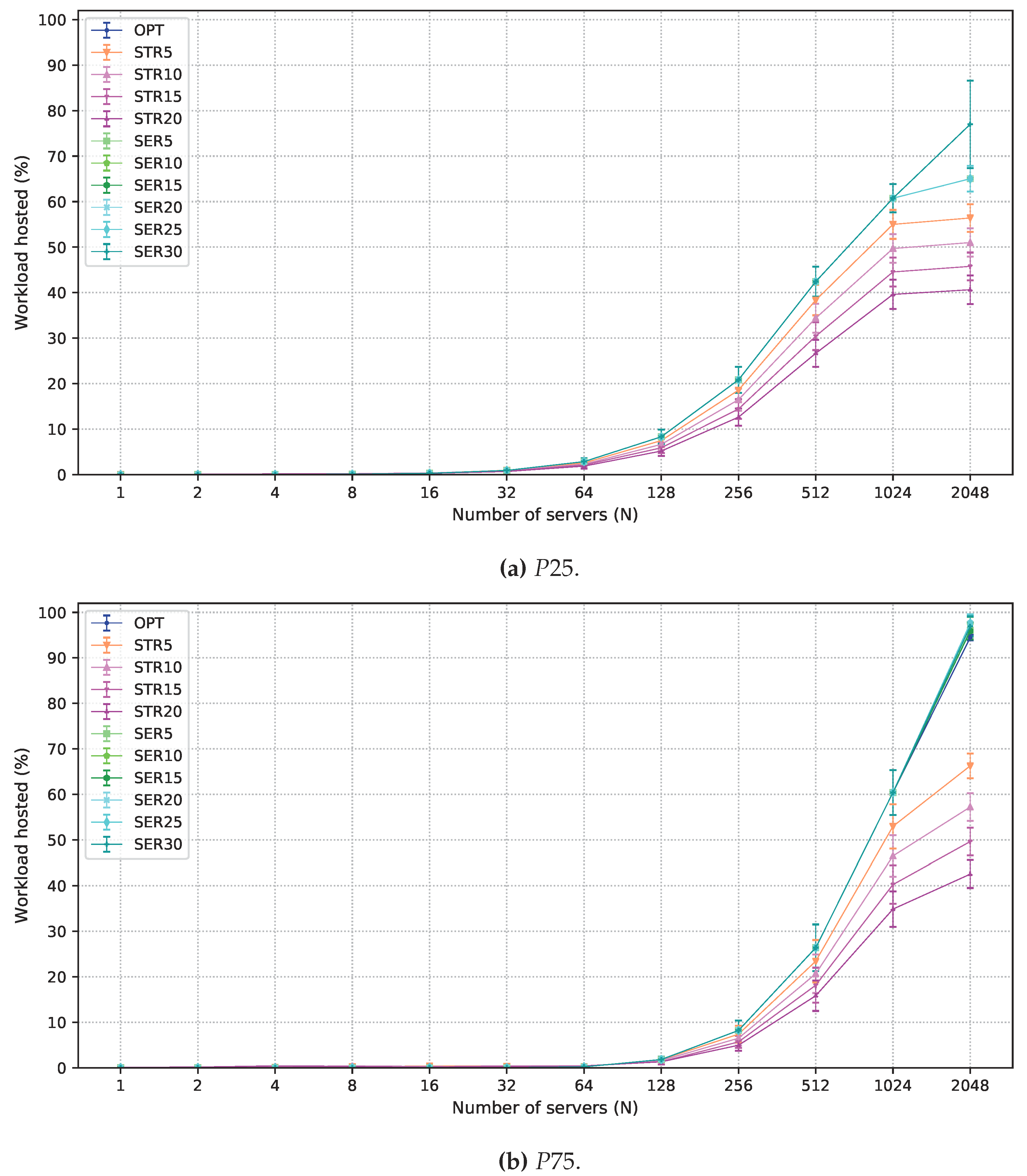
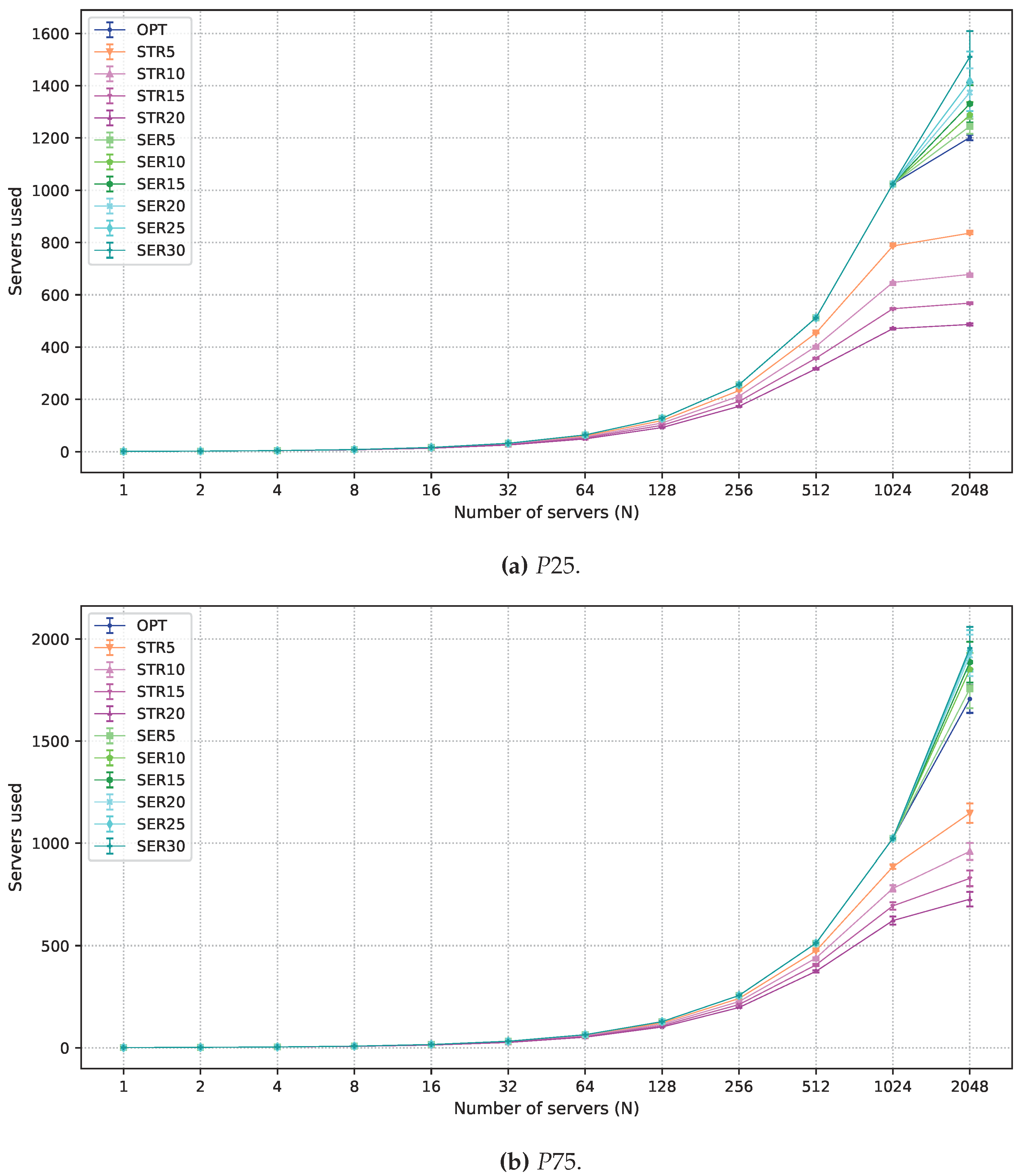
5.3. Numerical Results
6. Conclusions
Author Contributions
Funding
Conflicts of Interest
References
- Gubbi, J.; Buyya, R.; Marusic, S.; Palaniswami, M. Internet of Things (IoT): A vision, architectural elements, and future directions. Future Gener. Comput. Syst. 2013, 29, 1645–1660. [Google Scholar] [CrossRef]
- Bonomi, F.; Milito, R.; Natarajan, P.; Zhu, J. Fog Computing: A Platform for Internet of Things and Analytics. In Big Data and Internet of Things: A Roadmap for Smart Environments; Bessis, N., Dobre, C., Eds.; Springer International Publishing: Cham, Switzerland, 2014; pp. 169–186. [Google Scholar]
- da Fonseca, N.L.S.; Boutaba, R. Cloud Services, Networking, and Management; John Wiley & Sons, Ltd.: Hoboken, NJ, USA, 2015. [Google Scholar]
- OpenFog Reference Architecture. Available online: https://www.openfogconsortium.org/ra/ (accessed on 24 May 2017).
- Guevara, J.C.; Bittencourt, L.F.; da Fonseca, N.L.S. Class of service in fog computing. In Proceedings of the 2017 IEEE 9th Latin-American Conference on Communications (LATINCOM), Guatemala City, Guatemala, 8–10 November 2017; pp. 1–6. [Google Scholar] [CrossRef]
- Verbelen, T.; Simoens, P.; De Turck, F.; Dhoedt, B. Cloudlets: Bringing the Cloud to the Mobile User. In Proceedings of the Third ACM Workshop on Mobile Cloud Computing and Services, Low Wood Bay, UK, 25 June 2012; ACM: New York, NY, USA, 2012; pp. 29–36. [Google Scholar] [CrossRef]
- Marín-Tordera, E.; Masip-Bruin, X.; García-Almiñana, J.; Jukan, A.; Ren, G.J.; Zhu, J. Do we all really know what a fog node is? Current trends towards an open definition. Comput. Commun. 2017, 109, 117–130. [Google Scholar] [CrossRef]
- Vilalta, R.; Lopez, L.; Giorgetti, A.; Peng, S.; Orsini, V.; Velasco, L.; Serral-Gracia, R.; Morris, D.; De Fina, S.; Cugini, F.; et al. TelcoFog: A Unified Flexible Fog and Cloud Computing Architecture for 5G Networks. IEEE Commun. Mag. 2017, 55, 36–43. [Google Scholar] [CrossRef]
- Kim, W.; Chung, S. User-Participatory Fog Computing Architecture and Its Management Schemes for Improving Feasibility. IEEE Access 2018, 6, 20262–20278. [Google Scholar] [CrossRef]
- Souza, V.B.C.; Ramírez, W.; Masip-Bruin, X.; Marín-Tordera, E.; Ren, G.; Tashakor, G. Handling service allocation in combined Fog-cloud scenarios. In Proceedings of the 2016 IEEE International Conference on Communications (ICC), Kuala Lumpur, Malaysia, 22–27 May 2016; pp. 1–5. [Google Scholar] [CrossRef]
- da Silva, R.A.C.; da Fonseca, N.L.S. Resource Allocation Mechanism for a Fog-Cloud Infrastructure. In Proceedings of the 2018 IEEE International Conference on Communications (ICC), Kansas City, MO, USA, 20–24 May 2018; pp. 1–6. [Google Scholar] [CrossRef]
- Mahmud, R.; Ramamohanarao, K.; Buyya, R. Latency-aware Application Module Management for Fog Computing Environments. ACM Trans. Internet Technol. 2019, 19, 9. [Google Scholar] [CrossRef]
- Larumbe, F.; Sansò, B. Cloptimus: A multi-objective Cloud data center and software component location framework. In Proceedings of the 2012 IEEE 1st International Conference on Cloud Networking (CLOUDNET), Paris, France, 28–30 November 2012; pp. 23–28. [Google Scholar] [CrossRef]
- Larumbe, F.; Sansò, B. A Tabu Search Algorithm for the Location of Data Centers and Software Components in Green Cloud Computing Networks. IEEE Trans. Cloud Comput. 2013, 1, 22–35. [Google Scholar] [CrossRef]
- Covas, M.T.; Silva, C.A.; Dias, L.C. Multicriteria decision analysis for sustainable data centers location. Int. Trans. Oper. Res. 2013, 20, 269–299. [Google Scholar] [CrossRef]
- Jia, M.; Cao, J.; Liang, W. Optimal Cloudlet Placement and User to Cloudlet Allocation in Wireless Metropolitan Area Networks. IEEE Trans. Cloud Comput. 2017, 5, 725–737. [Google Scholar] [CrossRef]
- Fan, Q.; Ansari, N. Cost Aware cloudlet Placement for big data processing at the edge. In Proceedings of the 2017 IEEE International Conference on Communications (ICC), Paris, France, 21–25 May 2017; pp. 1–6. [Google Scholar] [CrossRef]
- Albareda-Sambola, M.; Fernández, E.; Hinojosa, Y.; Puerto, J. The multi-period incremental service facility location problem. Comput. Oper. Res. 2009, 36, 1356–1375. [Google Scholar] [CrossRef]
- Oliveira, E.M.R.; Viana, A.C. From routine to network deployment for data offloading in metropolitan areas. In Proceedings of the 2014 Eleventh Annual IEEE International Conference on Sensing, Communication, and Networking (SECON), Singapore, 30 June–3 July 2014; pp. 126–134. [Google Scholar] [CrossRef]
- Chen, L.; Liu, L.; Fan, X.; Li, J.; Wang, C.; Pan, G.; Jakubowicz, J.; Nguyen, T.M.T. Complementary base station clustering for cost-effective and energy-efficient cloud-RAN. In Proceedings of the 2017 IEEE SmartWorld, Ubiquitous Intelligence Computing, Advanced Trusted Computed, Scalable Computing Communications, Cloud Big Data Computing, Internet of People and Smart City Innovation (SmartWorld/SCALCOM/UIC/ATC/CBDCom/IOP/SCI), San Francisco, CA, USA, 4–8 August 2017; pp. 1–7. [Google Scholar] [CrossRef]
- Barlacchi, G.; De Nadai, M.; Larcher, R.; Casella, A.; Chitic, C.; Torrisi, G.; Antonelli, F.; Vespignani, A.; Pentland, A.; Lepri, B. A multi-source dataset of urban life in the city of Milan and the Province of Trentino. Sci. Data 2015, 2. [Google Scholar] [CrossRef] [PubMed]
- da Silva, R.A.C.; da Fonseca, N.L.S. Topology-Aware Virtual Machine Placement in Data Centers. J. Grid Comput. 2016, 14, 75–90. [Google Scholar] [CrossRef]
- Caramia, M.; Dell’Olmo, P. Multi-Objective Management in Freight Logistics; Springer: London, UK, 2008. [Google Scholar]
- OpenCellID. Available online: http://www.opencellid.org (accessed on 1 January 2019).
- Ulm, M.; Widhalm, P.; Brändle, N. Characterization of mobile phone localization errors with OpenCellID data. In Proceedings of the 2015 4th International Conference on Advanced Logistics and Transport (ICALT), Valenciennes, France, 20–22 May 2015; pp. 100–104. [Google Scholar] [CrossRef]


| Input Parameters | |
| Notation | Description |
| N | Maximum number of servers to be deployed |
| R | Capacity of a single server |
| L | Number of locations where a fog node can be created, |
| Set of all locations where a fog node can be created: | |
| T | Total number of discrete time intervals, |
| Set of all discrete time intervals: | |
| Strict workload at location at time | |
| Flexible workload at location at time | |
| Decision variables | |
| Notation | Description |
| The number of servers created at location . If , no fog node is created at location l | |
| Strict workload originating at location at time and hosted by the local fog node | |
| Flexible workload originating at location at time and hosted by the local fog node | |
| Flexible workload originating at location at time and hosted by the cloud | |
| Parameter | Values |
|---|---|
| N | 1, 2, 4, 8, 16, 32, 64, 128, 256, 512, 1024, 2048 |
| R | 1000 |
| , | |
| , each represents a ten minute interval. | |
| T varies to represent 1 h, 3 h, 6 h, 12 h, and 24 h intervals | |
| and , , | Aggregated workload of cells for each base station |
| Proportion between strict and flexible workloads | P25: 25% of strict and 75% of flexible latency workload |
| P50: 50% of strict and 50% of flexible latency workload | |
| P75: 75% of strict and 25% of flexible latency workload |
| Objective Degraded | Level of Degradation | |
|---|---|---|
| — | — | |
| Equation (1) | 5% | |
| Equation (1) | 10% | |
| Equation (1) | 15% | |
| Equation (1) | 20% | |
| Equation (2) | 5% | |
| Equation (2) | 10% | |
| Equation (2) | 15% | |
| Equation (2) | 20% | |
| Equation (2) | 25% | |
| Equation (2) | 30% |
© 2019 by the authors. Licensee MDPI, Basel, Switzerland. This article is an open access article distributed under the terms and conditions of the Creative Commons Attribution (CC BY) license (http://creativecommons.org/licenses/by/4.0/).
Share and Cite
C. da Silva, R.A.; S. da Fonseca, N.L. On the Location of Fog Nodes in Fog-Cloud Infrastructures. Sensors 2019, 19, 2445. https://doi.org/10.3390/s19112445
C. da Silva RA, S. da Fonseca NL. On the Location of Fog Nodes in Fog-Cloud Infrastructures. Sensors. 2019; 19(11):2445. https://doi.org/10.3390/s19112445
Chicago/Turabian StyleC. da Silva, Rodrigo A., and Nelson L. S. da Fonseca. 2019. "On the Location of Fog Nodes in Fog-Cloud Infrastructures" Sensors 19, no. 11: 2445. https://doi.org/10.3390/s19112445
APA StyleC. da Silva, R. A., & S. da Fonseca, N. L. (2019). On the Location of Fog Nodes in Fog-Cloud Infrastructures. Sensors, 19(11), 2445. https://doi.org/10.3390/s19112445