Abstract
This paper considers vital signs (VS) such as respiration movement detection of human subjects using an impulse ultra-wideband (UWB) through-wall radar with an improved sensing algorithm for random-noise de-noising and clutter elimination. One filter is used to improve the signal-to-noise ratio (SNR) of these VS signals. Using the wavelet packet decomposition, the standard deviation based spectral kurtosis is employed to analyze the signal characteristics to provide the distance estimate between the radar and human subject. The data size is reduced based on a defined region of interest (ROI), and this improves the system efficiency. The respiration frequency is estimated using a multiple time window selection algorithm. Experimental results are presented which illustrate the efficacy and reliability of this method. The proposed method is shown to provide better VS estimation than existing techniques in the literature.
1. Introduction
Noncontact measurement of vital signs (VS) has been the subject of significant research in recent years. It is used in applications such as health monitoring [1,2,3,4,5], heart rate variability analysis [6], monitoring chronic heart failure (CHF) patients [7], cancer radiotherapy [8], search and rescue [9], and animal health care [10,11,12,13]. Continuous wave (CW) radar has been used extensively for VS detection [14,15,16,17,18,19,20,21]. Many detection techniques have been proposed in the literature [22,23,24,25,26,27,28,29,30,31,32,33,34,35,36,37,38,39,40,41]. Ultra-wideband (UWB) impulse radar is one of the most effective methods for VS detection due to the high resolution and penetrability and low-power radiation [11,12,13,14,15].
A variable time window algorithm was used to estimate the human heart rate in [4]. Human cardiac and respiratory movements have been analysed using the fast Fourier transform (FFT) and Hilbert–Huang transform (HHT) [22,23]. To avoid the codomain restriction in arctangent demodulation (AD), an extended differentiate and cross-multiply (DACM) method was proposed in [24]. In [25], respiration-like clutter was suppressed using an adaptive cancellation method. A phase-based method is proposed to detect the heart rate based on the UWB impulse Doppler radar [26]. A short-time Fourier transform (STFT) was used for VS detection in [27]. However, these methods cannot accurately estimate the frequencies of VS signals due to the presence of harmonics. Further, STFT performance is sensitive to the window length. Ensemble empirical mode decomposition (EEMD) and a frequency window were used to remove clutter and harmonics in [28], but this increases the receiver complexity. In [28], singular value decomposition (SVD) was employed to detect the period of human respiration signals in very low signal to noise and clutter ratio (SNCR) environments. An adaptive Kalman filter was developed to extract respiration signals from UWB radar data in [29]. However, incorrect results were obtained when no subject was present. A constant false alarm rate (CFAR) technique was used in [32] to remove clutter and improve the SNR of VS signals. Static clutter was removed using linear trend subtraction (LTS) in [34]. In [36], a higher order cumulant (HOC) method was used to suppress noise based on the fact that the noise can be approximated as Gaussian. In [37], an EEMD method was presented to analyse human heart rate variations. An extended complex signal demodulation (CSD) technique was considered in [38] to eliminate the wrapped problem with the DACM algorithm. A state space (SS) method was proposed in [40] for VS detection over short distances. The usefulness of these algorithms is limited by the complexity of real VS signal environments. In particular, they are not effective for clutter removal, respiration signal extraction, and respiration and heart rate estimation in long distance and through-wall conditions. As a result, improved techniques are required for VS signal detection.
In this paper, a new method is presented to accurately estimate VS parameters even in low SNR conditions such as long range and through-wall. The time of arrival (TOA) is determined using the wavelet transform (WT) of the kurtosis and standard deviation (SD) of the received UWB signals. Further, a method to estimate the respiration frequency is presented. The performance of this method is compared with that of several well-known algorithms using data obtained with the UWB radar designed by the Key Laboratory of Electromagnetic Radiation and Sensing Technology, Institute of Electronics, Chinese Academy of Sciences. The contributions of the paper can be summarized as:
- The signal to noise and clutter ratio (SNCR) of the received UWB pulses is improved using an improved filter.
- Based on the distance estimate, the region of interest (ROI) containing VS signals is defined to reduce the data size and improve the system efficiency.
- To obtain the respiration frequency more accurately, the time window selection algorithm is proposed to remove the random noise.
2. Vital Sign Model
A model similar to that in [36] for UWB impulse radar signals is employed here. Slow time denotes the received pulses while fast time represents the range. Figure 1 illustrates the received pulses which have been modulated by the periodic human respiration movements [27].

Figure 1.
An illustration of the received radar pulses.
The distance can be expressed as
where is the distance between the center of the human thorax and the radar, t is the slow time, is the respiration amplitude, and is the respiration frequency. The received UWB impulse radar signal is
where denotes convolution, is the transmitted UWB pulse, τ is the fast time, is the pulse period, n is the slow time index with samples, is the time delay from UWB radar to the human subject, r denotes the response from human respiratory movements, is the response from the human subject, P is the number of the static objects, is the time delay from UWB radar to other objects, is the response from all other objects, is the linear trend, is additive white Gaussian noise (AWGN), is nonstatic clutter, and is unknown clutter. The time delay can be expressed as
where and , v is the light speed. The fast time period is with sampling interval . The received signal can be expressed as a matrix with elements
where m is the fast time index and M is the corresponding number of samples, is the received pulses from human subject in digital form, is the received pulses from static object in digital form, is the linear trend in digital form, is AWGN in digital form, is non-static clutter in digital form and is unknown clutter in digital form.
In a static environment, the ideal signal after clutter removal is
Taking the Fourier transform (FT) gives
and the two dimensional (2-D) FT gives
where
is the FT of a UWB pulse, f is the spectrums of the slow time, and υ is the spectrums of the fast time.
Using Bessel functions, Formula (12) can be expressed as
We have
where , and , so then Formula (7) is given by
where
When , the maximum of Formula (13) is obtained as
The respiratory signal with is given by
However, linear trend, non-static clutter, and other clutter exist in the received signals. This along with AWGN makes detection difficult, as can be seen by comparing Figure 2a,b which show a respiration signal without and with AWGN [30], respectively.

Figure 2.
The time-range matrix with (a) only the respiration signal, and (b) the signal with additive white Gaussian noise (AWGN) at an SNR of −10 dB.
3. VS Detection Algorithm
A flowchart of the proposed detection method is given in Figure 3 and the steps are described below. Five healthy volunteers from the Key Laboratory of Electromagnetic Radiation and Sensing Technology, Institute of Electronics, participated in this research. All participants consented to participate and were informed of the associated risks. The experiments were approved by both Ocean University of China and the Chinese Academy of Sciences and were performed in accordance with the relevant international guidelines and regulations.

Figure 3.
Flowchart of the proposed detection method.
3.1. Clutter Suppression
VS signals are typically corrupted by significant static clutter which can be estimated as
and the signal after cancellation is
The LTS algorithm can be used to remove the linear trend term expressed as [27,30]
where , , , and T denotes the matrix transpose.
3.2. SNR Improvement
The received signal depends on the dielectric constant, humidity, and polarization of the electromagnetic wave, and estimating these values can be difficult [36]. Therefore, a bandpass filter is used rather than a matched filter. In this paper, two fifth-order Butterworth filters are employed, a low-pass filter with normalized cutoff frequency 0.1037 and a high-pass filter with normalized cut off frequency 0.0222. The filter output is
where and are the coefficient vectors. A smoothing filter which averages seven values in slow time is used to improve SNR which gives
where and is the largest integer less than .
3.3. TOA Estimation
Gaussian noise is a major factor affecting VS signals. The spectral kurtosis can be used to extract non-Gaussian signals and their position in frequency [42,43] and has been employed in many applications [44,45,46,47,48]. An improved TOA estimation algorithm is presented here, which is based on the standard deviation (SD) and kurtosis.
The kurtosis for each fast time index m in is given by [44]
where denotes expectation. The kurtosis is three for a Gaussian distribution [45] and the excess kurtosis is given by
The excess kurtosis is considered in this paper, and this is given in Figure 4a for the data acquired with a volunteer located at a distance of 9 m from the radar outdoors. This shows that the difference in excess kurtosis between when a target is present and not present is small. Thus the SD is combined with the excess kurtosis.

Figure 4.
The (a) excess kurtosis, and (b) the kurtosis to SD (KSD) with a human subject, the (c) KSD without a human subject, (d) KSD in the target area, and (e) the spectrum of (d).
The SD is given by [44]
And the kurtosis to SD (KSD) is defined as . Figure 4b shows the KSD for the radar data described above. This indicates that there is a significant difference in the KSD between when a subject is present and not present. Figure 4d shows that the KSD in the target area is approximately periodic. Figure 4d gives the FTT of the KSD in Figure 4d, which confirms the KSD periodicity. The KSD when a subject is not present is shown in Figure 4c.
The STFT [49,50,51] and wavelet transform (WT) [52,53,54] have been widely used to analyze VS signals. However, the STFT performance depends on the length which can be difficult to determine. As a consequence, the WT is considered here as it also provides the advantage of scalability in the frequency domain [55]. For a given time domain signal , the continuous WT is
where is the wavelet with scaling parameter and translation parameter , and ¯ denotes complex conjugate.
The Morlet wavelet is considered here as it is widely used because of its simple implementation and is given by
The discrete WT is employed in this paper, which is
The resulting time-frequency matrix when a target is present is shown in Figure 5a and when a target is not present in Figure 5b. The VS signal is indicated in the red region. The range between the radar receiver and target can be estimated as
where is TOA estimate corresponding to the maximum value in the matrix.
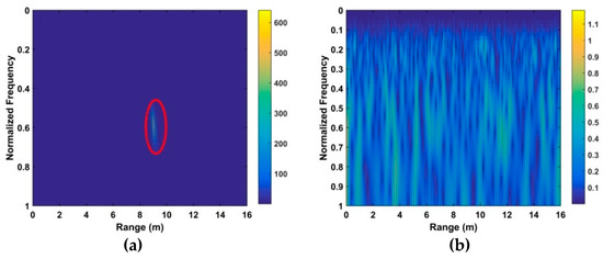
Figure 5.
The time-frequency matrix using the wavelet transform (WT) decomposition (a) with a human subject at 9 m and (b) without a subject.
3.4. Frequency Estimation
3.4.1. Data Reduction
The index of the TOA estimate in can be expressed as
The human respiration frequency is usually between 0.2 and 0.4 Hz with amplitude 0.5 to 1.5 cm [56]. Thus, , which has a range of approximately 8 cm is considered as the region of interest (ROI) containing the respiration signal. ROI constants for all the human subjects, and it is independent of the height, weight, size of the person. Figure 6a shows a slow time signal in the ROI, while a slow time signal not in the ROI is given in Figure 6b. To further illustrate the differences, Figure 6c shows 10 randomly selected slow time signals in the ROI, Figure 6d shows 10 randomly selected slow time signals not in the ROI, and Figure 6e shows all the slow time signals in the ROI. These show that the transmitted radar signals have been modulated by the human respiration signal. Thus, only signals in the ROI are used to estimate the respiration frequency. In the radar system, 4096 × N samples are to reduce the amount data to be analyzed and improve performance.

Figure 6.
Signals in the time-frequency matrix (a) one in the region of interest (ROI), (b) one not in the ROI, (c) ten in the ROI, (d) ten not in the ROI and (e) all in the ROI.
3.4.2. Noise Removal
To estimate the respiration frequency more accurately, the wavelet packet decomposition of each slow time signal in the ROI is used [57,58]. For each slow time signal in Figure 6a where , we have
where
are the scaling coefficients and
are the wavelets.
The corresponding Welch power spectrums of the individual wavelets are given in Figure 7 [59]. The x-axis is normalized frequency which is given by
where denotes the slow time sampling frequency. This figure shows that d6 is concentrated in the 0.1 to 0.5 Hz frequency range, while the other wavelets are concentrated in higher (>1 Hz) or lower (<0.1 Hz) frequencies. As a result, to reduce noise the VS signals are extracted using d6.

Figure 7.
The Welch power spectrum of (a) d1, (b) d2, (c) d3, (d) d4, (e) d5, (f) d6, (g) d7, and (h) d8.
3.4.3. Spectral Analysis
As mentioned above, the respiration period is between 2.5 and 5 s. As a result, it is challenging to estimate the respiration frequency accurately using a time window of less than 5 s. Further, the estimation accuracy is affected by inhomogeneous respiration, so the time window should be at least 3 to 6 periods [4]. An FFT is performed on d6 and the maximum value is the respiration frequency estimate.
For a time window , the resolution is
Accurate estimation requires that
so
where is an integer chosen to satisfy Formula (35).
Figure 8a shows the time windows used which are given by
where is the length of the ith window and ς denotes the increase in length. Increasing the window length improves the frequency resolution which is given by
where is the sampling frequency, and ς satisfies [4]

Figure 8.
The time windows with (a) increasing length, and (b) fixed length.
This increase in window length results in an increase in the complexity of the radar system as multiple FFTs must be computed. Further, this approach cannot reduce the harmonics of the respiration signal [4] due to the different frequency spectrum lengths.
To improve the frequency resolution and reduce the harmonics while keeping the complexity reasonable, another multiple time window technique is employed which is shown in Figure 8b. In this case, the time windows have the same length so the frequency resolution is
where is the length of the ith window, and q is the number of windows.
The radar system can only process data of length . Therefore, the window length is chosen to be wi = 512 samples with an overlap of G = 256 in Figure 8b. Each radar measurement provides 1024 samples, so q = 3 sets of data are acquired for, . Thus, the system parameters are N = 512, Hz, and .
A frequency window of 0.1 to 0.8 Hz was previously used to reduce the clutter and improve SNR. However, a window is not necessary with the proposed approach due to the defined ROI. As a result, only an FFT is performed on each signal
Cumulants are employed to remove harmonics and clutter
The frequency is then estimated as
where corresponds to the index of the maximum value in Formula (37).
4. Data Acquisition
4.1. UWB Impulse Radar
Figure 9a shows the UWB impulse radar used for data acquisition. It contains one transmitter and one receiver and is controlled by a wireless personal digital assistant. Table 1 gives the system parameters. The UWB pulses are transmitted with a 400 MHz center frequency and a 600 kHz pulse repetition frequency. The data are obtained for 124 ns time windows. M = 4096 samples are obtained in fast time and N = 512 pulses in slow time which requires 17.6 s. A combination of the equivalent-time [60] and real-time [61] sampling methods is employed which provides better performance than with only one method. Figure 9b shows the received signal matrix R obtained with one male volunteer outdoors at a distance of 9 m from the radar. The VS signal is not noticeable because of the large path loss due to the long-range and through-wall conditions. This indicates that VS signal detection in real environments is challenging.

Figure 9.
(a) The UWB radar and (b) the data for the first experiment with a human subject at a distance of 9 m from the radar.

Table 1.
The UMB Impulse Radar Parameters.
4.2. Experimental Setup
The experiments were conducted at the Institute of Electronics, Chinese Academy of Sciences and the China National Fire Equipment Quality Supervision Centre. The experimental setups are illustrated in Figure 10a,b. The human subjects faced the radar breathing normally and kept still.

Figure 10.
The experimental setup for (a) subjects in front of the radar, (b) subjects at an angle to the radar, (c) through-wall detection outdoors, (d) through-wall detection indoors and (e) the actuator.
The first experiment was conducted outdoors at the Institute of Electronics as shown in Figure 10c at distances of 6 m, 9 m, 11 m and 14 m with two female (158 cm, 48 kg and 163 cm, 54 kg) and two male (178 cm, 84 kg and 182 cm, 76 kg) subjects. This environment includes vegetation with moves in the wind. The wall is 2.7 m high and more than 10 m wide, and is composed of three different materials including 30 cm of brick, 35 cm of concrete, and 35 cm of pine. The radar is located at a height of 1.5 m. The second experiment was conducted indoors at the China National Fire Equipment Quality Supervision Center as shown in Figure 10d at distances of 7 m, 10 m, 12 m and 15 m with one male subject (172 cm, 74 kg). The wall is 2.5 m in height and 3 m in width. The radar is located at a height of 1.3 m.
The third experiment was conducted indoors at the China National Fire Equipment Quality Supervision Center as shown in Figure 10e at distances of 7 m, 10 m and 12 m using an actuator of size 0.25 × 0.3 m2 to imitate human respiration. The actuator was on a desk 1.3 m above ground and moved at an amplitude of 3 mm and a frequency of 0.3333 Hz. In the fourth experiment, the actuator was on a desk 70 cm above ground at a distance of 6 m outdoors at the Institute of Electronics. In the fifth experiment, the actuator was on a desk 1.3-m above ground at azimuth angles of 30° and 60°with respect to the radar antenna indoors at a distance of 6 m as illustrated in Figure 10b.
5. Experimental Results
In this section, the performance of the proposed algorithm is compared with the FFT, constant false alarm rate (CFAR) [32], advanced [35], and multiple higher order cumulant (MHOC) [36] methods which are well-known in the literature. The clutter removal and SNR improvement are evaluated using data from the first experiment with a female subject (158 cm, 48 kg) located 9 m from the radar. Figure 11 shows the received signal for 18 s. The result after LTS is given in Figure 11a. This indicates that although the amplitude of the received signal is decreased, the VS signal is more pronounced. Figure 11b gives the result after filtering in fast time (range), and Figure 11c after filtering in slow time. This shows that the VS signal is more visible after filtering.

Figure 11.
The results for the first experiment after (a) linear trend suppression (LTS), (b) range (fast time) filtering and (c) slow time filtering.
5.1. Vital Sign Estimation Outdoors
The TOA and frequency estimation performance are now examined using the data from experiment one with four subjects at different distances. The KSD, TOA, and frequency estimation are first obtained with one female subject (158 cm, 48 kg). Figure 12 presents the KSD for the four distances which shows that the KSD is larger in the ROI. The range results after WT decomposition of the KSD are shown in Figure 13. The range errors are 0.12 m at 6 m, 0.17 m at 9 m, 0.11 m at 11 m and 0.14 m at 14 m. The slow time signals in the ROI at the four distances are given in Figure 14. All indicate modulation by human respiration. Figure 15 presents the corresponding frequency estimation which gives values of 0.26 Hz at 6 m, 0.31 Hz at 9 m, 0.31 Hz at 11 m and 0.26 Hz at 14 m. Further, it indicates that the harmonics have been effectively suppressed.

Figure 12.
The KSD for the first experiment at distances of (a) 6 m, (b) 9 m, (c) 11 m and (d) 14 m from the radar.

Figure 13.
Range estimation for the first experiment at distances of (a) 6 m, (b) 9 m, (c) 11 m and (d) 14 m from the radar.


Figure 14.
The signal in the ROI for the first experiment at distances of (a) 6 m, (b) 9 m, (c) 11 m and (d) 14 m from the radar.

Figure 15.
Frequency estimation for the first experiment at distances of (a) 6 m, (b) 9 m, (c) 11 m and (d) 14 m from the radar.
The SNR of the VS signal can be expressed as [37]
where is the zero frequency index and is the index of . Figure 16 gives the results for the CFAR method with subject III, and the corresponding advanced method (AM) results are shown in Figure 17. The red squares denote the estimates while the black ellipses denote the true values. These figures show that these methods cannot provide accurate range estimates, while the previous results indicate that the proposed method performs well even at a distance of 14 m. The frequency estimates and corresponding SNRs for the four subjects with the proposed algorithm are given in Table 2. Table 3 presents the results with subject I for four different algorithms. These tables show that the proposed method provides more accurate range and frequency estimates, and high SNRs.

Figure 16.
Results using the CFAR method for subject III in the first experiment at distances of (a) 6 m, (b) 9 m and (c) 11 m from the radar.

Figure 17.
Results using AM for subject III in the first experiment at distances of (a) 6 m, (b) 9 m and (c) 11 m from the radar.
Table 2.
VS Estimates for Four Subjects at Different Distances.
Table 3.
Performance for Subject I with Four Methods.
5.2. VS Estimation Indoors
The data from the second experiment obtained indoors at the China National Fire Equipment Quality Supervision Center with a male subject (172 cm, 74 kg) is now considered. Figure 18 shows the KSD for distances of 7 m, 10 m, 12 m and 15 m. The range estimates after WT decomposition of the KSD are given in Figure 19. The corresponding errors are 0.04 m at 7 m, 0.05 m at 10 m, 0.08 m at 12 m and 0.07 m at 15 m. These results indicate that the range is estimated more accurately indoors, largely due to the fact that the wind causes movement in the environment.


Figure 18.
The KSD for the second experiment at distances of (a) 7 m, (b) 10 m, (c) 12 m and (d) 15 m from the radar.

Figure 19.
Range estimation for the second experiment at distances of (a) 7 m, (b) 10 m, (c) 12 m and (d) 15 m from the radar.
Figure 20 shows the frequency estimation results and the estimates are 0.37 Hz at 7 m, 0.31 Hz at 10 m, 0.31 Hz at 12 m and 0.37 Hz at 15 m. The frequency estimates, SNRs and range errors for three methods are given in Table 4. The FFT method has the worst performance and cannot provide accurate frequency and range estimates. Adding a frequency window after the FFT can improve the SNR [62], but the range and frequency estimates are still poor, especially at long distances. Conversely, the proposed method has excellent performance at all distances.

Figure 20.
Frequency estimation for the second experiment at distances of (a) 7 m, (b) 10 m, (c) 12 m and (d) 15 m from the radar.
Table 4.
VS Estimates for Three Distances.
5.3. Actuator Signal Estimation
The KSD for the data from experiment three is shown in Figure 21. The corresponding range estimates obtained using WT decomposition are given in Figure 22, and the signals in the ROI are shown in Figure 23. Comparing Figure 14 and Figure 23, the modulation is more pronounced with the actuator than with human respiration. Figure 24 shows the frequency estimation and the estimates are 0.34 Hz at 7 m, 0.32 Hz at 10 m and 0.33 Hz at 12 m. The corresponding deviations are 0.66%, 0.33%, and 0.24%, respectively. The results for four algorithms are given in Table 5. Again the proposed method is the best. The detection results using the data from experiment four are shown in Figure 25. This shows that the proposed algorithm provides better range and frequency estimates compared to the other methods.

Figure 21.
The KSD for the third experiment at distances of (a) 7 m, (b) 10 m and (c) 12 m from the radar.

Figure 22.
Third experiment range estimation at distances of (a) 7 m, (b) 10 m and (c) 12 m from the radar.

Figure 23.
The signal in the ROI for the third experiment at distances of (a) 7 m, (b) 10 m and (c) 12 m from the radar.

Figure 24.
Third experiment frequency estimation at distances of (a) 7 m, (b) 10 m and (c) 12 m from the radar.
Table 5.
Results with Four Methods at Different Distances.

Figure 25.
Results for the fourth experiment with the actuator outdoors (a) KSD, (b) range estimation and (c) the signal in the ROI.
5.4. Estimation at Different Azimuth Angles
The influence of the azimuth angle between the subject and radar on the detection performance is now examined. The beam angle of the antenna in the radar system is 60°. In previous sections, the subject and actuator were directly in front of the radar so the azimuth angle was 0°. In this section, results are obtained for the data from experiment five with the actuator at a distance of 6 m and angles of 30 and 60. Figure 26 presents the KSD and range estimates, and the signals in the ROI are shown in Figure 27. Table 6 compares the results for the proposed algorithm with three other methods. This indicates that the proposed algorithm provides superior performance, particularly at a 60°angle. AM has a better frequency estimate at 30°but the range error is very high.

Figure 26.
The results for the fifth experiment (a) KSD at 30°, (b) range at 30°, (c) KSD at 60° and (d) range at 60°.

Figure 27.
The signals in the ROI for the fifth experiment at angles of (a) 30° and (b) 60°.
Table 6.
Results for Different Azimuth Angles.
6. Conclusions
In this paper, a new method for human respiration movement detection was presented based on an UWB impulse radar. The time of arrival (TOA) of the received UWB signals was estimated using a wavelet transform (WT), and the human respiration frequency was estimated using a time window technique. The performance of the proposed method was compared with several well-known algorithms under different indoor and outdoor conditions. The results obtained indicate that this technique can effectively suppress clutter and provides superior detection performance.
Author Contributions
conceptualization, M.S.F. and X.L.; methodology, T.L, X.L.; software, X.L.; validation, X.L., M.S.F.; formal analysis, X.L.; investigation, M.S.F. and X.L.; resources, X.L.; writing—original draft preparation, M.S.F. and X.L.; writing—review and editing, T.A.G.; visualization, T.L.; funding acquisition, H.Z.
Funding
This research was funded by the National Natural Science Foundation of China (61701462, 61501424 and 41527901), National High Technology Research and Development Program of China (2012AA061403), National Science & Technology Pillar Program during the Twelfth Five-year Plan Period (2014BAK12B00), Ao Shan Science and Technology Innovation Project of Qingdao National Laboratory for Marine Science and Technology (2017ASKJ01), Qingdao Science and Technology Plan (17-1-1-7-jch), and the Fundamental Research Funds for the Central Universities (201713018).
Acknowledgments
The authors would like to thank the anonymous reviewers for their valuable comments and suggestions to improve the quality of the article.
Conflicts of Interest
The authors declare no conflict of interest.
References
- Kranjec, K.; Beguš, S.; Drnovšek, J.; Gersak, G. Novel methods for noncontact heart rate measurement: A feasibility study. IEEE Trans. Instrum. Meas. 2014, 63, 838–847. [Google Scholar] [CrossRef]
- Zhao, H.; Hong, H.; Sun, L.; Li, Y.; Li, C.; Zhu, X. Noncontact physiological dynamics detection using low-power digital-IF Doppler radar. IEEE Trans. Instrum. Meas. 2017, 66, 1780–1788. [Google Scholar] [CrossRef]
- Kazemi, S.; Ghorbani, A.; Amindavar, H.; Morgan, D.R. Vital-sign extraction using bootstrap-based generalized warblet transform in heart and respiration monitoring radar system. IEEE Trans. Instrum. Meas. 2016, 65, 255–263. [Google Scholar] [CrossRef]
- Khan, F.; Sung, H.C. A detailed algorithm for vital sign monitoring of a stationary/non-stationary human through ir-uwb radar. Sensors 2017, 17, 290. [Google Scholar] [CrossRef]
- Leem, S.K.; Faheem, K.; Sung, H.C. Vital Sign Monitoring and Mobile Phone Usage Detection Using IR-UWB Radar for Intended Use in Car Crash Prevention. Sensors 2017, 17, 1240. [Google Scholar] [CrossRef] [PubMed]
- Ahmad, S.; Bolic, M.; Dajani, H.; Groza, V.; Batkin, I.; Rajan, S. Measurement of heart rate variability using an oscillometric blood pressure monitor. IEEE Trans. Instrum. Meas. 2010, 59, 2575–2590. [Google Scholar] [CrossRef]
- Fanucci, L.; Saponara, S.; Bacchillone, T.; Donati, M.; Barba, T.; Sanchez-Tato, I.; Carmona, C. Sensing devices and sensor signal processing for remote monitoring of vital signs in CHF patients. IEEE Trans. Instrum. Meas. 2013, 62, 553–569. [Google Scholar] [CrossRef]
- Gu, C.; Li, R.; Zhang, H.; Fung, A.Y.C.; Torres, C.; Jiang, S.B.; Li, C. Accurate respiration measurement using DC-coupled continuous-wave radar sensor for motion-adaptive cancer radiotherapy. IEEE Trans. Biomed. Eng. 2012, 59, 3117–3123. [Google Scholar]
- Chen, K.M.; Huang, Y.; Zhang, J.; Norman, A. Microwave life-detection systems for searching human subjects under earthquake rubble or behind barrier. IEEE Trans. Biomed. Eng. 2000, 47, 105–114. [Google Scholar] [CrossRef] [PubMed]
- Hafner, N.; Drazen, J.C.; Lubecke, V.W. Fish heart rate monitoring by body-contact Doppler radar. IEEE Sens. J. 2012, 13, 408–414. [Google Scholar] [CrossRef]
- Li, J.; Liu, L.; Zeng, Z.; Liu, F. Advanced signal processing for vital sign extraction with applications in UWB radar detection of trapped victims in complex environments. IEEE J. Sel. Top. Appl. Earth Obs. Remote Sens. 2014, 7, 783–791. [Google Scholar]
- Wang, Z.; Zhang, H.; Lu, T.; Gulliver, A. Cooperative RSS-based Localization in Wireless Sensor Networks Using Relative Error Estimation and Semidefinite Programming. IEEE T. Veh. Technol. 2018. [Google Scholar] [CrossRef]
- Hu, W.; Zhao, Z.; Wang, Y.; Zhang, H.; Lin, F. Noncontact accurate measurement of cardiopulmonary activity using a compact quadrature Doppler radar sensor. IEEE Trans. Biomed. Eng. 2014, 61, 725–735. [Google Scholar]
- Astola, J.T.; Egiazarian, K.O.; Khlopov, G.I.; Khomenko, S.I.; Kurbatov, I.V.; Morozov, V.Y.; Totsky, A.V. Application of bispectrum estimation for time-frequency analysis of ground surveillance Doppler radar echo signals. IEEE Trans. Instrum. Meas. 2008, 57, 1949–1957. [Google Scholar] [CrossRef]
- Lee, J.S.; Nguyen, C.; Scullion, T. A novel, compact, low-cost, impulse ground-penetrating radar for nondestructive evaluation of pavements. IEEE Trans. Instrum. Meas. 2004, 53, 1502–1509. [Google Scholar] [CrossRef]
- JalaliBidgoli, F.; Moghadami, S.; Ardalan, S. A compact portable microwave life-detection device for finding survivors. IEEE Embed. Syst. Lett. 2016, 8, 10–13. [Google Scholar] [CrossRef]
- Gennarelli, G.; Ludeno, G.; Soldovieri, F. Real-time through-wall situation awareness using a microwave Doppler radar sensor. Remote Sens. 2016, 8, 621. [Google Scholar] [CrossRef]
- Guan, S.; Rice, J.A.; Li, C.; Gu, C. Automated DC offset calibration strategy for structural health monitoring based on portable CW radar sensor. IEEE Trans. Instrum. Meas. 2014, 63, 3111–3118. [Google Scholar] [CrossRef]
- Kuutti, J.; Paukkunen, M.; Aalto, M.; Eskelinen, P.; Sepponen, R.E. Evaluation of a Doppler radar sensor system for vital signs detection and activity monitoring in a radio-frequency shielded room. Measurement 2015, 68, 135–142. [Google Scholar] [CrossRef]
- Droitcour, A.D.; Boric-Lubecke, O.; Lubecke, V.M.; Lin, J. Range correlation and I/Q performance benefits in single-chip silicon Doppler radars for noncontact cardiopulmonary monitoring. IEEE Trans. Microw. Theory Tech. 2004, 52, 838–848. [Google Scholar] [CrossRef]
- Wang, F.K.; Horng, T.S.; Peng, K.C.; Jau, J.K.; Li, J.Y.; Chen, C.C. Single-antenna Doppler radars using self and mutual injection locking for vital sign detection with random body movement cancellation. IEEE Trans. Microw. Theory Tech. 2011, 59, 3577–3587. [Google Scholar] [CrossRef]
- Liu, L.; Liu, Z.; Barrowes, B. Through-wall bio-radiolocation with UWB impulse radar-Observation, simulation and signal extraction. IEEE J. Sel. Top. Appl. Earth Obs. Remote Sens. 2011, 4, 791–798. [Google Scholar] [CrossRef]
- Liu, L.; Liu, Z.; Xie, H.; Barrowes, B.; Bagtzoglou, A.C. Numerical simulation of UWB impulse radar vital sign detection at an earthquake disaster site. Ad Hoc Netw. 2014, 13, 34–41. [Google Scholar] [CrossRef]
- Wang, J.; Wang, X.; Chen, L.; Huangfu, J.; Li, C.; Ran, L. Noncontact distance and amplitude-independent vibration measurement based on an extended DACM algorithm. IEEE Trans. Instrum. Meas. 2014, 63, 145–153. [Google Scholar] [CrossRef]
- Li, Z.; Li, W.; Lv, H.; Zhang, Y.; Jing, X.; Wang, J. A novel method for respiration-like clutter cancellation in life detection by dual-frequency IR-UWB radar. IEEE Trans. Microw. Theory Tech. 2013, 61, 2086–2092. [Google Scholar] [CrossRef]
- Ren, L.; Wang, H.; Naishadham, K.; Kilic, O.; Fathy, A.E. Phase-based methods for heart rate detection using UWB impulse Doppler radar. IEEE Trans. Microw. Theory Tech. 2016, 64, 3319–3331. [Google Scholar] [CrossRef]
- Liang, X.; Zhang, H.; Ye, S.; Fang, G.; Gulliver, T.A. Improved denoising method for through-wall vital sign detection using UWB impulse radar. Digit. Signal. Process. 2018, 74, 72–93. [Google Scholar] [CrossRef]
- Nezirovíc, A.; Yarovoy, A.G.; Ligthart, L.P. Signal processing for improved detection of trapped victims using UWB radar. IEEE Trans. Geosci. Remote Sens. 2010, 48, 2005–2014. [Google Scholar] [CrossRef]
- Lv, H.; Qi, F.; Zhang, Y.; Jiao, T.; Liang, F.; Li, Z.; Wang, J. Improved detection of human respiration using data fusion based on a multistatic UWB radar. Remote Sens. 2016, 8, 773. [Google Scholar] [CrossRef]
- Liang, X.; Zhang, H.; Gulliver, T.A.; Fang, G.; Ye, S. An improved algorithm for through-wall target detection using ultra-wideband impulse radar. IEEE Access 2017, 5, 22101–22118. [Google Scholar] [CrossRef]
- Liang, X.; Wang, Y.; Wu, S.; Gulliver, T.A. Experimental Study of Wireless Monitoring of Human Respiratory Movements Using UWB Impulse Radar Systems. Sensors 2018, 18, 3065. [Google Scholar] [CrossRef] [PubMed]
- Xu, Y.; Wu, S.; Chen, C.; Chen, J.; Fang, G. A novel method for automatic detection of trapped victims by ultrawideband radar. IEEE Trans. Geosci. Remote Sens. 2012, 50, 3132–3142. [Google Scholar] [CrossRef]
- Xie, Y.; Fang, G. Equi-amplitude tracing algorithm based on base-band pulse signal in vital sign detecting. Electron. Inf. Technol. 2009, 31, 1132–1135. [Google Scholar]
- Hu, W.; Zhao, Z.; Wang, Y.; Zhang, H.; Lin, F. Noncontact accurate measurement of cardiopulmonary activity using a compact quadrature Doppler radar sensor. IEEE Trans. Biomed. Eng. 2014, 61, 725–735. [Google Scholar] [CrossRef] [PubMed]
- Wu, S.; Tan, K.; Xia, Z.; Chen, J. Improved human respiration detection method via ultra-wideband radar in through-wall or other similar conditions. IET Radar Sonar Navig. 2016, 10, 468–476. [Google Scholar] [CrossRef]
- Xu, Y.; Wu, S.; Chen, C.; Chen, J.; Fang, G. Vital sign detection method based on multiple higher order cumulant for ultra-wideband radar. IEEE Trans. Geosci. Remote Sens. 2012, 50, 1254–1265. [Google Scholar] [CrossRef]
- Hu, X.; Jin, T. Short-range vital signs sensing based on EEMD and CWT using IR-UWB radar. Sensors 2016, 16, 2025. [Google Scholar] [CrossRef]
- Li, C.; Lin, J. Random body movement cancellation in Doppler radar vital sign detection. IEEE Trans. Microw. Theory Tech. 2008, 56, 3143–3152. [Google Scholar]
- Liang, X.; Deng, J.; Zhang, H.; Gulliver, T.A. Ultra-Wideband Impulse Radar Through-Wall Detection of Vital Signs. Sci. Rep. 2018, 8, 13367. [Google Scholar] [CrossRef]
- Naishadham, K.; Piou, J.E. A robust state space model for the characterization of extended returns in radar target signatures. IEEE Trans. Antennas Propag. 2008, 56, 1742–1751. [Google Scholar] [CrossRef]
- Wu, Z.; Huang, N.E. A study of the characteristics of white noise using the empirical mode decomposition method. Proc. R. Soc. A 2004, 460, 1597–1611. [Google Scholar] [CrossRef]
- Yang, Y.; Fathy, A.E. Development and implementation of a real-time see-through-wall radar system based on FPGA. IEEE Trans. Geosci. Remote Sens. 2009, 47, 1270–1280. [Google Scholar] [CrossRef]
- Antoni, J. The spectral kurtosis: A useful tool for characterising non-stationary signals. Mech. Syst. Signal Process. 2006, 20, 282–307. [Google Scholar] [CrossRef]
- Liang, X.; Zhang, H.; Lu, T.; Gulliver, T.A. Extreme learning machine for 60 GHz millimetre wave positioning. IET Commun. 2017, 11, 483–489. [Google Scholar] [CrossRef]
- Liang, X.; Zhang, H.; Lu, T.; Gulliver, T.A. Energy detector based TOA estimation for MMW systems using machine learning. Telecommun. Syst. 2017, 64, 417–427. [Google Scholar] [CrossRef]
- Li, Y.B.; Xu, M.Q.; Wei, Y.; Huang, W. Health condition monitoring and early fault diagnosis of bearings using SDF and intrinsic characteristic-scale decomposition. IEEE Trans. Instrum. Meas. 2016, 65, 2174–2189. [Google Scholar] [CrossRef]
- Jurjevcic, B.; Senegacnik, A.; Drobnic, B.; Kuštrin, I. The characterization of pulverized-coal pneumatic transport using an array of intrusive electrostatic sensors. IEEE Trans. Instrum. Meas. 2016, 64, 3434–3443. [Google Scholar] [CrossRef]
- Thongpanja, S.; Phinyomark, A.; Quaine, F.; Laurillau, Y.; Limsakul, C.; Phukpattaranont, P. Probability density functions of stationary surface EMG signals in noisy environments. IEEE Trans. Instrum. Meas. 2016, 65, 1547–1557. [Google Scholar] [CrossRef]
- Parchami, M.; Zhu, W.P.; Champagne, B.; Plourde, E. Recent developments in speech enhancement in the short-time Fourier transform domain. IEEE Circ. Syst. Mag. 2016, 16, 45–77. [Google Scholar] [CrossRef]
- Xing, F.J.; Chen, H.W.; Xie, S.Z.; Yao, J. Ultrafast three-dimensional surface imaging based on short-time Fourier transform. IEEE Photonic Technol. Lett. 2015, 27, 2264–2267. [Google Scholar] [CrossRef]
- Zhang, Y.; Candra, P.; Wang, G.A.; Xia, T. 2-D entropy and short-time Fourier transform to leverage GPR data analysis efficiency. IEEE Trans. Instrum. Meas. 2015, 64, 103–111. [Google Scholar] [CrossRef]
- Zhang, Z.L.; Cheng, X.; Lu, Z.Y.; Gu, D.G. SOC estimation of lithium-ion batteries with AEKF and wavelet transform matrix. IEEE Trans. Power Electr. 2017, 32, 7626–7634. [Google Scholar] [CrossRef]
- Shi, J.; Liu, X.P.; Sha, X.J.; Zhang, Q.; Zhang, N. A sampling theorem for fractional wavelet transform with error estimates. IEEE Trans. Signal Process. 2017, 65, 4797–4811. [Google Scholar] [CrossRef]
- Urbina-Salas, I.; Razo-Hernandez, J.R.; Granados-Lieberman, D.; Valtierra-Rodriguez, M.; Torres-Fernandez, J.E. Instantaneous power quality indices based on single-sideband modulation and wavelet packet-Hilbert transform. IEEE Trans. Instrum. Meas. 2017, 66, 1021–1031. [Google Scholar] [CrossRef]
- Coppola, L.; Liu, Q.; Buso, S.; Boroyevich, D.; Bell, A. Wavelet transform as an alternative to the short-time Fourier transform for the study of conducted noise in power electronics. IEEE Trans. Ind. Electron. 2008, 55, 880–887. [Google Scholar] [CrossRef]
- Wójcicki, K.; Milacic, M.; Stark, A.; Lyons, J. Exploiting conjugate symmetry of the short-time Fourier spectrum for speech enhancement. IEEE Signal Process. Lett. 2008, 15, 461–464. [Google Scholar] [CrossRef]
- Barros, J.; Diego, R.I.; de Apraiz, M. Applications of wavelet transform for analysis of harmonic distortion in power systems: A review. IEEE Trans. Instrum. Meas. 2012, 61, 2604–2611. [Google Scholar] [CrossRef]
- Yan, Z.H.; Tao, T.; Jiang, Z.W.; Wang, H. Discrete frequency slice wavelet transform. Mech. Syst. Signal Process. 2017, 96, 385–392. [Google Scholar] [CrossRef]
- Liang, X.; Zhang, H.; Lyu, T.; Xu, L.; Cao, C.; Gulliver, T.A. Ultra-wide band impulse radar for life detection using wavelet packet decomposition. Phys. Commun. 2018, 4, 1–20. [Google Scholar] [CrossRef]
- Yin, WF.; Yang, XZ.; Li, L.; Zhang, L.; Kitsuwan, N.; Shinkuma, R.; Oki, E. Self-adjustable domain adaptation in personalized ECG monitoring integrated with IR-UWB radar. Biomed. Signal Process. 2019, 47, 75–87. [Google Scholar] [CrossRef]
- Liu, L.; Fang, G. A novel UWB sampling receiver and its applications for impulse GPR systems. IEEE Geosci. Remote Sens. Lett. 2010, 7, 690–693. [Google Scholar] [CrossRef]
- Liang, X.; Lv, T.; Zhang, H.; Gao, Y.; Fang, G. Through-wall human being detection using UWB impulse radar. EURASIP J. Wirel. Commun. 2018, 2018, 1–17. [Google Scholar] [CrossRef]
© 2018 by the authors. Licensee MDPI, Basel, Switzerland. This article is an open access article distributed under the terms and conditions of the Creative Commons Attribution (CC BY) license (http://creativecommons.org/licenses/by/4.0/).