An Improved DBSCAN Method for LiDAR Data Segmentation with Automatic Eps Estimation


Abstract
1. Introduction
2. Previous Work on LiDAR Data Segmentation
2.1. Clustering-Based Method
2.2. Model Fitting-Based Method
2.3. Region Growing-Based Method
2.4. Other Segmentation Methods
3. Methodology
3.1. Pre-Processing
3.1.1. Data Normalization
3.1.2. Definition of Distance in Clustering
3.1.3. Kd-Tree Spatial Index
3.2. Parameter Estimation
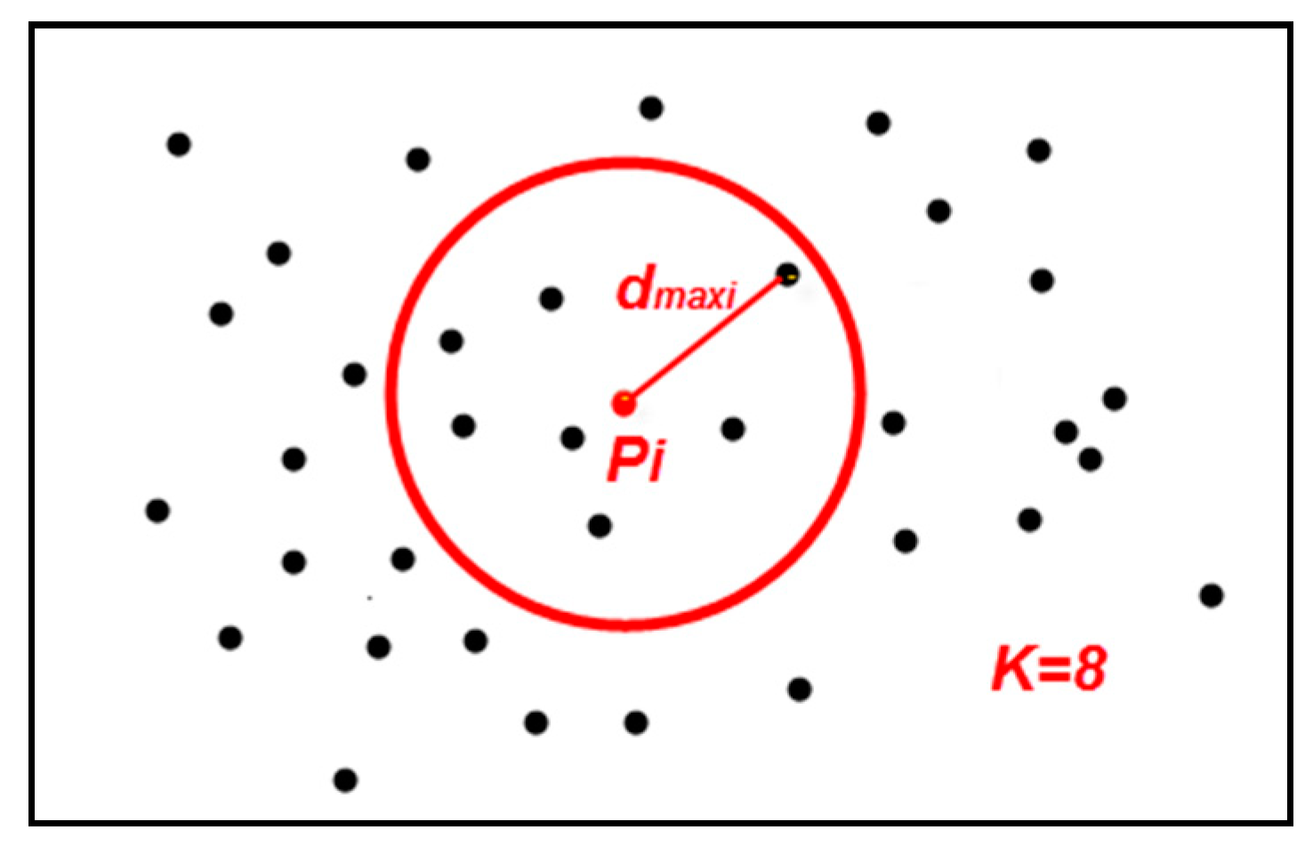
3.2.1. Definition
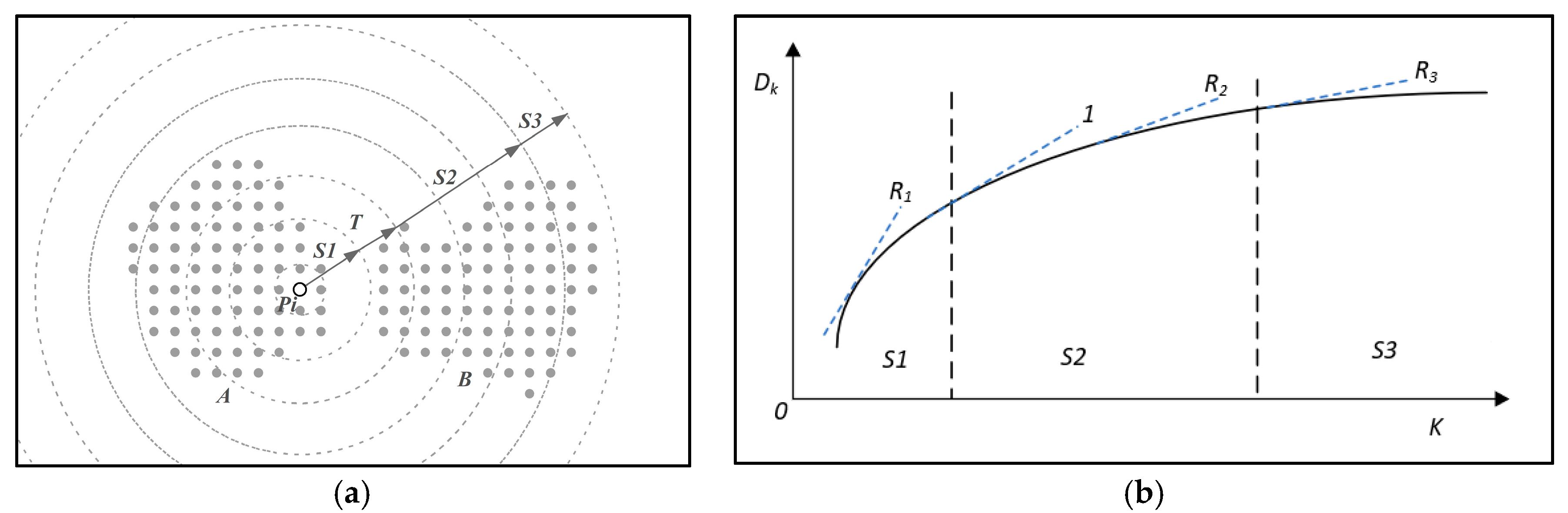
3.2.2. Analysis
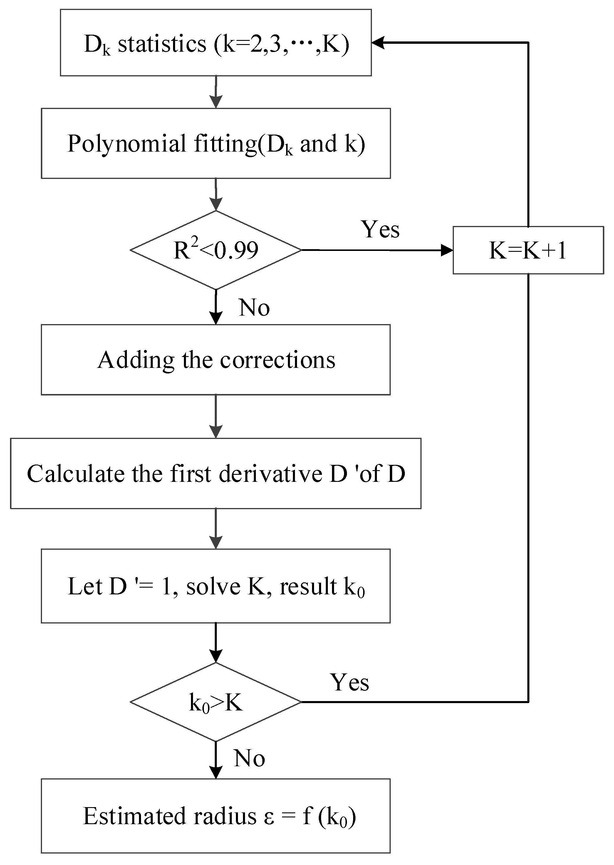
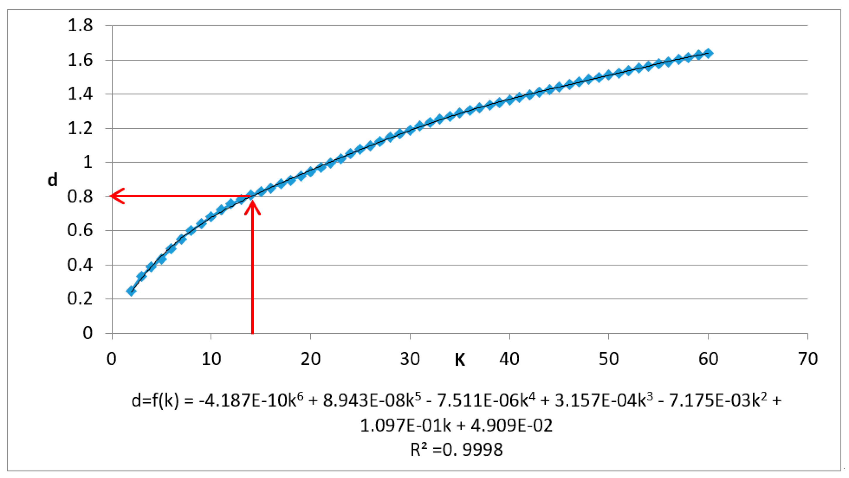
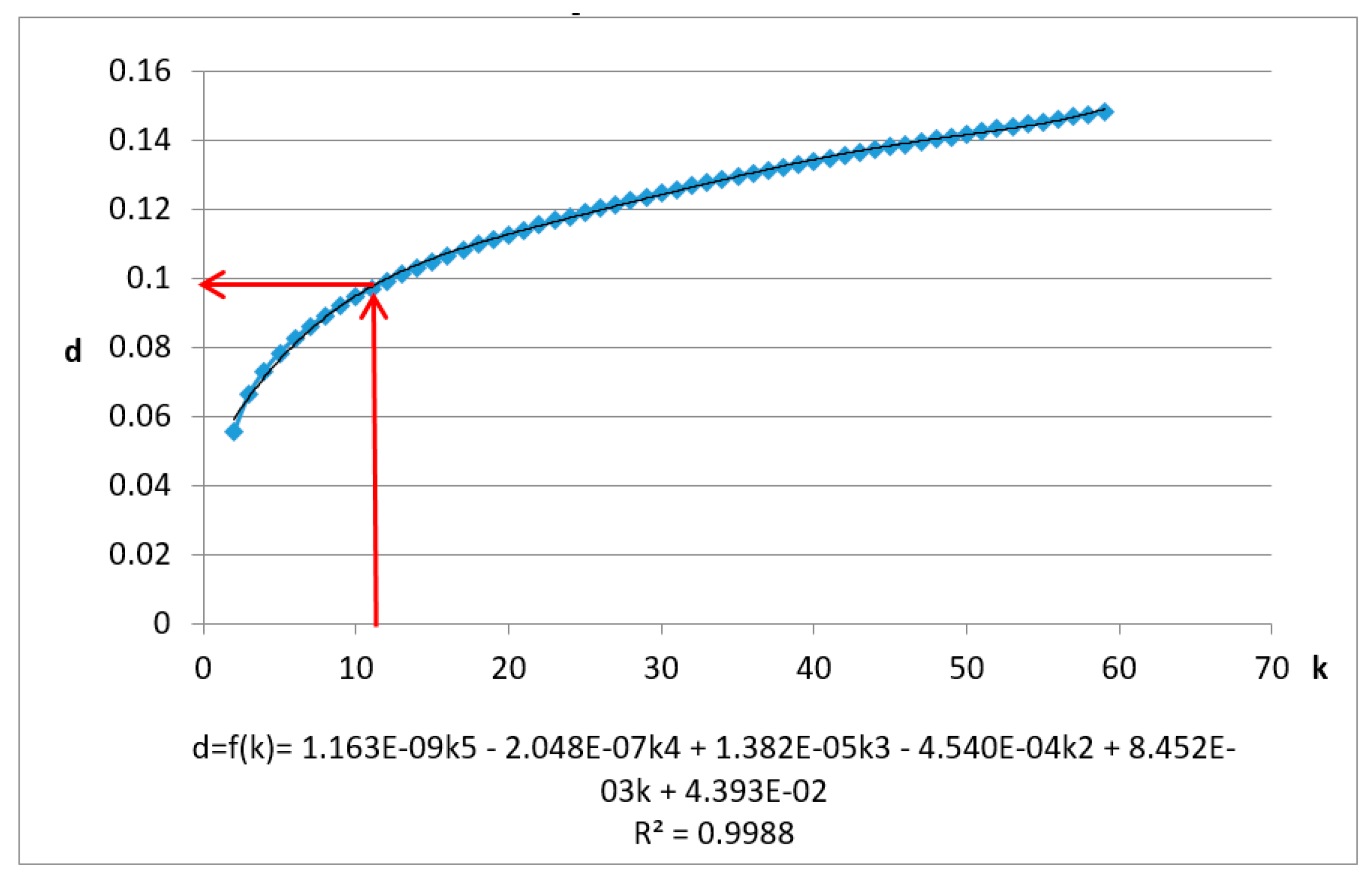
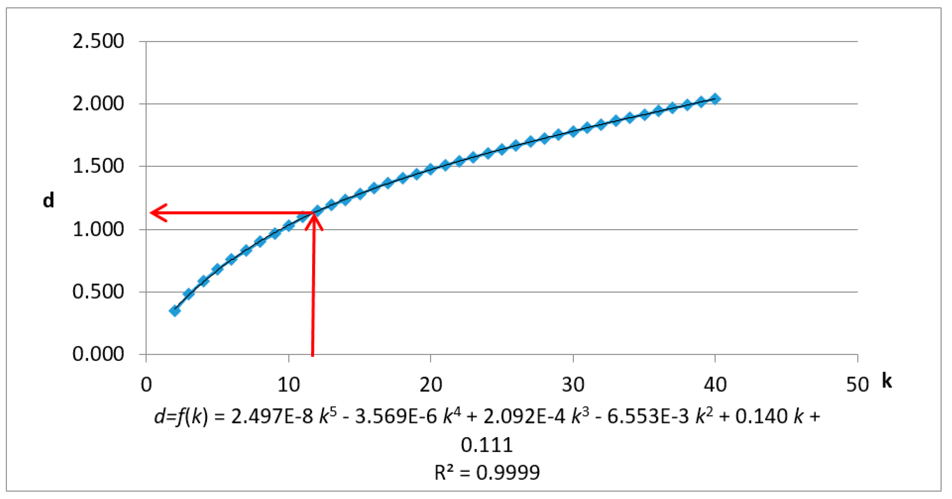
3.2.3. Method
- (1)
- Calculating Point Cloud P’s KNN mean max distance ()
- (2)
- Performing the polynomial fitting for the discrete function
- (3)
- Adding corrections
- (4)
- Deriving the first derivative of :
- (5)
- Calculating the estimated radius ε
3.3. Cluster Segmentation
3.3.1. Parameters
3.3.2. Clustering
| Algorithm 1 Improved DBSCAN Algorithm |
| Input: Dataset: P, minPts, ε, maxPts |
| Output: Clusters C |
| 1 Setting up an empty list of clusters C and an empty queue Q for the points that need to be checked |
| 2 for all, do |
| 3 if is processed then |
| 4 continue |
| 5 end |
| 6 add to the current queue Q |
| 7 for all do |
| 8 search for the set of point neighbors of in a sphere with radius ; |
| 9 for all |
| 10 if is not processed then |
| 11 add to Q |
| 12 end |
| 13 end |
| 14 end |
| 15 n = the point number of Q |
| 16 if then |
| 17 add Q to the list of clusters C |
| 18 for all do |
| 19 mark processed |
| 20 end |
| 21 reset Q to an empty list |
| 22 end |
| 23 end |
| 24 ReturnC |
3.4. Exporting Segmentation Results
4. Experimental Results and Analysis
4.1. Airborne LiDAR Data Experiments
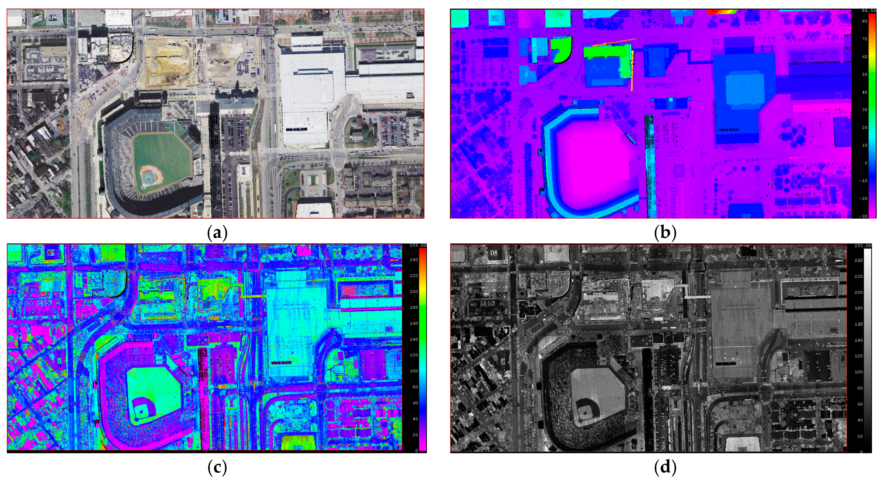
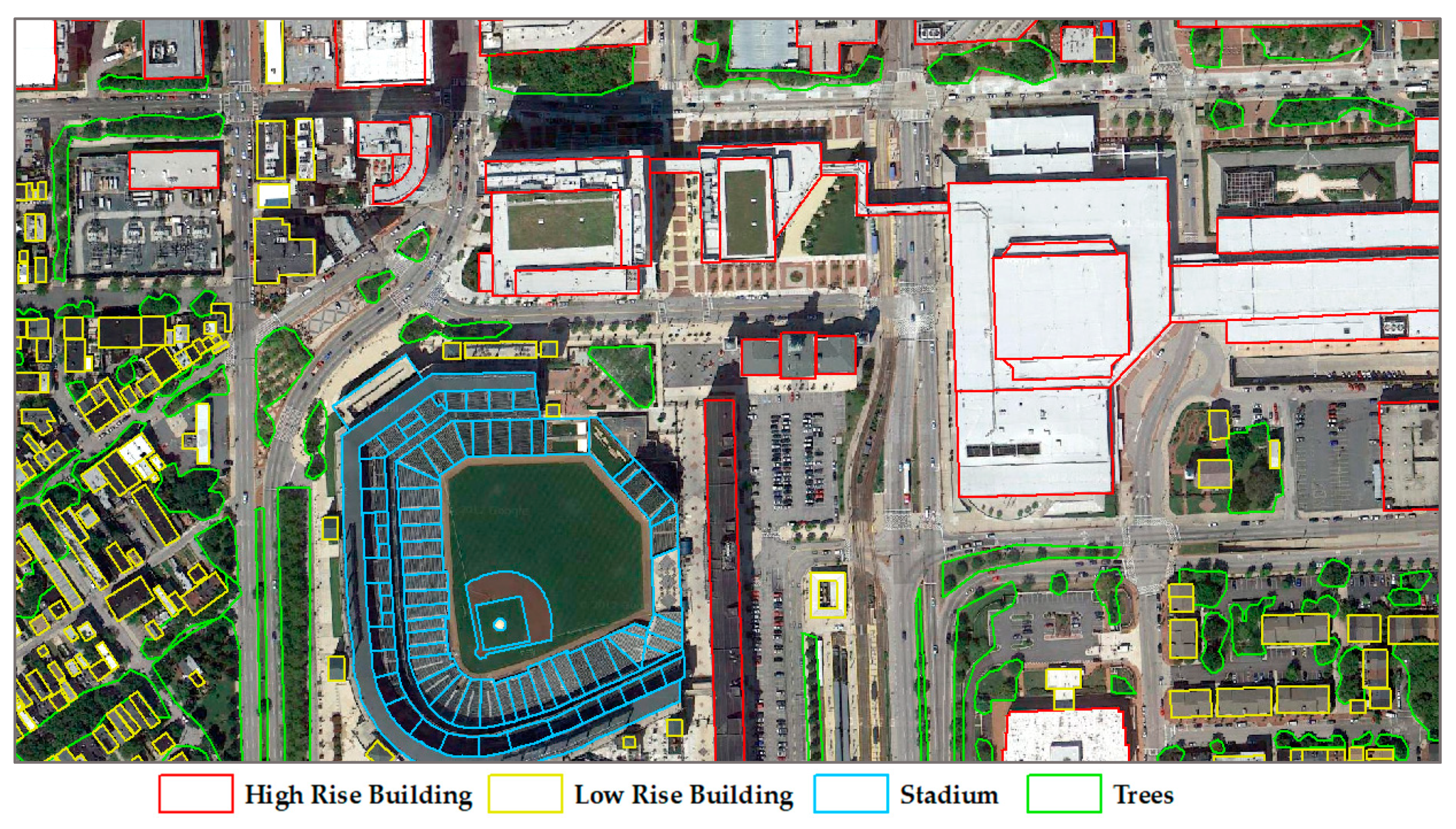
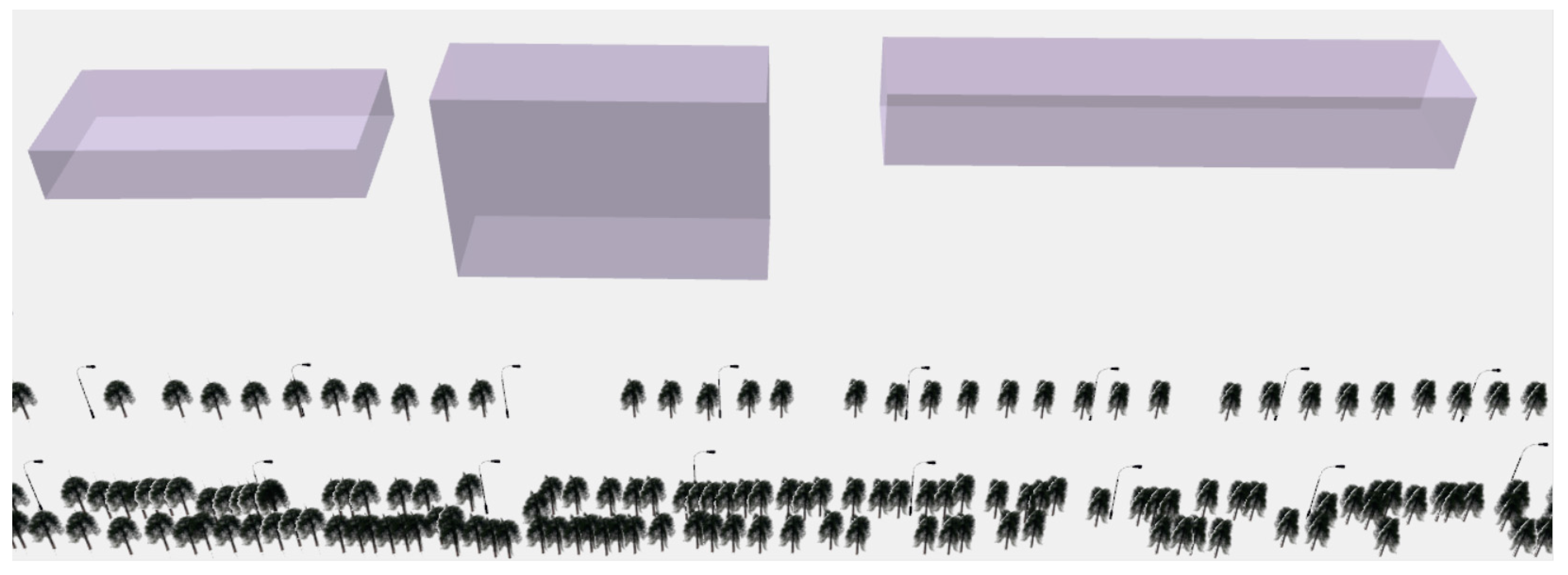
4.1.1. Study Area and Data Source
4.1.2. Using Spatial Information
Parameter Estimation
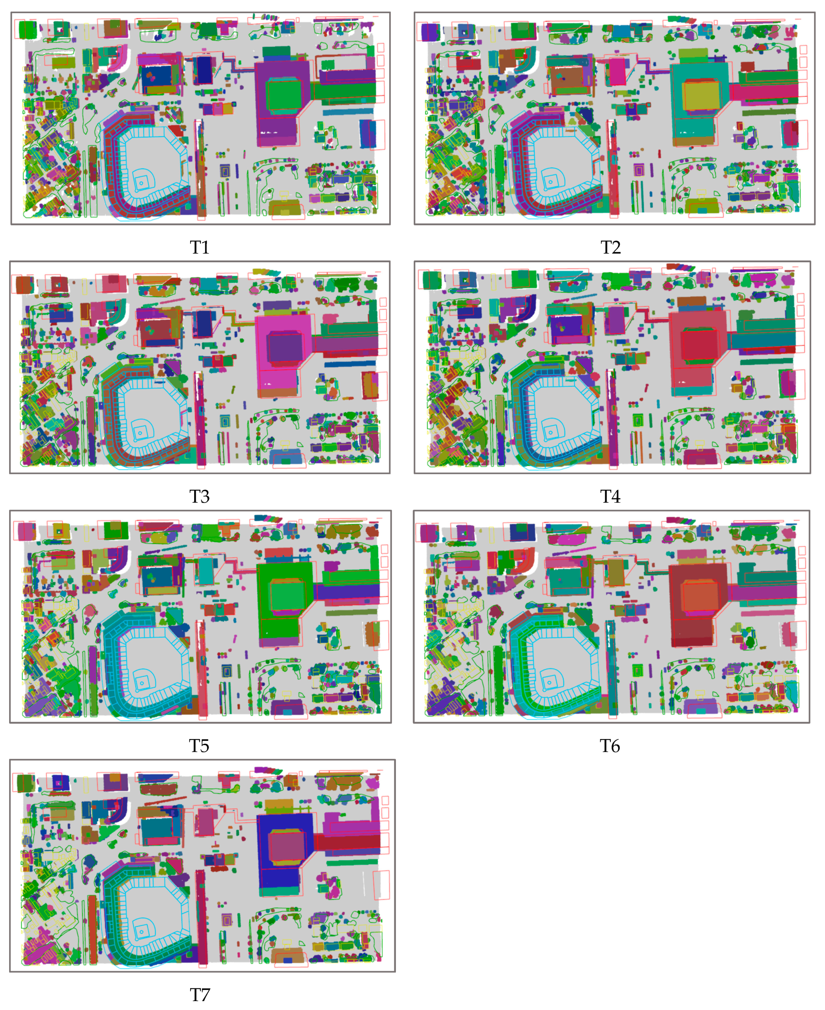
Clustering and Results
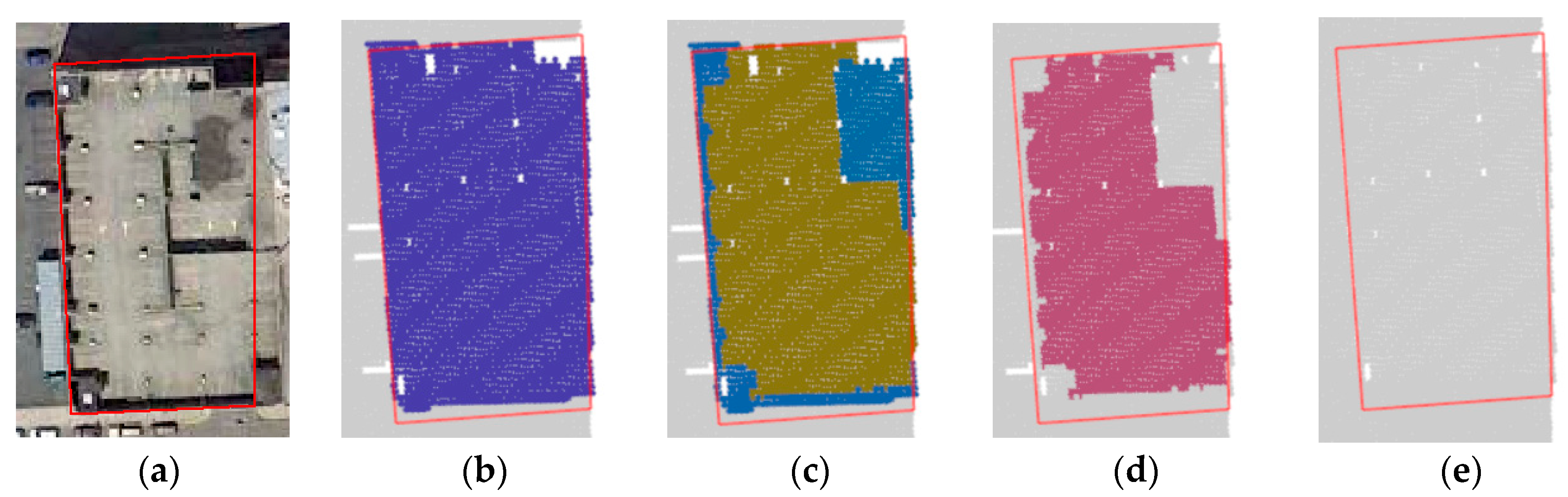
Accuracy Evaluation
4.1.3. Using Spatial and Color Information
Parameter Estimation
Clustering and Results
Accuracy Evaluation
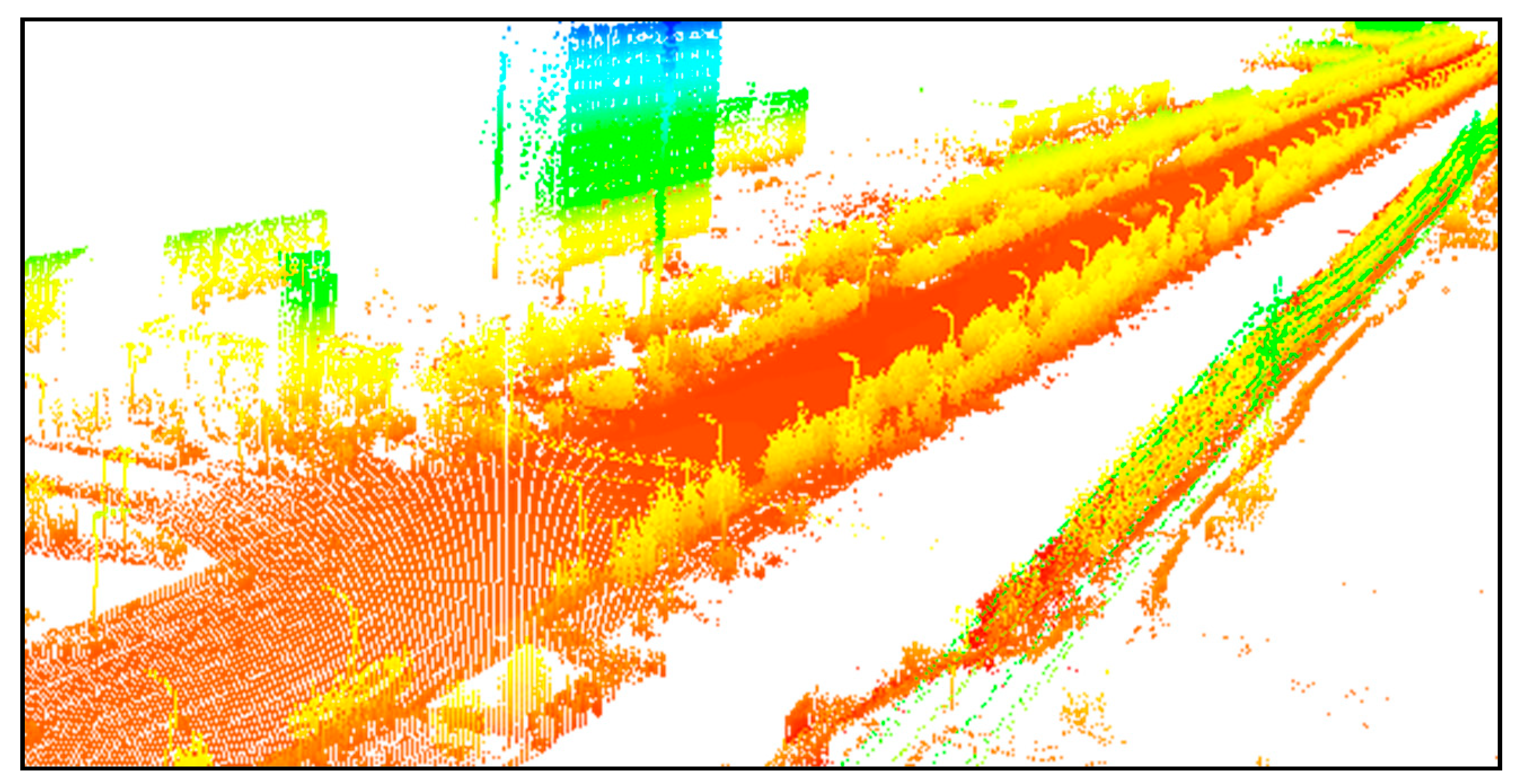
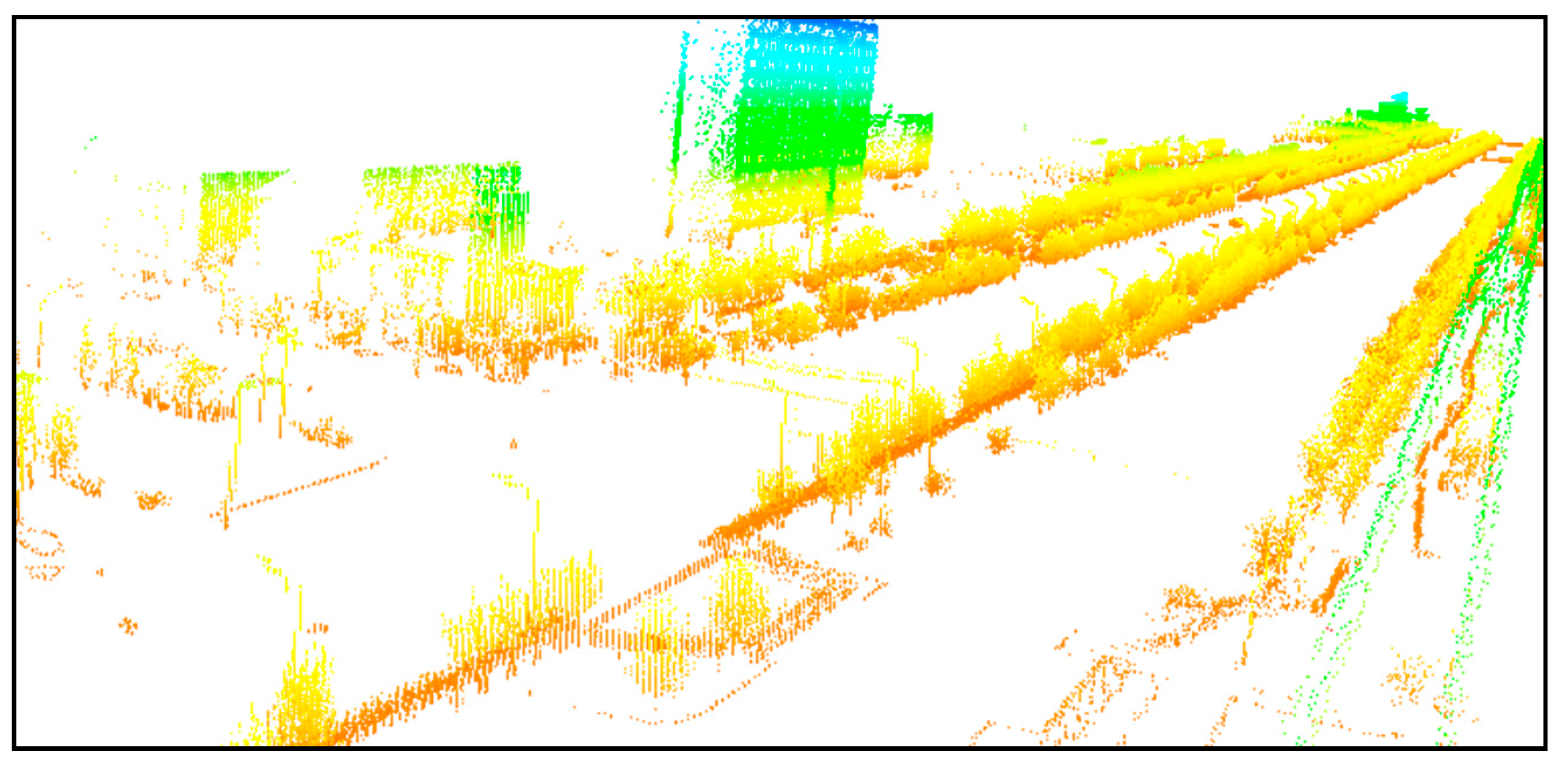
4.2. Mobile LiDAR Data Experiments
4.2.1. Study Area and Data Source
4.2.2. Using Spatial Information
Parameter Estimation
Clustering and Results
Accuracy Evaluation
4.3. Results
5. Conclusions
Author Contributions
Funding
Conflicts of Interest
References
- Akel, N.A.; Kremeike, K.; Filin, S.; Sester, M.; Doytsher, Y. Dense DTM generalization aided by roads extracted from LiDAR data. In Proceedings of the ISPRS WG III/3, III/4, V/3 Workshop “Laser scanning 2005”, Enschede, The Netherlands, 12–14 September 2005; pp. 54–59. [Google Scholar]
- Popescu, S.C.; Wynne, R.H. Seeing the trees in the forest: Using lidar and multispectral data fusion with local filtering and variable window size for estimating tree height. Photogramm. Eng. Remote Sens. 2004, 70, 589–604. [Google Scholar] [CrossRef]
- Bortolot, Z.J.; Wynne, R.H. Estimating forest biomass using small footprint LiDAR data: An individual tree-based approach that incorporates training data. ISPRS J. Photogramm. Remote Sens. 2005, 59, 342–360. [Google Scholar] [CrossRef]
- Hollaus, M.; Wagner, W.; Eberhöfer, C.; Karel, W. Accuracy of large-scale canopy heights derived from LiDAR data under operational constraints in a complex alpine environment. ISPRS J. Photogramm. Remote Sens. 2006, 60, 323–338. [Google Scholar] [CrossRef]
- Garcia-Alonso, M.; Ferraz, A.; Saatchi, S.S.; Casas, A.; Koltunov, A.; Ustin, S.; Ramirez, C.; Balzter, H. Estimating forest biomass from LiDAR data: A comparison of the raster-based and point-cloud data approach. In Proceedings of the AGU Fall Meeting, San Francisco, CA, USA, 14–18 December 2015. [Google Scholar]
- Murakami, H.; Nakagawa, K.; Hasegawa, H.; Shibata, T.; Iwanami, E. Change detection of buildings using an airborne laser scanner. ISPRS J. Photogramm. Remote Sens. 1999, 54, 148–152. [Google Scholar] [CrossRef]
- Gomes Pereira, L.; Janssen, L. Suitability of laser data for DTM generation: A case study in the context of road planning and design. ISPRS J. Photogramm. Remote Sens. 1999, 54, 244–253. [Google Scholar] [CrossRef]
- Clode, S.; Rottensteiner, F.; Kootsookos, P.; Zelniker, E. Detection and vectorisation of roads from lidar data. Photogramm. Eng. Remote Sens. 2006, 73, 517–535. [Google Scholar] [CrossRef]
- Quattoni, A.; Torralba, A. Recognizing indoor scenes. In Proceedings of the 2009 IEEE Conference on Computer Vision and Pattern Recognition, Miami, FL, USA, 20–25 June 2009. [Google Scholar]
- Inokuchi, H. Multi-Lidar System. U.S. Patent Application No. 20120092645A1, 19 April 2012. [Google Scholar]
- Ester, M.; Kriegel, H.P.; Sander, J.; Xu, X. A density-based algorithm for discovering clusters in large spatial databases with noise. In Proceedings of the 2nd International Conference on Knowledge Discovery and Data Mining, Portland, OR, USA, 2–4 August 1996. [Google Scholar]
- Ankerst, M.; Breunig, M.M.; Kriegel, H.P.; Sander, J. OPTICS: Ordering points to identify the clustering structure. In Proceedings of the 1999 ACM SIGMOD International Conference on Management of Data, Philadelphia, PA, USA, 31 May–3 June 1999; pp. 49–60. [Google Scholar]
- Hinneburg, A.; Gabriel, H.-H. DENCLUE 2.0: Fast Clustering Based on Kernel Density Estimation. In Intelligent Data Analysis VII, Proceedings of the 7th International Symposium on Intelligent Data Analysis, IDA 2007, Ljubljana, Slovenia, 6–8 September 2007; Berthold, M.R., Shawe-Taylor, J., Lavrač, N., Eds.; Springer: Berlin, Germany, 2007; pp. 70–80. [Google Scholar]
- Han, J.; Kamber, M. Density-Based Methods. In Data Mining: Concepts and Technique; Morgan Kaufmann Publishers: Burlington, MA, USA, 2006; Chapter 7; pp. 418–422. [Google Scholar]
- Ghosh, S.; Lohani, B. Heuristical Feature Extraction from LIDAR Data and Their Visualization. ISPRS—Int. Arch. Photogramm. Remote Sens. Spat. Inf. Sci. 2012, 38, 13–18. [Google Scholar] [CrossRef]
- Schubert, E.; Sander, J.; Ester, M.; Kriegel, H.P.; Xu, X. DBSCAN Revisited, Revisited: Why and How You Should (Still) Use DBSCAN. ACM Trans. Database Syst. 2017, 42, 1–21. [Google Scholar] [CrossRef]
- Sander, J.; Ester, M.; Kriegel, H.P.; Xu, X. Density-Based Clustering in Spatial Databases: The Algorithm GDBSCAN and Its Applications. Data Min. Knowl. Discov. 1998, 2, 169–194. [Google Scholar] [CrossRef]
- Daszykowski, M.; Walczak, B.; Massart, D.L. Looking for natural patterns in data: Part 1. Density-based approach. Chemom. Intell. Lab. Syst. 2001, 56, 83–92. [Google Scholar] [CrossRef]
- Dua, D.; Karra Taniskidou, E. UCI Machine Learning Repository. University of California, School of Information and Computer Science: Irvine, CA, USA. 2017. Available online: http://archive.ics.uci.edu/ml (accessed on 3 January 2019).
- Gan, J.; Tao, Y. DBSCAN Revisited: Mis-Claim, Un-Fixability, and Approximation. In Proceedings of the 2015 ACM SIGMOD International Conference on Management of Data, Melbourne, Australia, 31 May–4 June 2015; pp. 519–530. [Google Scholar]
- Hubert, L.; Arabie, P. Comparing partitions. J. Classif. 1985, 2, 193–218. [Google Scholar] [CrossRef]
- Ghosh, S.; Lohani, B. Mining lidar data with spatial clustering algorithms. Int. J. Remote Sens. 2013, 34, 5119–5135. [Google Scholar] [CrossRef]
- Lari, Z.; Habib, A. Alternative methodologies for the estimation of local point density index: Moving towards adaptive LiDAR data processing. Int. Arch. Photogramm. Remote Sens. Spat. Inf. Sci. 2012, 39, 127–132. [Google Scholar] [CrossRef]
- Biosca, J.M.; Lerma, J.L. Unsupervised robust planar segmentation of terrestrial laser scanner point clouds based on fuzzy clustering methods. ISPRS J. Photogramm. Remote. Sens. 2008, 63, 84–98. [Google Scholar] [CrossRef]
- Filin, S. Surface clustering from airborne laser scanning data. Int. Arch. Photogramm. Remote Sens. Spat. Inf. Sci. 2002, 34, 119–124. [Google Scholar]
- Jiang, B. Extraction of Spatial Objects from Laser-Scanning data using a clustering technique. In Proceedings of the XXth ISPRS Congress, Istanbul, Turkey, 12–13 July 2004. [Google Scholar]
- Morsdorf, F.; Meier, E.; Allgöwer, B.; Nüesch, D. Clustering in airborne laser scanning raw data for segmentation of single trees. Int. Arch. Photogramm. Remote Sens. Spat. Inf. Sci. 2003, 34, W13. [Google Scholar]
- Roggero, M. Object segmentation with region growing and principal component analysis. Int. Arch. Photogramm. Remote Sens. Spat. Inf. Sci. 2002, 34, 289–294. [Google Scholar]
- Crosilla, F.; Visintini, D.; Sepic, F. A statistically proven automatic curvature based classification procedure of laser points. In Proceedings of the XXI ISPRS Congress, Beijing, China, 3–11 July 2008. [Google Scholar]
- Jain, A.K.; Duin, R.P.W.; Mao, J. Statistical pattern recognition: A review. IEEE Trans. Pattern Anal. Mach. Intell. 2000, 22, 4–37. [Google Scholar] [CrossRef]
- Ballard, D.H. Generalizing the Hough transform to detect arbitrary shapes. Pattern Recognit. 1981, 13, 111–122. [Google Scholar] [CrossRef]
- Tarsha-Kurdi, F.; Tania, L.; Pierre, G. Hough-transform and extended ransac algorithms for automatic detection of 3d building roof planes from lidar data. Int. Arch. Photogramm. Remote Sens. Spat. Inf. Syst. 2007, 36, 407–412. [Google Scholar]
- Fischler, M.; Bolles, R. Random sample consensus: A paradigm for model fitting with applications to image analysis and automated cartography. Commun. ACM 1981, 24, 381–395. [Google Scholar] [CrossRef]
- Hoffman, R.; Jain, A.K. Segmentation and classification of range images. IEEE Trans. Pattern Anal. Mach. Intell. 1987, 5, 608–620. [Google Scholar] [CrossRef]
- Yang, B.; Huang, R.; Dong, Z.; Zang, Y.; Li, J. Two-step adaptive extraction method for ground points and breaklines from lidar point clouds. ISPRS J. Photogramm. Remote Sens. 2016, 119, 373–389. [Google Scholar] [CrossRef]
- Maas, H.G.; Vosselman, G. Two algorithms for extracting building models from raw laser altimetry data. ISPRS J. Photogramm. Remote. Sens. 1999, 54, 153–163. [Google Scholar] [CrossRef]
- Riveiro, B.; González-Jorge, H.; Martínez-Sánchez, J.; Díaz-Vilariño, L.; Arias, P. Automatic detection of zebra crossings from mobile LiDAR data. Opt. Laser Technol. 2015, 70, 63–70. [Google Scholar] [CrossRef]
- Neidhart, H.; Sester, M. Extraction of building ground plans from Lidar data. Int. Arch. Photogramm. Remote Sens. Spat. Inf. Sci. 2008, 37, 405–410. [Google Scholar]
- Woo, H.; Kang, E.; Wang, S.; Lee, K.H. A new segmentation method for point cloud data. Int. J. Mach. Tools Manuf. 2002, 42, 167–178. [Google Scholar] [CrossRef]
- Su, Y.-T.; Bethel, J.; Hu, S. Octree-based segmentation for terrestrial LiDAR point cloud data in industrial applications. ISPRS J. Photogramm. Remote Sens. 2016, 113, 59–74. [Google Scholar] [CrossRef]
- Vo, A.V.; Truong-Hong, L.; Laefer, D.F.; Bertolotto, M. Octree-based region growing for point cloud segmentation. ISPRS J. Photogramm. Remote. Sens. 2015, 104, 88–100. [Google Scholar] [CrossRef]
- Boulaassal, H.; Landes, T.; Grussenmeyer, P.; Tarsha-Kurdi, F. Automatic segmentation of building facades using terrestrial laser data. In Proceedings of the ISPRS Workshop on Laser Scanning 2007 and SilviLaser, Espoo, Finland, 12–14 September 2007; Volume XXXVI, pp. 65–70. [Google Scholar]
- Schnabel, R.; Wahl, R.; Klein, R. Efficient RANSAC for Point-Cloud Shape Detection. In Computer Graphics Forum; Wiley Online Library: Hoboken, NJ, USA, 2007. [Google Scholar]
- Awwad, T.M.; Zhu, Q.; Du, Z.; Zhang, Y. An improved segmentation approach for planar surfaces from unstructured 3D point clouds. Photogramm. Rec. 2010, 25, 5–23. [Google Scholar] [CrossRef]
- Schwalbe, E.; Maas, H.-G.; Seidel, F. 3D building model generation from airborne laser scanner data using 2D GIS data and orthogonal point cloud projections. In Proceedings of the ISPRS WG III/3, III/4, Enschede, The Netherlands, 12–14 September 2005; Volume 3, pp. 12–14. [Google Scholar]
- Moosmann, F.; Pink, O.; Stiller, C. Segmentation of 3D lidar data in non-flat urban environments using a local convexity criterion. In Proceedings of the 2009 IEEE Intelligent Vehicles Symposium, Xi’an, China, 3–5 June 2009. [Google Scholar]
- Douillard, B.; Douillard, B.; Underwood, J.; Kuntz, N.; Vlaskine, V.; Quadros, A.; Morton, P.; Frenkel, A. On the segmentation of 3D LIDAR point clouds. In Proceedings of the 2011 IEEE International Conference on Robotics and Automation, Shanghai, China, 9–13 May 2011. [Google Scholar]
- Besl, P.J.; Jain, R.C. Segmentation through variable-order surface fitting. IEEE Trans. Pattern Anal. Mach. Intell. 1988, 10, 167–192. [Google Scholar] [CrossRef]
- Rabbani, T. Automatic Reconstruction of Industrial Installations Using Point Clouds and Images; NCG: Delft, The Netherlands, 2006. [Google Scholar]
- Hofmann, A. Analysis of TIN-structure parameter spaces in airborne laser scanner data for 3-D building model generation. Int. Arch. Photogramm. Remote Sens. Spat. Inf. Sci. 2004, 35, 302–307. [Google Scholar]
- Wang, C.-K.; Hsu, P.-H. Building Extraction from LiDAR Data Using Wavelet Analysis. In Proceedings of the 27th Asian Conference on Remote Sensing, Ulaanbaatar, Mongolia, 9–13 October 2006. [Google Scholar]
- Höfle, B.; Hollaus, M.; Hagenauer, J. Urban vegetation detection using radiometrically calibrated small-footprint full-waveform airborne LiDAR data. ISPRS J. Photogramm. Remote Sens. 2012, 67, 134–147. [Google Scholar] [CrossRef]
- Niemeyer, J.; Rottensteiner, F.; Soergel, U. Contextual classification of lidar data and building object detection in urban areas. ISPRS J. Photogramm. Remote Sens. 2014, 87, 152–165. [Google Scholar] [CrossRef]
- Anguelov, D.; Taskarf, B.; Chatalbashev, V.; Koller, D.; Gupta, D.; Heitz, G.; Ng, A. Discriminative learning of markov random fields for segmentation of 3d scan data. In Proceedings of the IEEE Computer Society Conference on Computer Vision and Pattern Recognition, San Diego, CA, USA, 20–25 June 2005. [Google Scholar]
- Triebel, R.; Kersting, K.; Burgard, W. Robust 3D scan point classification using associative Markov networks. In Proceedings of the IEEE International Conference on Robotics and Automation, Orlando, FL, USA, 15–19 May 2006. [Google Scholar]
- Meng, X.; Currit, N.; Zhao, K. Ground Filtering Algorithms for Airborne LiDAR Data: A Review of Critical Issues. Remote Sens. 2010, 2, 833–860. [Google Scholar] [CrossRef]
- Rusu, R.B. Semantic 3D Object Maps for Everyday Manipulation in Human Living Environments. KI-Künstliche Intell. 2010, 24, 345–348. [Google Scholar] [CrossRef]
- Campello, R.J.G.B.; Moulavi, D.; Sander, J. Density-Based Clustering Based on Hierarchical Density Estimates. In Lecture Notes in Computer Science; Pei, J., Tseng, V.S., Cao, L., Motoda, H., Xu, G., Eds.; Advances in Knowledge Discovery and Data Mining; Springer: Berlin, Germany, 2013; Volume 7819. [Google Scholar]
- Hoover, A.; Jean-Baptiste, G.; Jiang, X.; Flynn, P.J.; Bunke, H.; Goldgof, D.B.; Fisher, R.B. An experimental comparison of range image segmentation algorithms. IEEE Trans. Pattern Anal. Mach. Intell. 1996, 18, 673–689. [Google Scholar] [CrossRef]


| Class | Name | T1 | T2 | T3 | T4 | T5 | T6 | T7 |
|---|---|---|---|---|---|---|---|---|
| Inputs | ε | 0.6 | 0.7 | 0.8 | 0.8114 | 0.9 | 1.0 | 1.1 |
| Results | Run Time (s) | 20.0 | 22.2 | 22.2 | 22.0 | 22.8 | 26.5 | 32.8 |
| No. of Clusters | 901 | 828 | 729 | 728 | 660 | 577 | 486 | |
| Noise Ratio (%) | 8.8 | 5.8 | 4.1 | 3.9 | 3.0 | 2.3 | 1.7 |
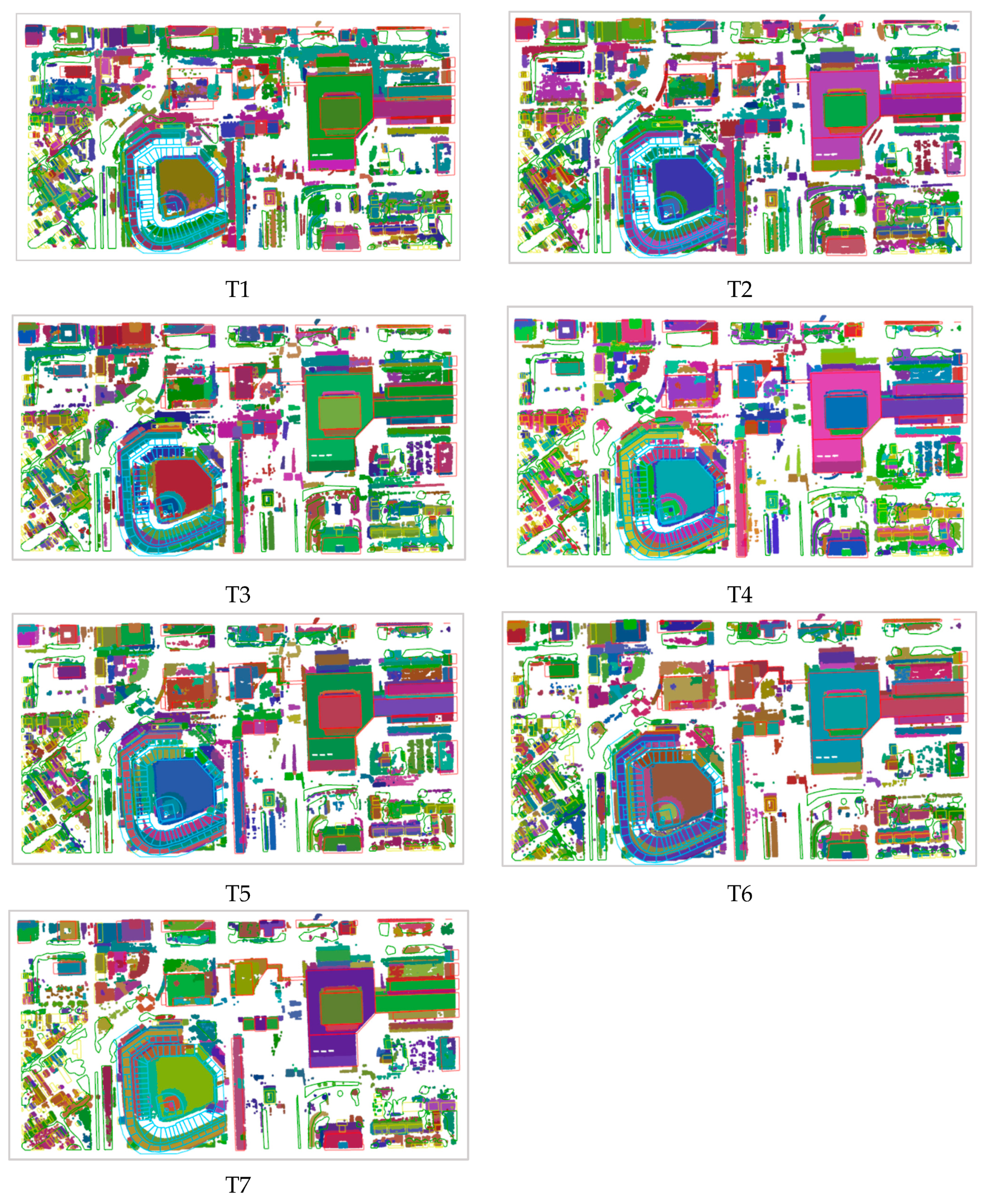
| Test | ε | Correct Detection | Under-Segmentation | Over-Segmentation | Missed | Accuracy |
|---|---|---|---|---|---|---|
| T1 | 0.6 | 149 | 40 | 81 | 63 | 45% |
| T2 | 0.7 | 176 | 36 | 65 | 56 | 53% |
| T3 | 0.8 | 233 | 17 | 36 | 47 | 70% |
| T4 | 0.8114 | 251 | 21 | 15 | 46 | 75% |
| T5 | 0.9 | 201 | 33 | 36 | 63 | 60% |
| T6 | 1.0 | 210 | 29 | 26 | 68 | 63% |
| T7 | 1.1 | 182 | 51 | 7 | 93 | 55% |
| Class | Name | T1 | T2 | T3 | T4 | T5 | T6 | T7 |
|---|---|---|---|---|---|---|---|---|
| Inputs | ε | 0.07 | 0.08 | 0.09 | 0.097 | 0.1 | 0.11 | 0.12 |
| Results | Run Time (s) | 52.1 | 65.2 | 82.0 | 91.6 | 105.4 | 133.3 | 166.3 |
| No. of Clusters | 635 | 632 | 570 | 504 | 498 | 412 | 340 | |
| Noise Ratio (%) | 31.0 | 23.6 | 18.0 | 14.4 | 13.2 | 9.3 | 6.1 |
| Test | ε | Correct Detection | Under-Segmentation | Over-Segmentation | Missed | Accuracy |
|---|---|---|---|---|---|---|
| T1 | 0.07 | 157 | 53 | 73 | 50 | 47% |
| T2 | 0.08 | 178 | 58 | 58 | 39 | 53% |
| T3 | 0.09 | 236 | 27 | 48 | 22 | 71% |
| T4 | 0.097 | 247 | 24 | 43 | 19 | 74% |
| T5 | 0.10 | 236 | 25 | 40 | 32 | 71% |
| T6 | 0.11 | 192 | 65 | 25 | 51 | 58% |
| T7 | 0.12 | 173 | 90 | 8 | 62 | 52% |
| Class | Name | T1 | T2 | T3 | T4 | T5 | T6 | T7 |
|---|---|---|---|---|---|---|---|---|
| Inputs | ε | 0.5 | 0.8 | 1.1 | 1.14686 | 1.2 | 1.5 | 1.7 |
| Results | Run Time (s) | 3.5 | 6.3 | 9.4 | 12.8 | 13.7 | 14.8 | 18.5 |
| Number of clusters | 186 | 663 | 619 | 611 | 592 | 459 | 385 | |
| Noise Ratio (%) | 84.1 | 27.9 | 15.9 | 14.4 | 12.7 | 8.5 | 6.5 |
| Test | ε | Correct Detection | Under-Segmentation | Over-Segmentation | Missed | Accuracy |
|---|---|---|---|---|---|---|
| T1 | 0.5 | 48 | 14 | 4 | 846 | 5% |
| T2 | 0.8 | 394 | 93 | 3 | 422 | 43% |
| T3 | 1.1 | 598 | 51 | 23 | 240 | 66% |
| T4 | 1.14686 | 645 | 44 | 15 | 208 | 71% |
| T5 | 1.2 | 579 | 131 | 3 | 199 | 63% |
| T6 | 1.5 | 382 | 338 | 4 | 188 | 42% |
| T7 | 1.7 | 271 | 455 | 3 | 183 | 30% |
© 2019 by the authors. Licensee MDPI, Basel, Switzerland. This article is an open access article distributed under the terms and conditions of the Creative Commons Attribution (CC BY) license (http://creativecommons.org/licenses/by/4.0/).
Share and Cite
Wang, C.; Ji, M.; Wang, J.; Wen, W.; Li, T.; Sun, Y. An Improved DBSCAN Method for LiDAR Data Segmentation with Automatic Eps Estimation. Sensors 2019, 19, 172. https://doi.org/10.3390/s19010172
Wang C, Ji M, Wang J, Wen W, Li T, Sun Y. An Improved DBSCAN Method for LiDAR Data Segmentation with Automatic Eps Estimation. Sensors. 2019; 19(1):172. https://doi.org/10.3390/s19010172
Chicago/Turabian StyleWang, Chunxiao, Min Ji, Jian Wang, Wei Wen, Ting Li, and Yong Sun. 2019. "An Improved DBSCAN Method for LiDAR Data Segmentation with Automatic Eps Estimation" Sensors 19, no. 1: 172. https://doi.org/10.3390/s19010172
APA StyleWang, C., Ji, M., Wang, J., Wen, W., Li, T., & Sun, Y. (2019). An Improved DBSCAN Method for LiDAR Data Segmentation with Automatic Eps Estimation. Sensors, 19(1), 172. https://doi.org/10.3390/s19010172