Realistic Indoor Radio Propagation for Sub-GHz Communication


Abstract
1. Introduction
2. Related Literature
- Ray-based algorithms that make it possible to trace a set of rays in the modeled environment until a specific location. Every ray that is either traced or launched from a transmitter location and is able to reflect, refract, or diffract in the environment by using the Geometric Optics (GO) theory and the Uniform Theory of Diffraction (UTD). Ray-based methods enable the visibility of every path from transmitter to receiver, which gives researchers a better understanding of the underlying phenomena within the frequency spectrum. On one hand, the literature states an image-based solution, which traces all ray paths from a receiver location towards a transmitter location [10,16,17]. On the other hand, a ray-launching solution makes it possible to launch many different rays according to a specific antenna radiation pattern. Since both solutions are providing a good accuracy, they are widely being applied for either outdoor and indoor coverage simulations [13].
- Finite Difference Time Domain (FDTD) and Method of Moments (MoM) models are solutions that solve the Maxwell’s equations in both time and frequency domains [18,19]. All of these deterministic propagation loss model solutions use a grid-based environment model, which can define a 2D or a 3D environment model, to compute at every cell the electrical field relative to the time according to the differential or integral method. The different wave propagation phenomena make such an algorithm very complex on one side, while these algorithms obtain the optimal accuracy and precision for the given environment model relative to the resolution of the obtained environment [6].
3. Environment Modeling
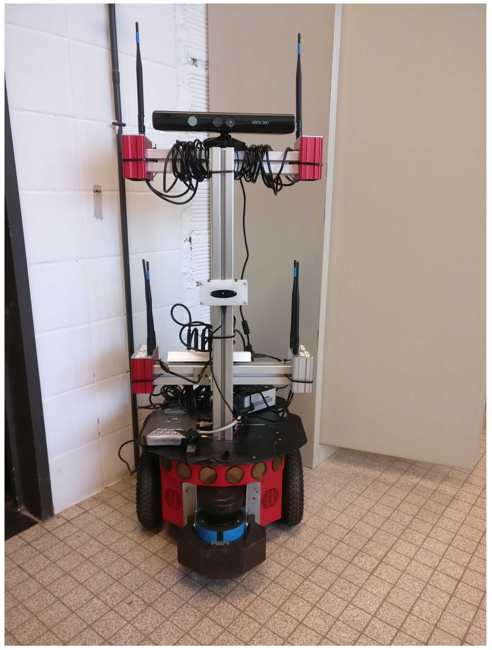
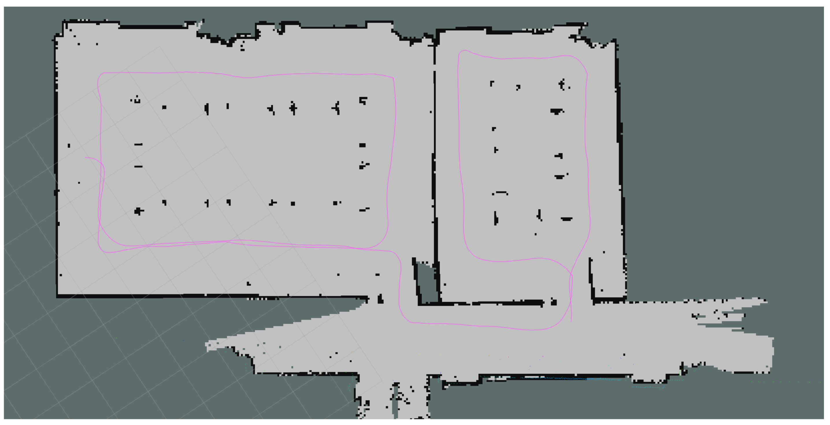
3.1. SLAM
3.2. Robot
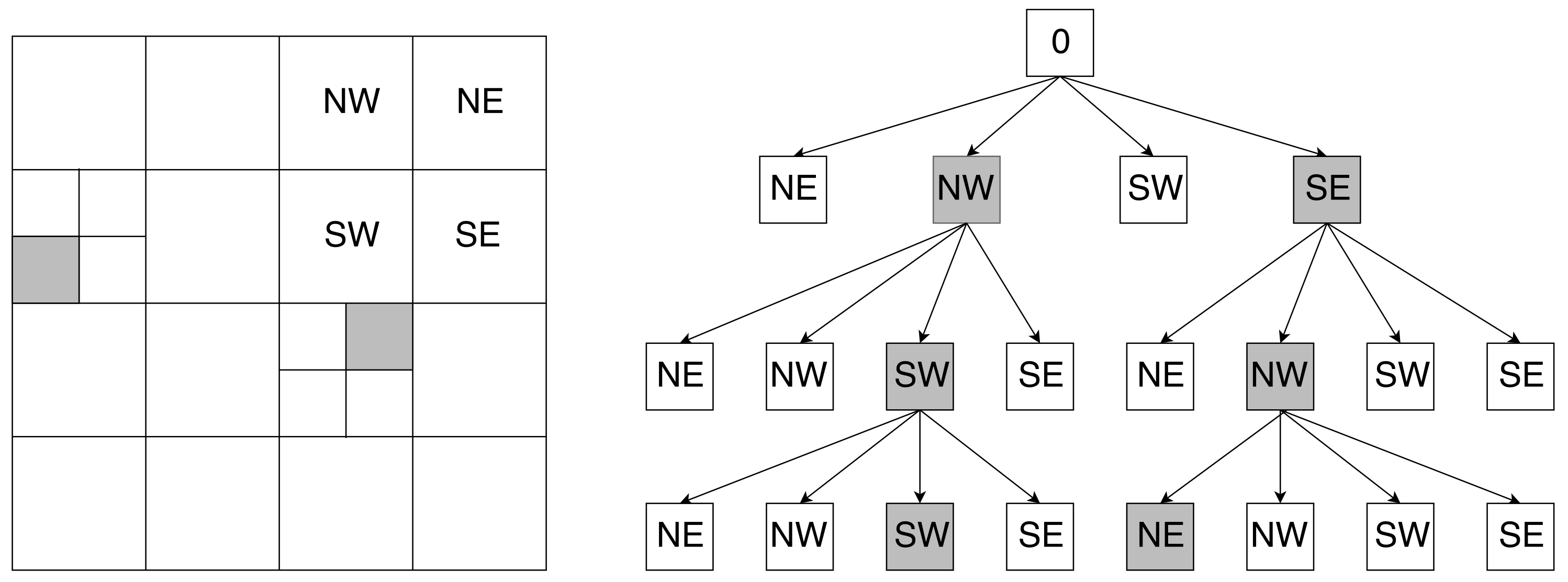
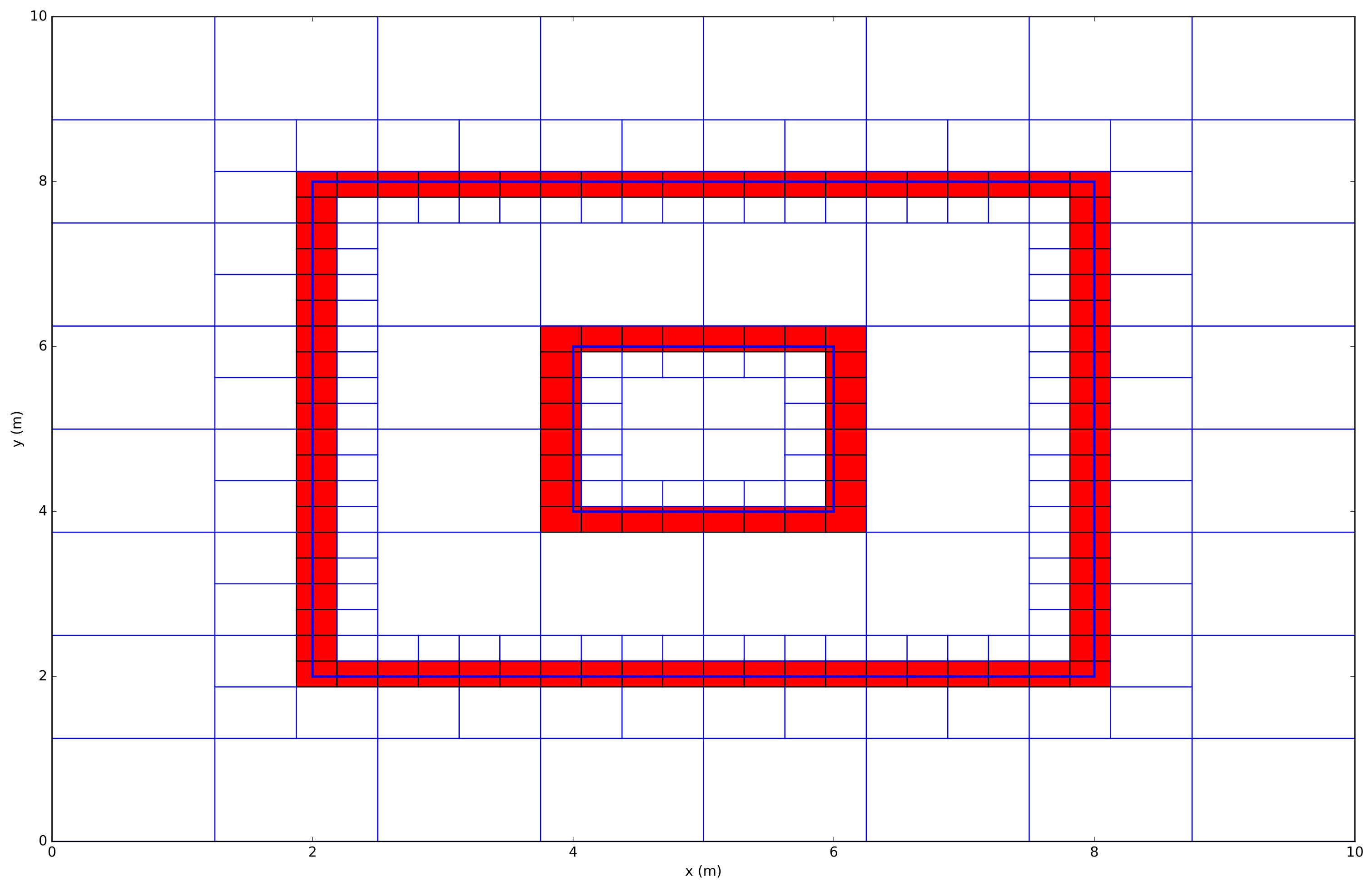
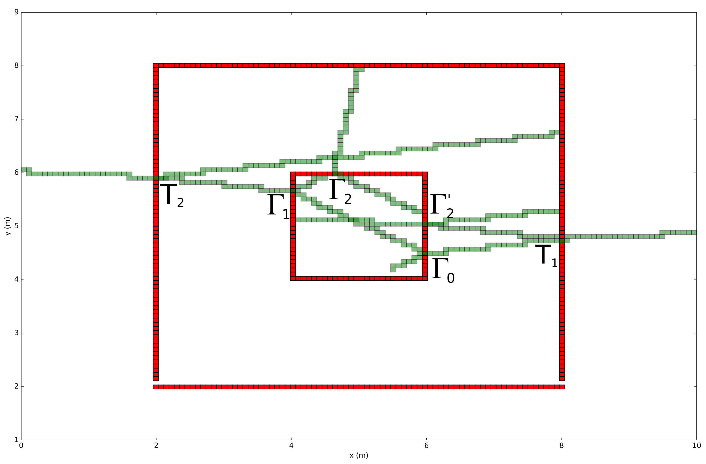
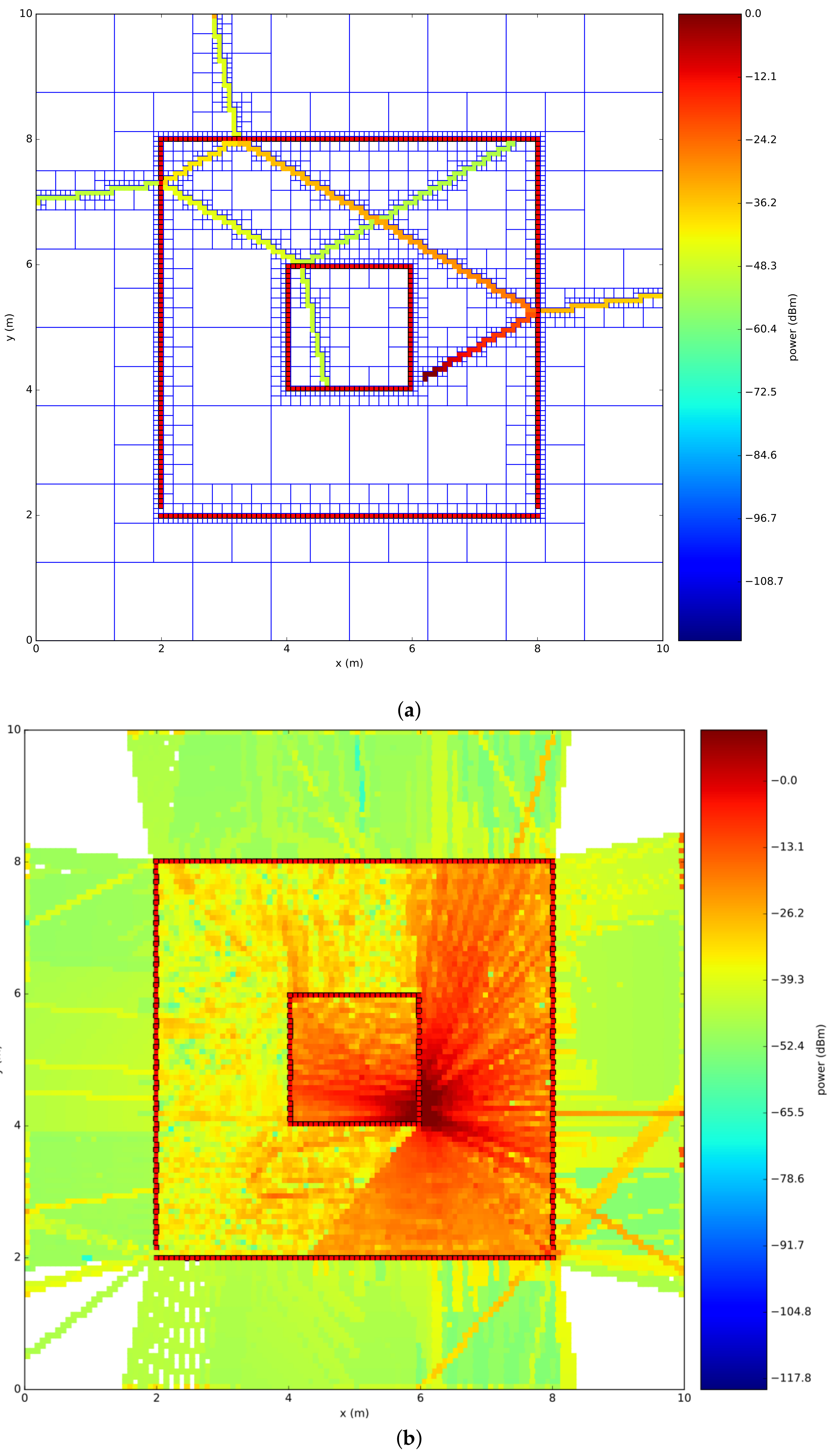
3.3. Quadtree
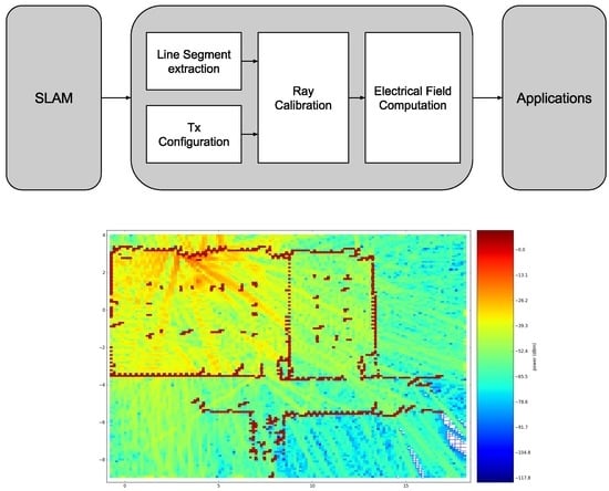
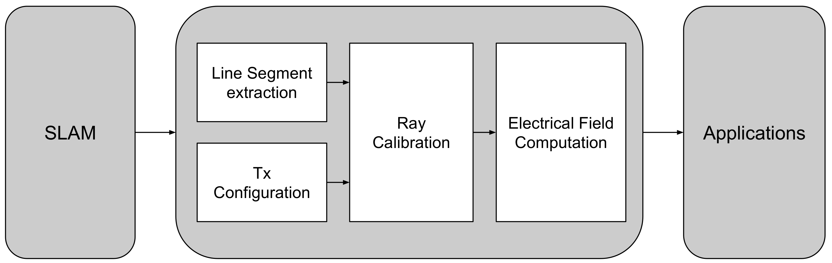
4. Ray Launching Propagation Loss Model
- Line-segment extraction: This method, explained in Section 4.1, contributes to the extraction of line segments and the segmentation of walls and objects by applying a region growing connected component labeling algorithm on top of the Quadtree that contains points.
- Device configuration: As described in Section 4.2, each device holds a simulation configuration that contains necessary parameters.
- Ray Calibration: During this process, which is explained in Section 4.3, every ray will be launched according to a transmitter device configuration and will reflect and refract in the environment model that is defined by a Quadtree or an Octree. Because each environment model is modeled with a maximum resolution level, every ray will be launched according to that level. In order to increase the performance of this process, all rays are processed in a parallel fashion. The result of this ray calibration method is a list for every ray that exists of all visited cells. This list contains the total distance from transmitter to receiver together with the Fresnel reflection coefficients. Besides the fact that every ray is calibrated towards the maximum number of reflections and refractions, all binary addresses of the visited cells were stored in the object. This enables the usability to re-use this calibration data in order to simulate the signal strength for a different frequency or to apply a simulation where a subset of the rays is used, which makes it scalable and efficient to apply a benchmark.
- Electrical Field Computation: Due to the previous calibration process, all parameters in order to compute the electrical field at every visited cell for each ray are known. Section 4.4 computes for each visited cell the electrical field related to these parameters. As a result, a coverage map can be created by computing the sum of all electrical fields at every cell that was visited.
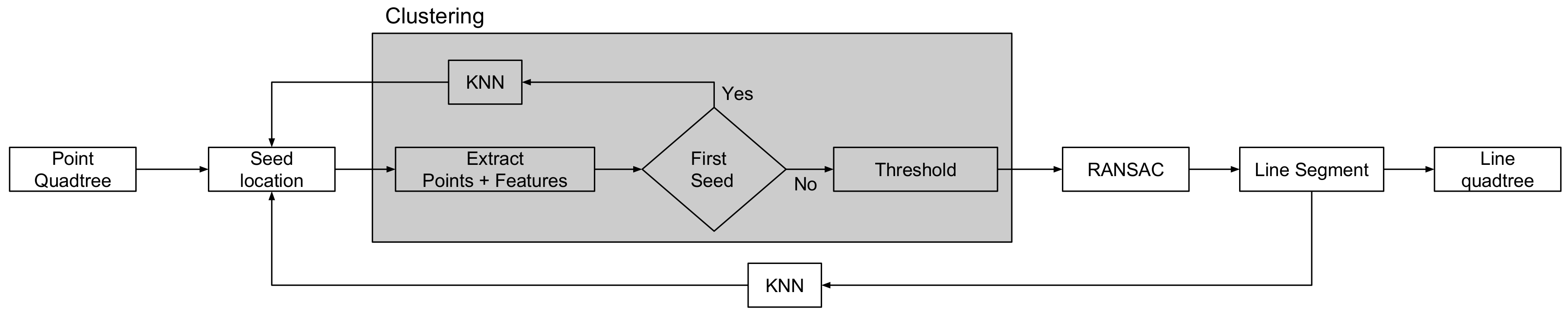
4.1. Line Segment Extraction
- The first step in the clustering process is the extraction of all environment points at location by recursively visiting the environment model. Furthermore, the principal components will be computed for these points. In the case of the first seed location, the address of the nearest neighbor node will be added to the list of seed locations by applying the KNN algorithm.
- The clustering process defines if both datasets are part of the same cluster or not. This process uses a predefined threshold . In the case of the simplified example, this threshold was configured to .
- The region growing process selects the next nearest neighbor node in order to cluster the new node. This process keeps searching for nodes that contain environmental points until all nodes are visited. Finally, line segments have to be created based on the clusters that were found. To do this, two approaches are possible:
- (a)
- a RANdom SAmple Consensus (RANSAC) algorithm, which automatically excludes outliers, so that the optimal line segment can be found regarding the points of each cluster. One of the advantages of this approach is that an optimal line segment will be found according to the given points. When the number of points is low, it is hard to get an optimal line segment since RANSAC needs to sample random samples of different point pairs.
- (b)
- connecting the centroids of the set of points of each cluster. The main disadvantage of this approach is that the number of clusters has to be large so that it performs an accurate segmentation.
4.2. Device Configuration
- Transmitter location ,
- Transmitter power (dBm),
- Transmitter antenna gain (dB),
- Radiation pattern (monopole, dipole),
- Number of rays,
- Maximum level of the reflection tree,
- Receiver location ,
- Receiver antenna gain (dB),
- Maximum level of the environment model,
- Environment model.
4.3. Ray Calibration
- A depth-first search algorithm that recursively traces the Quadtree data structure until location fits within the range of the node.
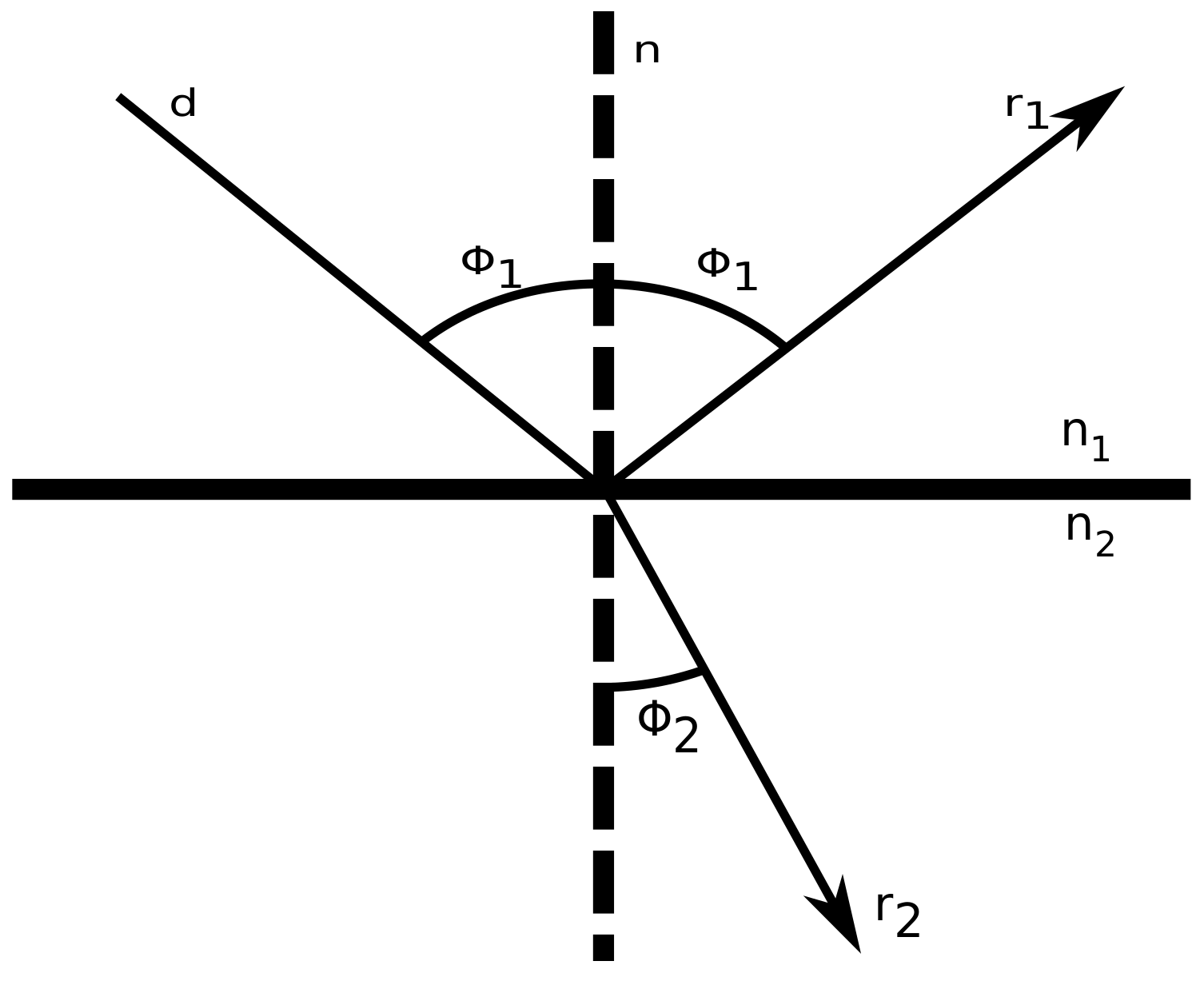
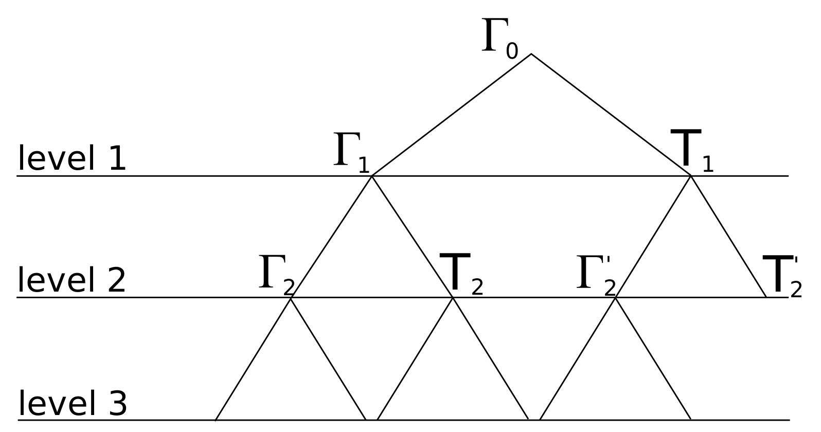
- An algorithm that keeps track of the visited cell list and ensures that the recursion level of the reflection is smaller then the pre-configured level. Because of the fact that each ray is inserted into the environment model by splitting each ray in small line segments with a permittivity of 1, an intersection point between an environment line segment and a ray segment can be computed with traditional mathematics. This intersection only occurs when the Quadtree node contains an environment object. Since each reflection and transmission is traced in a recursive fashion, the following Figure 8 illustrates the recursion order that each ray undergoes. At the first intersection , a reflection and transmission occurs. Second, because of the depth first implementation, is the next reflection intersection. Since appears at level 2 and the pre-configured level is equal to 3 this ray will be traced in the direction of the reflection angle and will stop at the following intersection. Subsequently, the returning recursion will trace in the direction of the refraction angle. Third, as a result of the recursive implementation, the intersection at refraction is found and traced. Finally, the other reflections and refractions are found and traced in a similar approach.
- Detecting if the ray is part of the current Quadtree node. This process includes the estimation where the ray segment denoted by and is crossing the axis- aligned bounding box defined by and . Since each ray segment can be expressed as , where m denotes the slope and b the location where the segment crosses the y-axis. On the other hand, an edge of an axis-aligned bounding is always parallel with one of the coordinate axis. This means that expresses a line that is parallel with the x-axis. In order to check if the ray crosses this Quadtree node, and needs to be incorporated so that all line equation that refers to the edges of the bounding box are crossing with the ray segment or not. In case when a ray is crossing any ray segments, the algorithm increase the ray segment so that is located in the next Quadtree cell. This makes it possible for the next recursion to locate the next Quadtree node that is part of the ray.
- Since the traversal algorithm traverses a ray in a Quadtree data structure according to a depth first search algorithm to localize each node, a tail recursion is applied that keeps the ray traversal algorithm running until the end of the ray is reached or the outer boundaries of the environment model are reached.
4.4. Electrical Field Computation
4.5. Applications
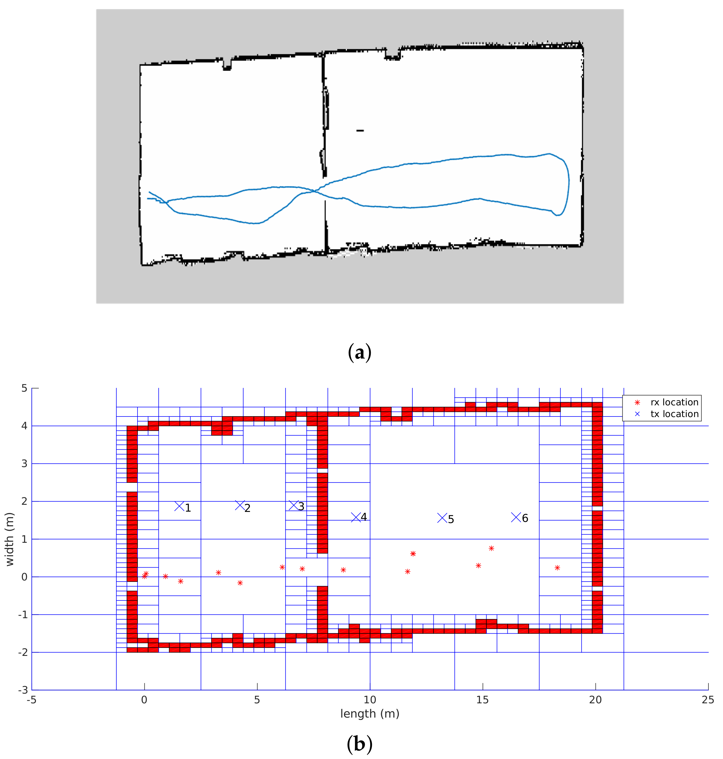
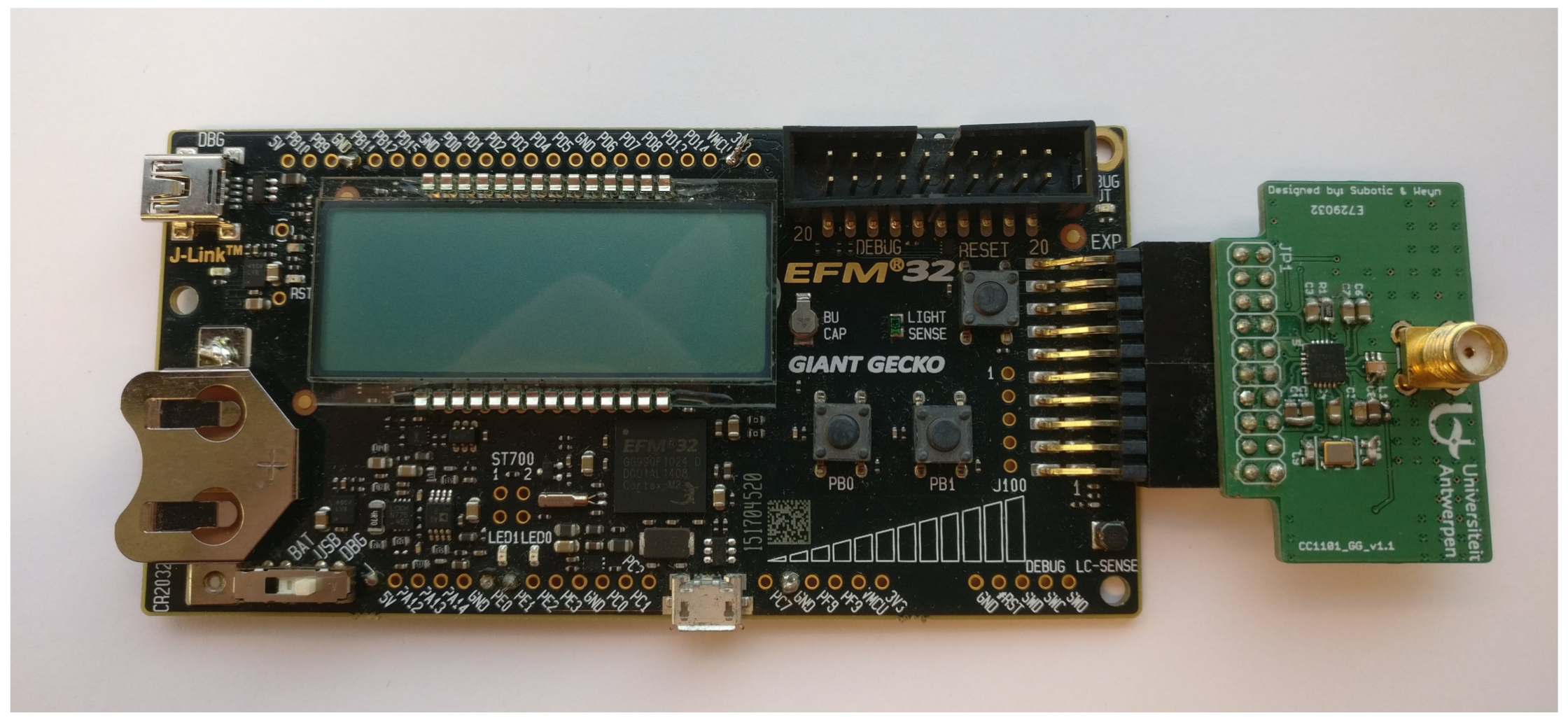
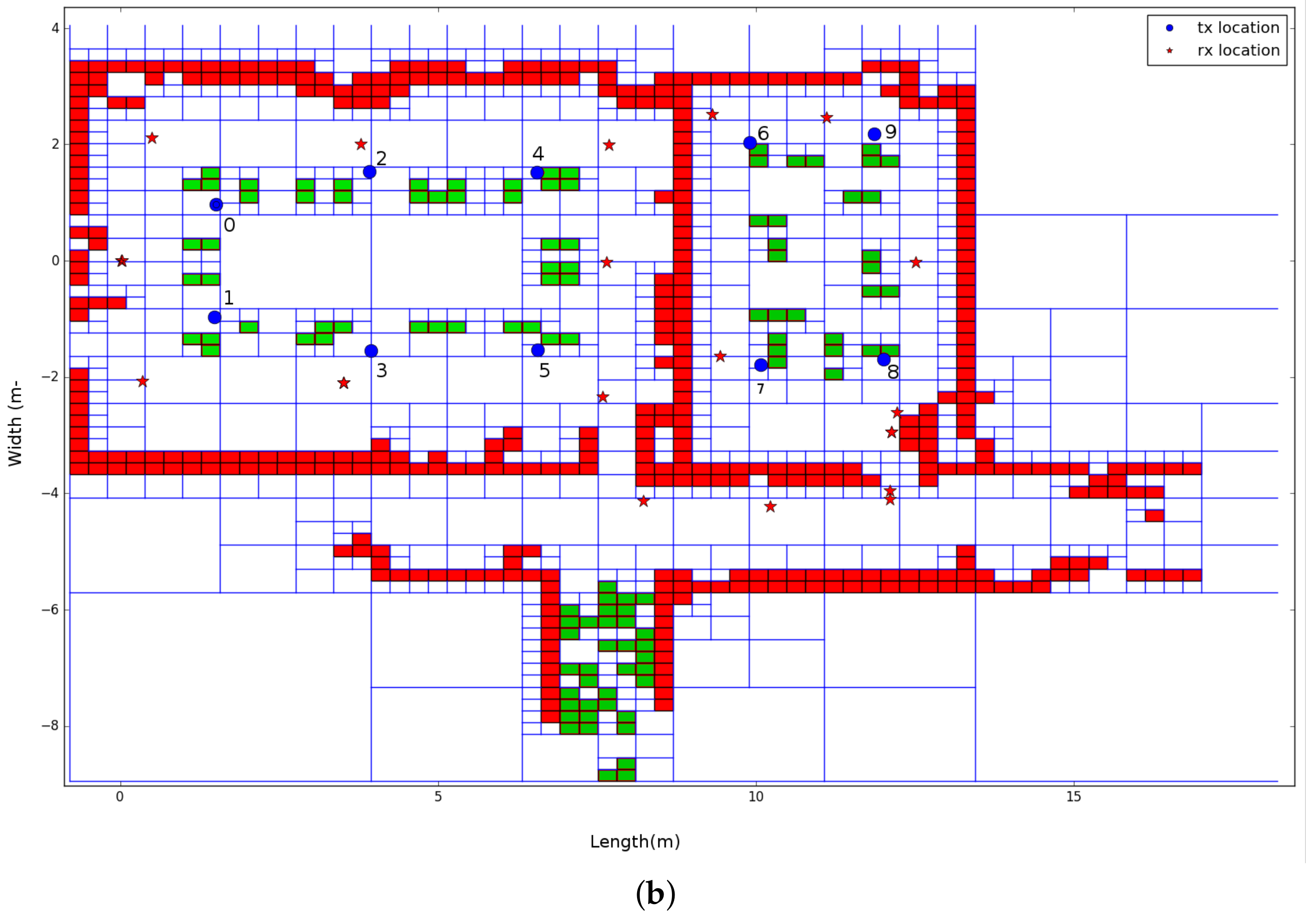
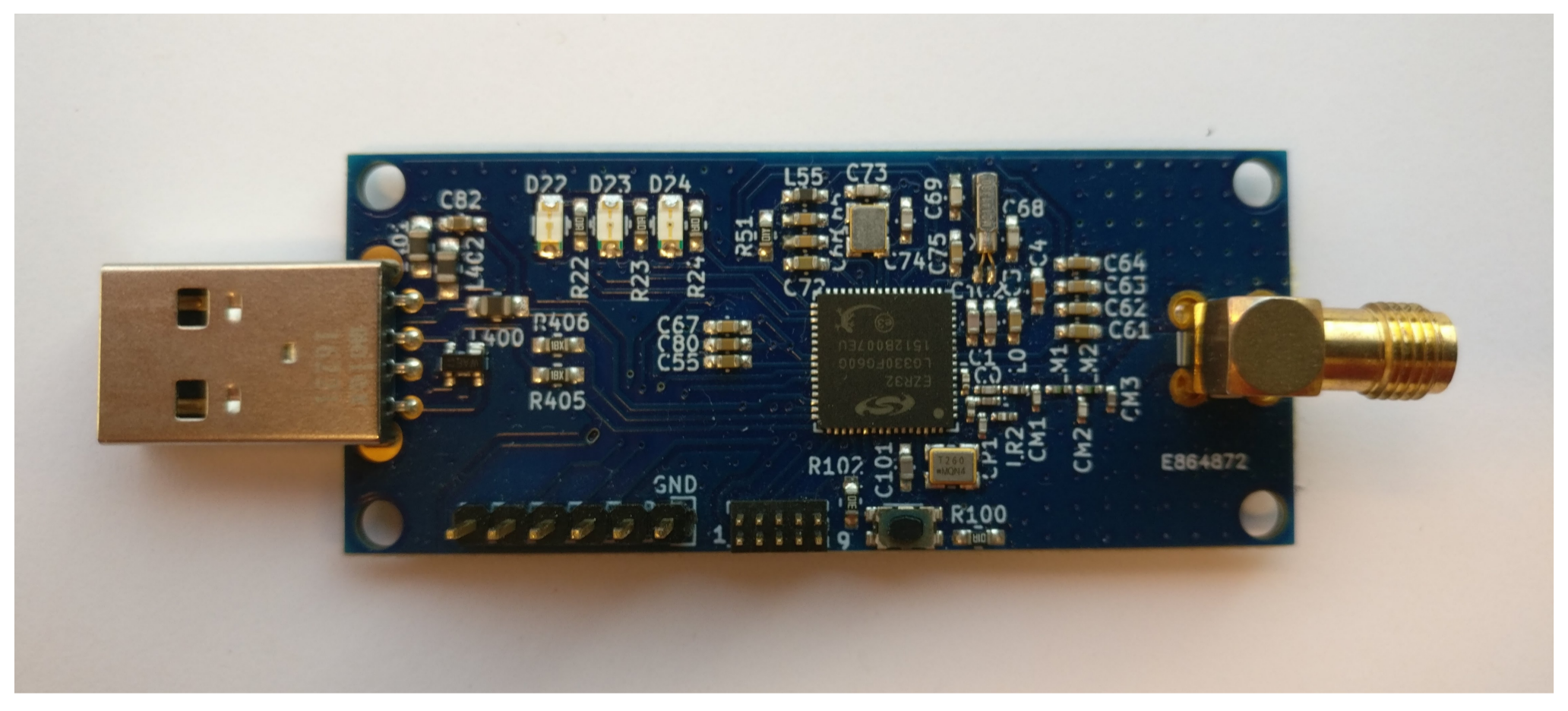
5. Materials
5.1. Validation Model
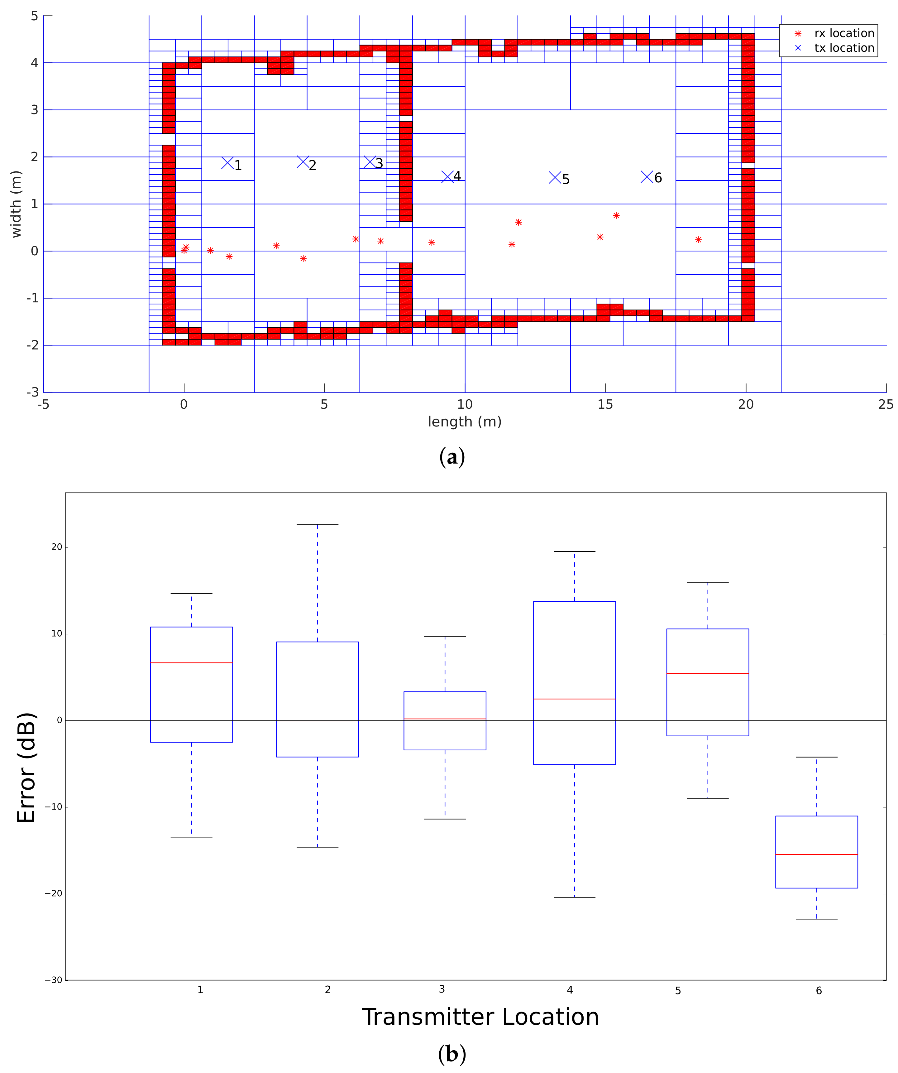
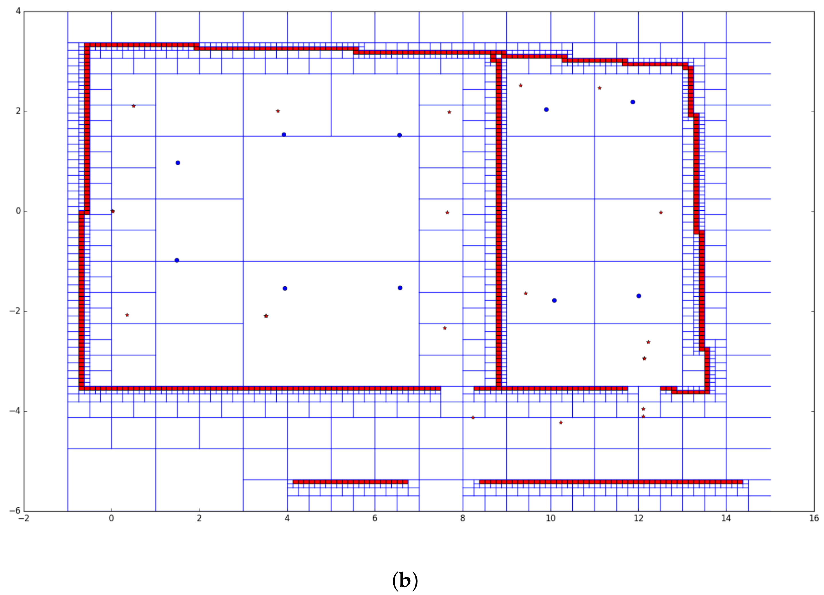
5.2. Test Environments
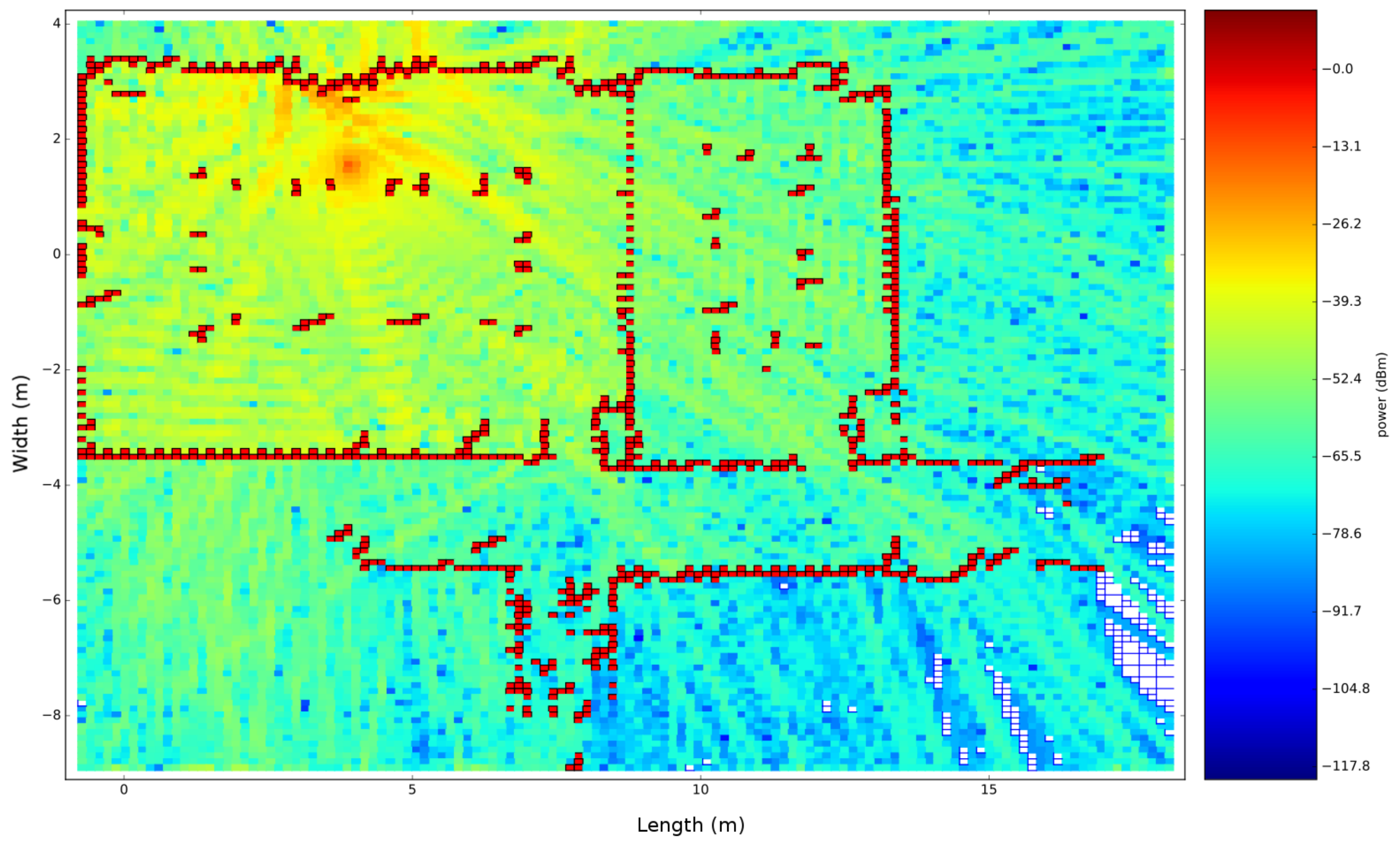
6. Results and Discussion
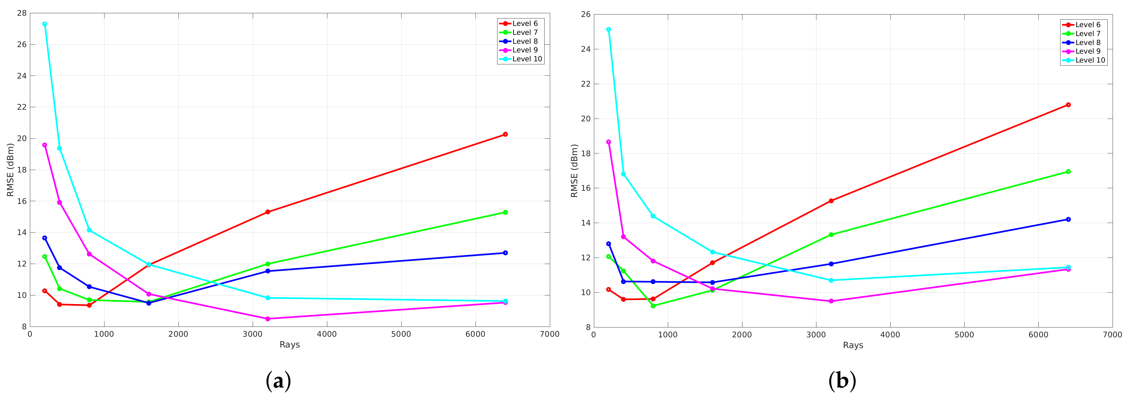
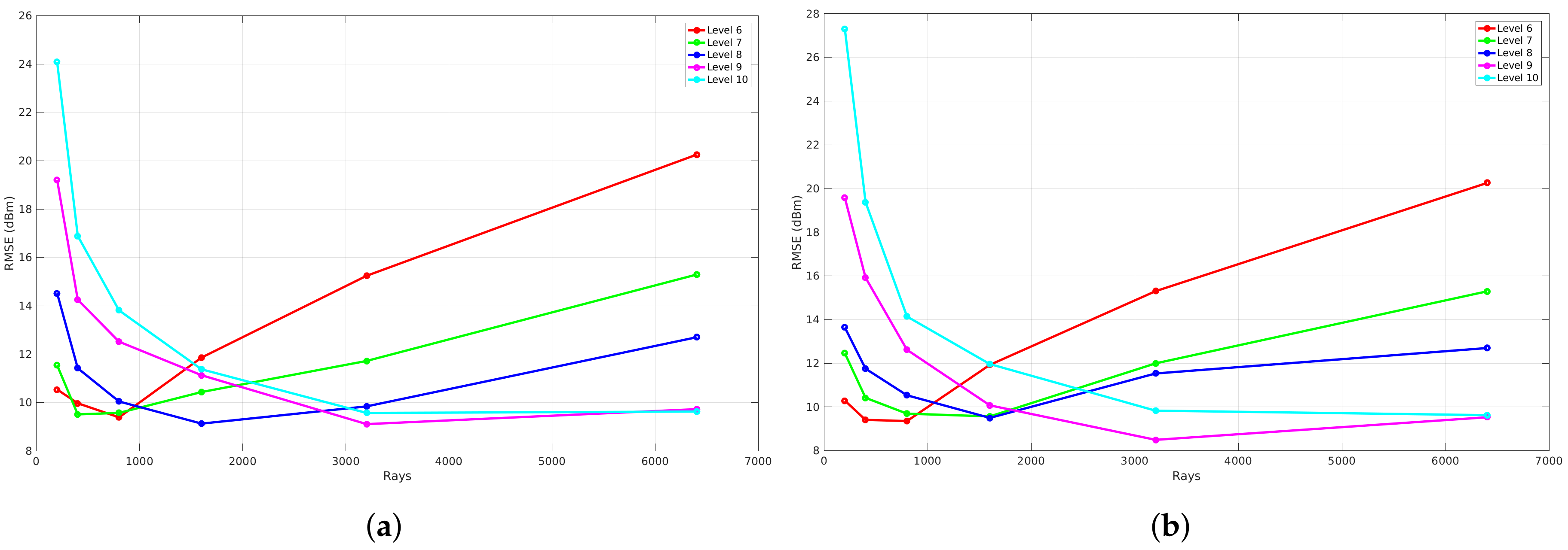
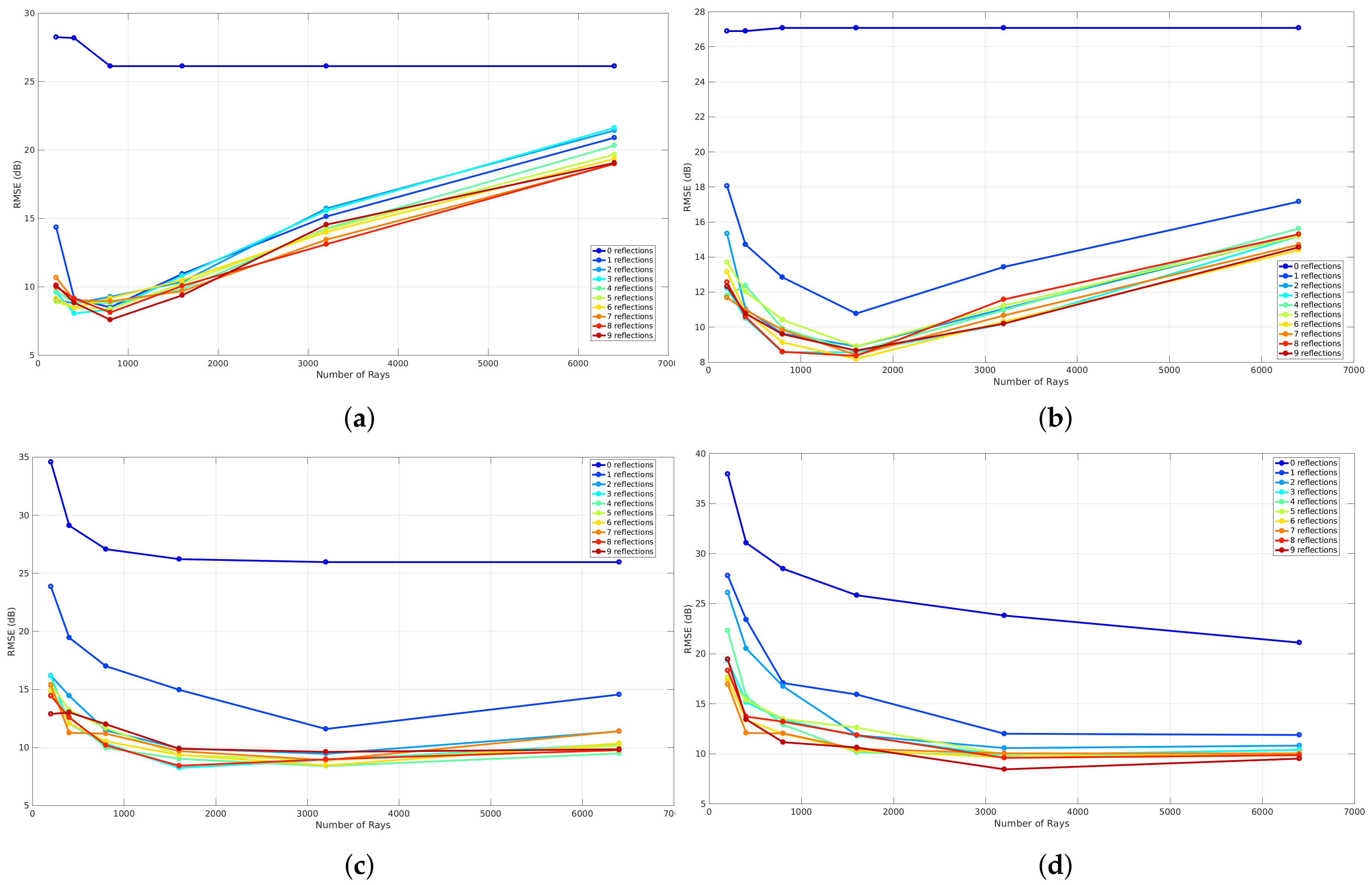
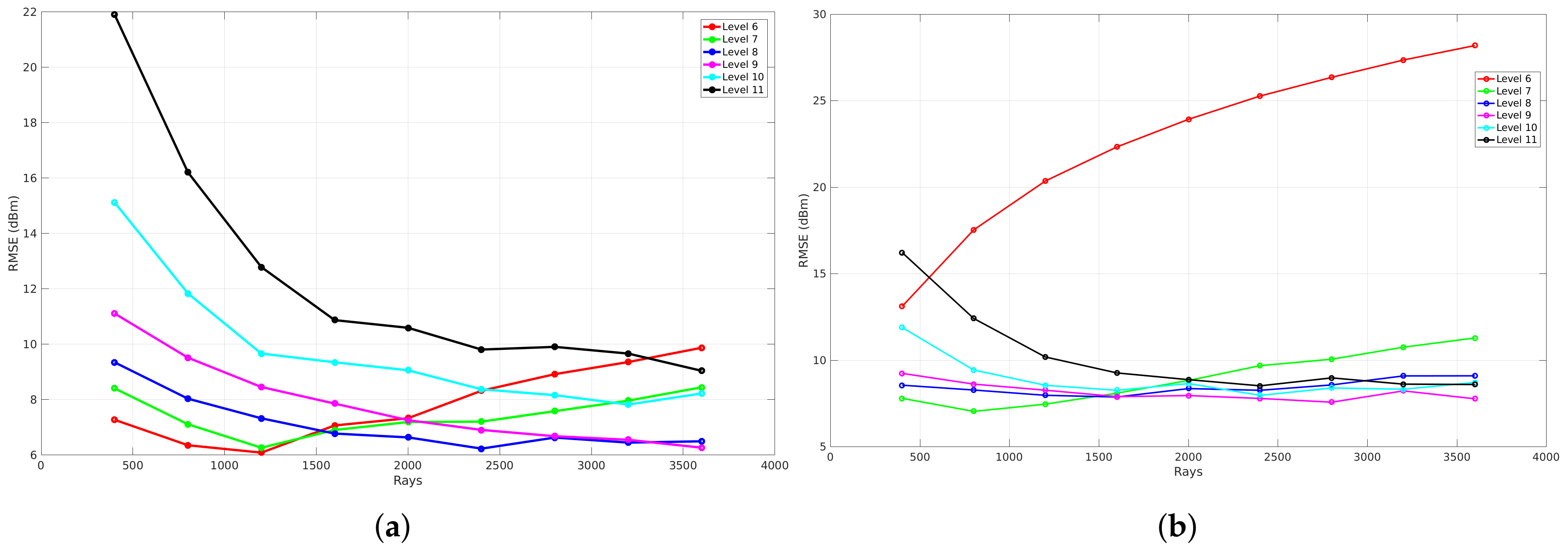
- By analyzing the correlation between the number of rays, the resolution of the environment, and a specific level of the reflection tree, the best global accuracy in terms of RMSE of all individual links is evaluated.
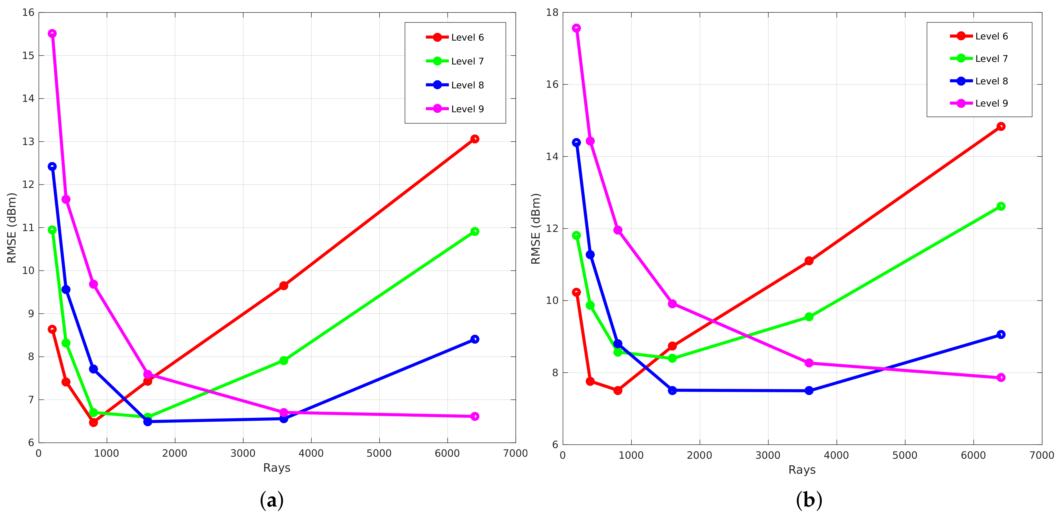
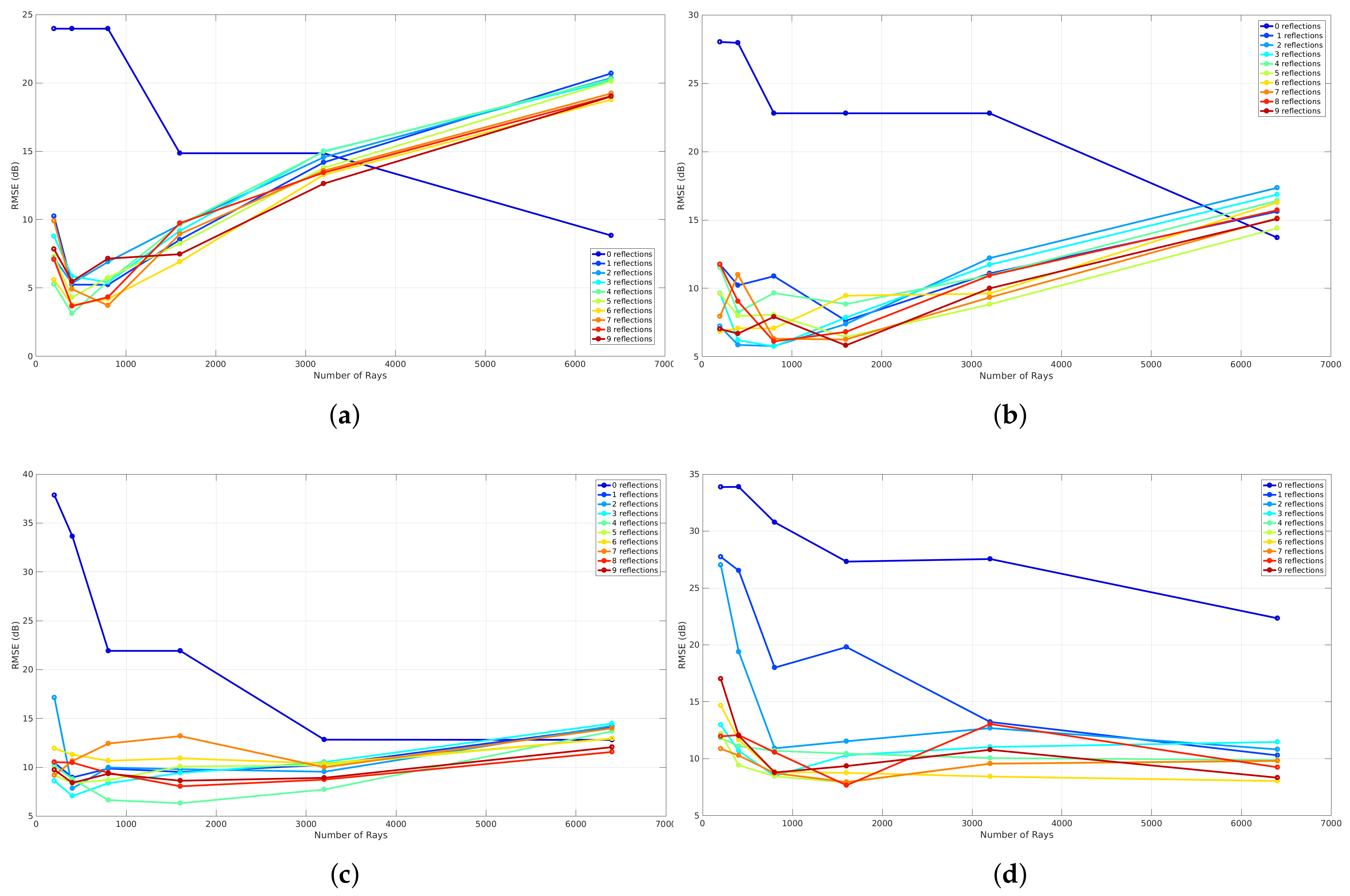
- The influence of the reflection tree level or changes in small scale fading is analyzed by simulating a different set of rays related to the RMSE according to different resolution levels of the environment.
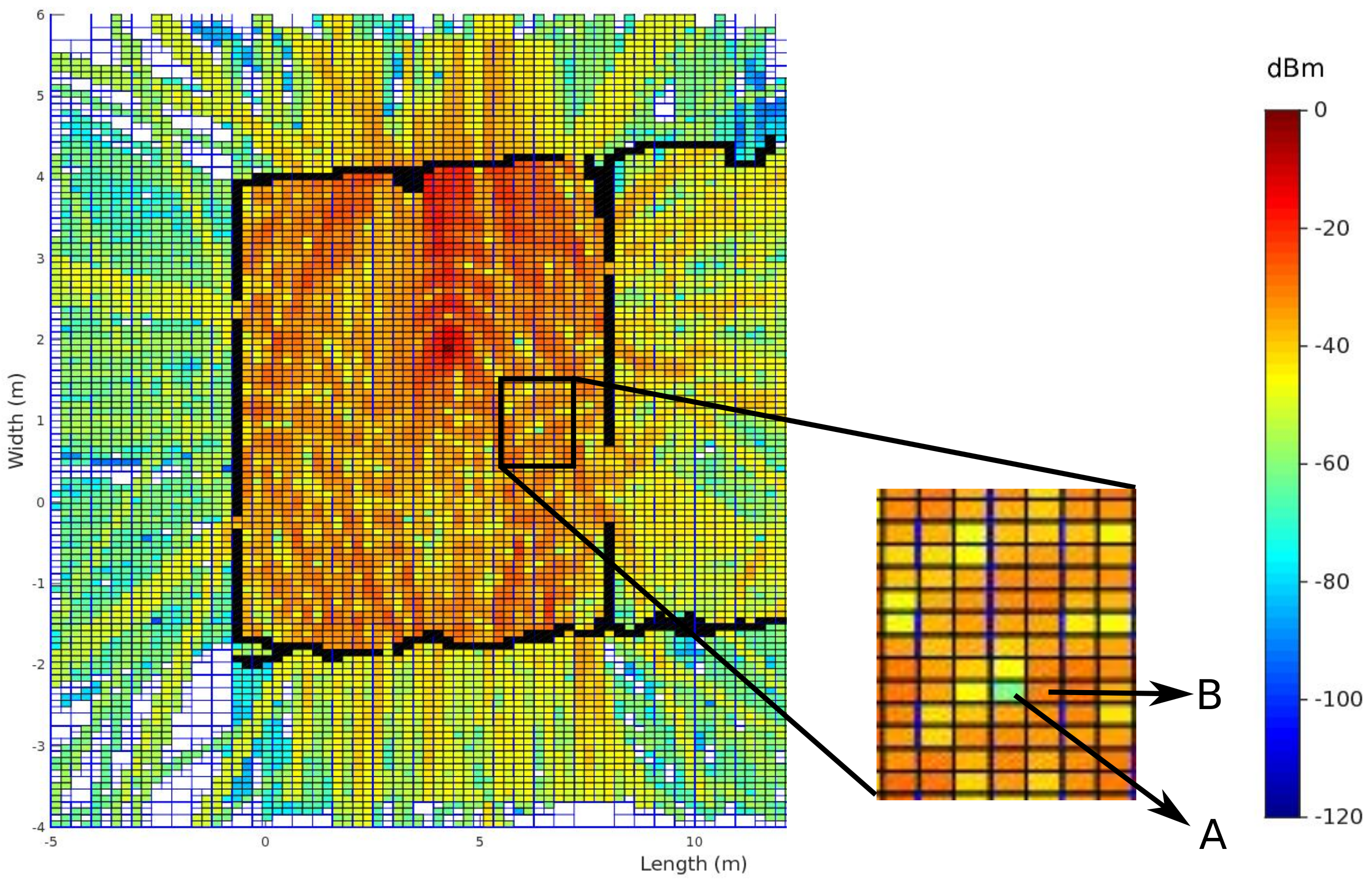
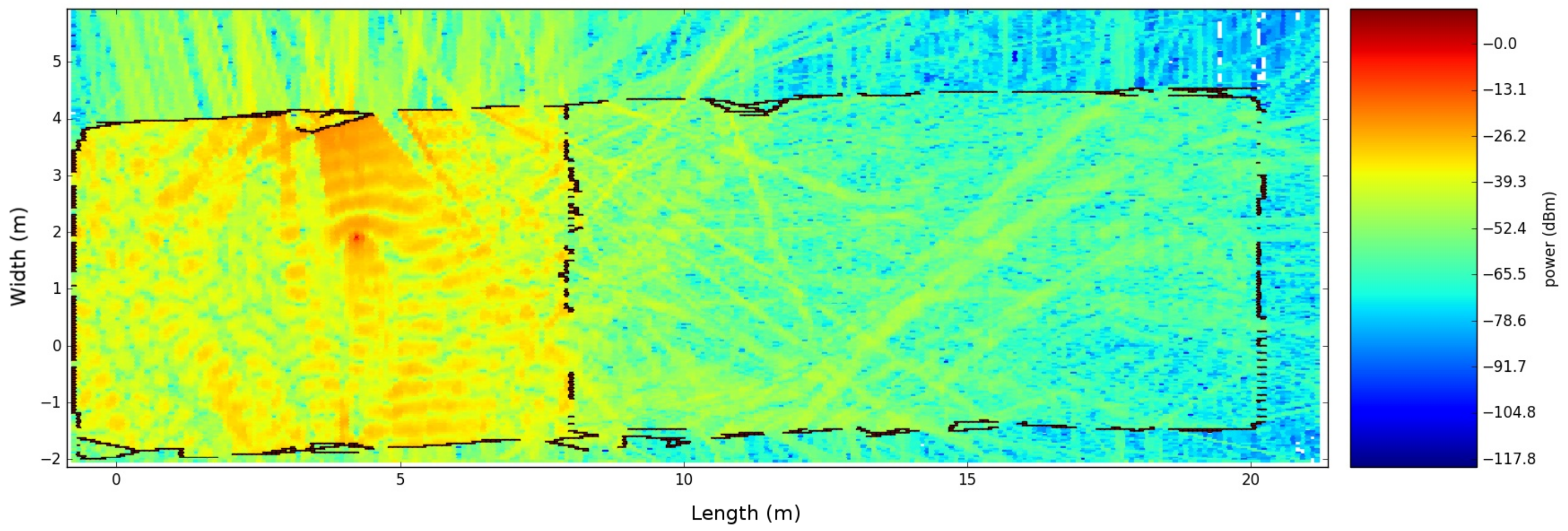
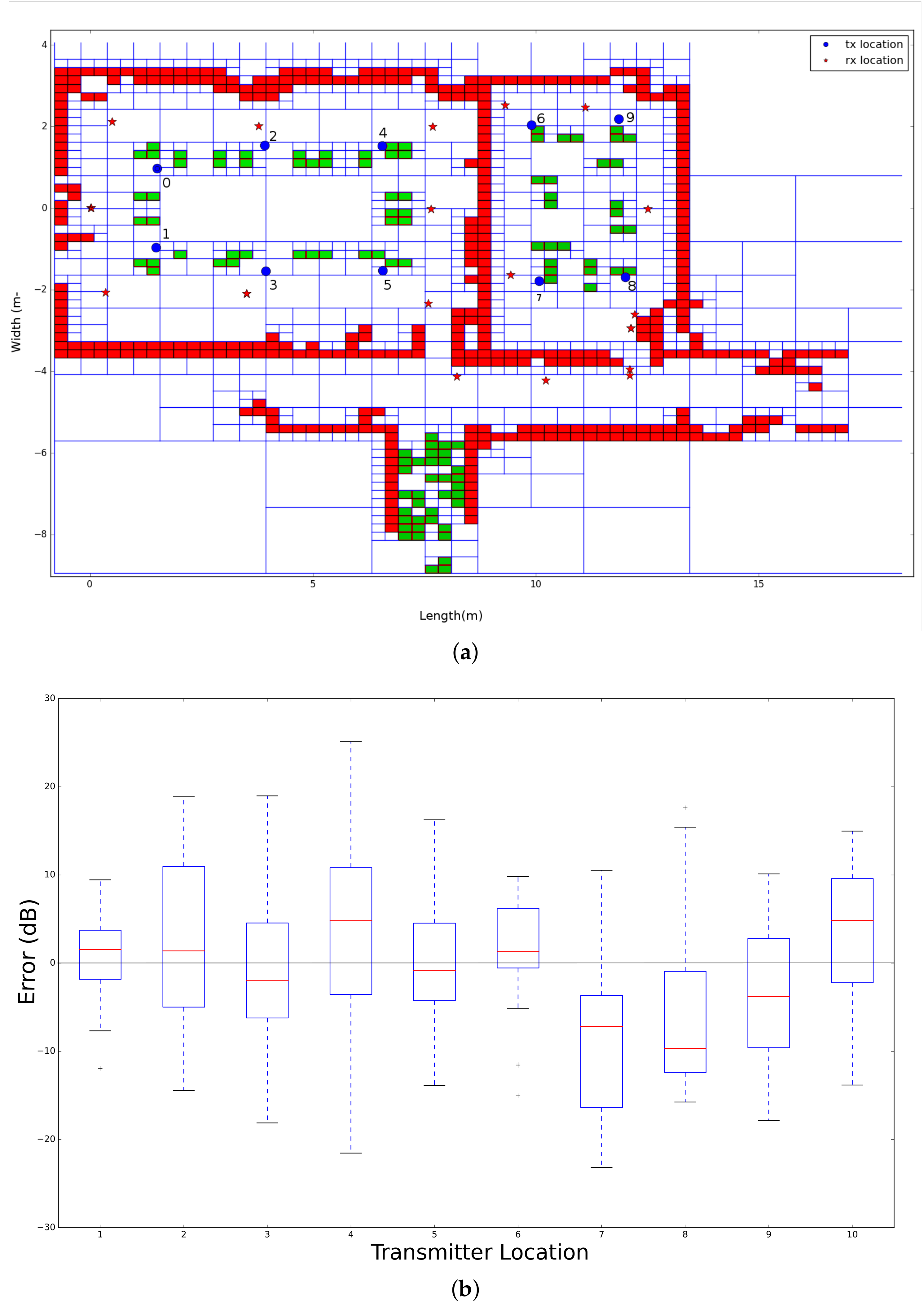
- The accuracy of all transmitters is evaluated by analyzing the differences between the simulated signal strength and the measured signal strength that was measured during one minute at the different receiver locations in terms of the ME, the MAE, the RMSE, and the precision.
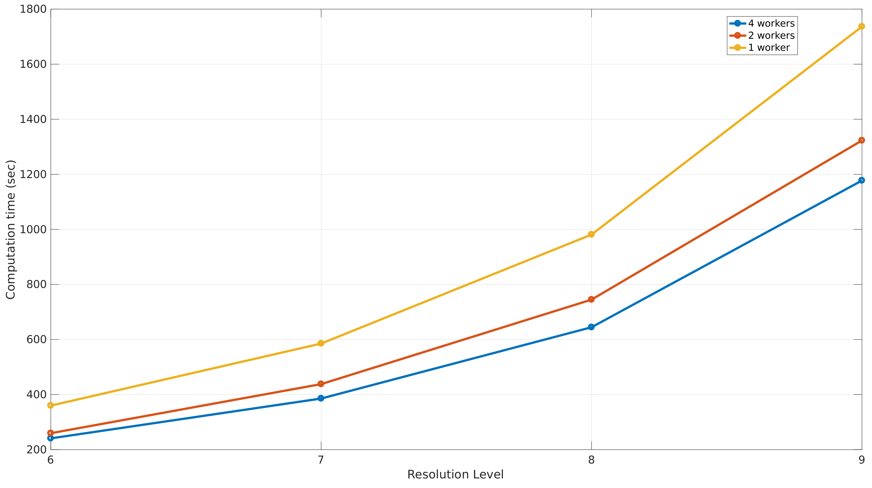
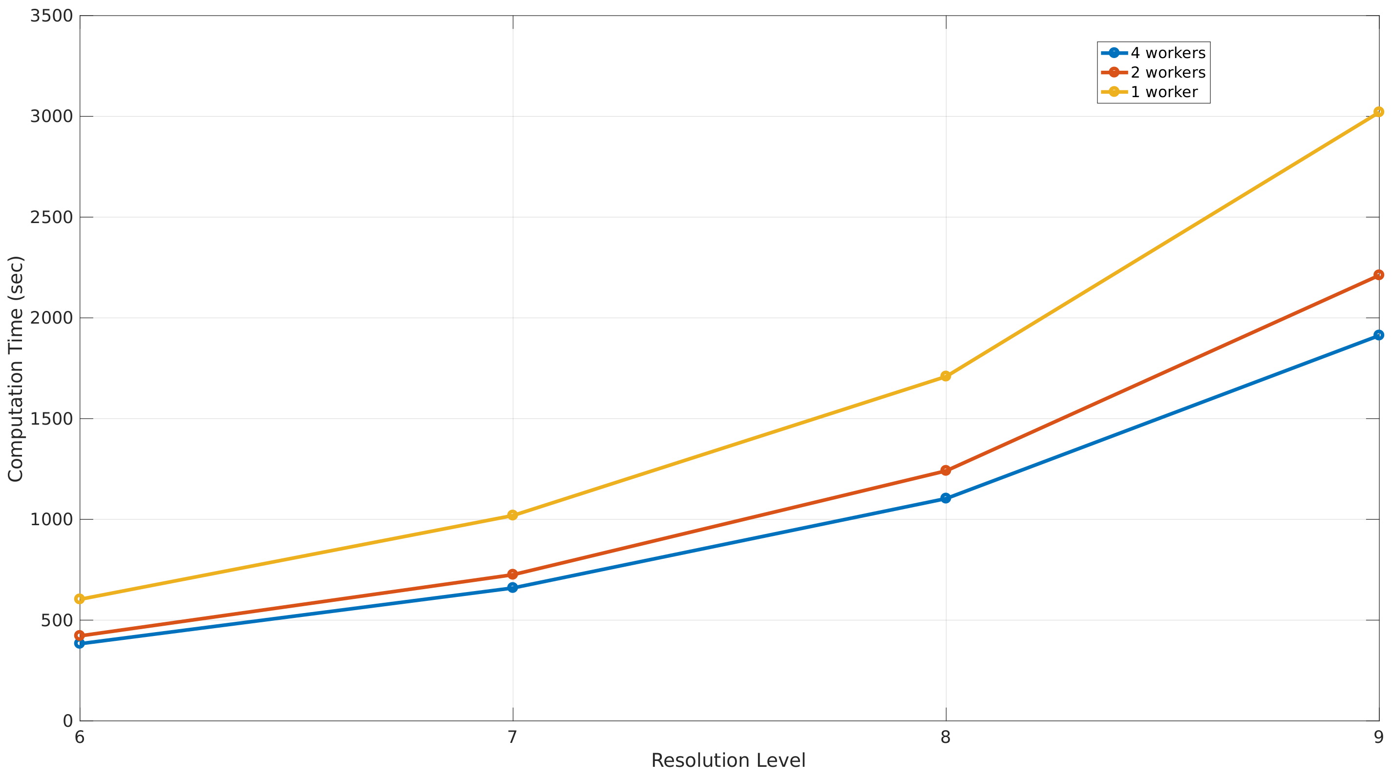
- The performance of the propagation loss model is analyzed related to the number processing units and the resolution of the environment. Furthermore, this analysis takes the optimal level of the reflection tree and the optimal number of rays as input.
6.1. Office Environment 1
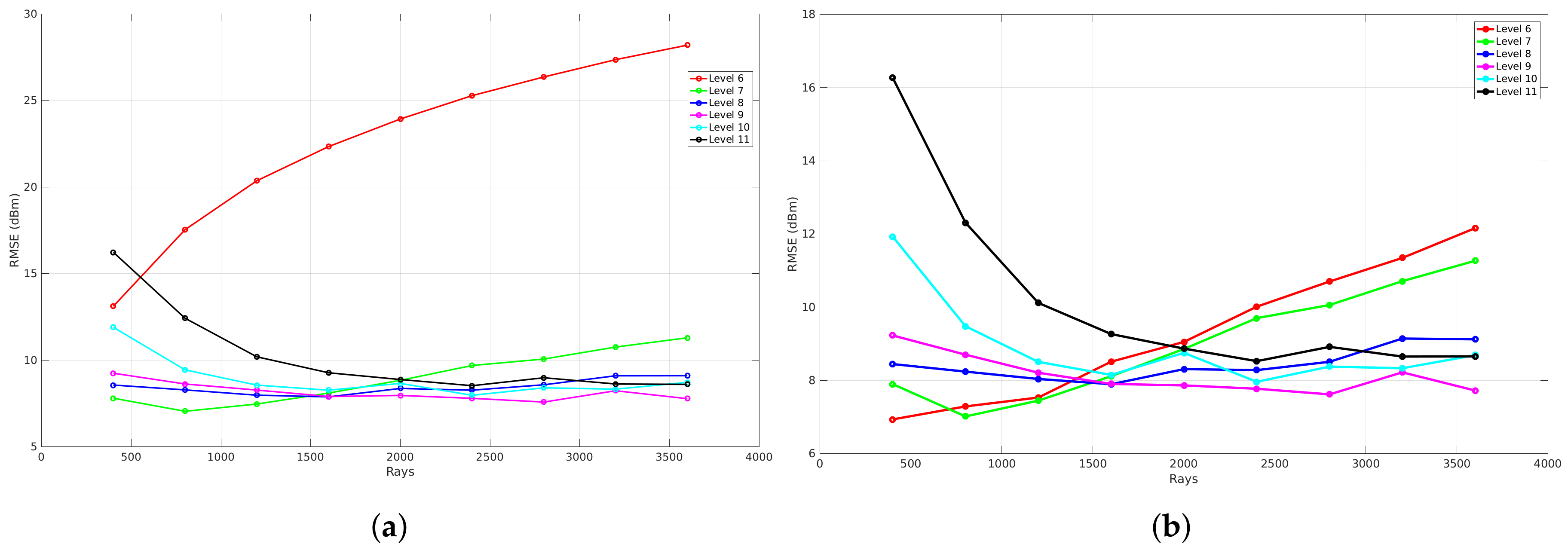
6.1.1. Resolution
6.1.2. Reflections
6.1.3. Validation
6.1.4. Performance
6.2. Office Environment 2
6.2.1. Resolution
6.2.2. Reflections
6.2.3. Validation
6.2.4. Performance
7. Conclusions
Author Contributions
Funding
Conflicts of Interest
References
- Iskander, M.F.; Yun, Z. Propagation prediction models for wireless communication systems. IEEE Trans. Microw. Theory Tech. 2002, 50, 662–673. [Google Scholar] [CrossRef]
- Almers, P.; Bonek, E.; Burr, A.; Czink, N.; Debbah, M.; Degli-Esposti, V.; Hofstetter, H.; Kyösti, P.; Laurenson, D.; Matz, G.; et al. Survey of Channel and Radio Propagation Models for Wireless MIMO Systems. EURASIP J. Wirel. Commun. Netw. 2007, 2007, 019070. [Google Scholar] [CrossRef]
- Forooshani, A.E.; Bashir, S.; Michelson, D.G.; Noghanian, S. A survey of wireless communications and propagation modeling in underground mines. IEEE Commun. Surv. Tutor. 2013, 15, 1524–1545. [Google Scholar] [CrossRef]
- Azpilicueta, L.; Rawat, M.; Rawat, K.; Ghannouchi, F.M.; Falcone, F. A Ray Launching-Neural Network Approach for Radio Wave Propagation Analysis in Complex Indoor Environments. IEEE Trans. Antennas Propag. 2014, 62, 2777–2786. [Google Scholar] [CrossRef]
- Subrt, L.; Pechac, P. Advanced 3D indoor propagation model: calibration and implementation. EURASIP J. Wirel. Commun. Netw. 2011, 2011, 180. [Google Scholar] [CrossRef]
- Yun, Z.; Iskander, M.F. Ray Tracing for Radio Propagation Modeling: Principles and Applications. IEEE Access 2015, 3, 1089–1100. [Google Scholar] [CrossRef]
- Bellekens, B.; Penne, R.; Weyn, M. Validation of an indoor ray launching RF propagation model. In Proceedings of the 2016 IEEE-APS Topical Conference on Antennas and Propagation in Wireless Communications (APWC), Cairns, QLD, Australia, 19–23 September 2016; pp. 74–77. [Google Scholar]
- Letourneux, F.; Guivarch, S.; Lostanlen, Y. Propagation models for Heterogeneous Networks. In Proceedings of the 2013 7th European Conference on Antennas and Propagation (EuCAP), Gothenburg, Sweden, 8–12 April 2013; pp. 3993–3997. [Google Scholar]
- Ayadi, M.; Torjemen, N.; Tabbane, S. Two-Dimensional Deterministic Propagation Models Approach and Comparison With Calibrated Empirical Models. IEEE Trans. Wirel. Commun. 2015, 14, 5714–5722. [Google Scholar] [CrossRef]
- Tam, W.; Tran, V. Propagation modelling for indoor wireless communication. Electron. Commun. Eng. J. 1995, 7, 221–228. [Google Scholar] [CrossRef]
- Dissanayake, M.; Newman, P.; Clark, S.; Durrant-Whyte, H.; Csorba, M. A solution to the simultaneous localization and map building (SLAM) problem. IEEE Trans. Robot. Autom. 2001, 17, 229–241. [Google Scholar] [CrossRef]
- Grisetti, G.; Stachniss, C.; Burgard, W. Improved Techniques for Grid Mapping With Rao–Blackwellized Particle Filters. IEEE Trans. Robot. 2007, 23, 34–46. [Google Scholar] [CrossRef]
- Plets, D.; Joseph, W.; Vanhecke, K.; Tanghe, E.; Martens, L. Coverage prediction and optimization algorithms for indoor environments. EURASIP J. Wirel. Commun. Netw. 2012, 2012, 123. [Google Scholar] [CrossRef]
- Torres, R.P. CINDOOR: Computer tool for planning and design of wireless systems in enclosed spaces. Microw. Eng. Eur. 1997, 41, 11–22. [Google Scholar]
- Weyn, M.; Ergeerts, G.; Berkvens, R.; Wojciechowski, B.; Tabakov, Y. DASH7 alliance protocol 10: Low-power, mid-range sensor and actuator communication. In Proceedings of the 2015 IEEE Conference on Standards for Communications and Networking (CSCN), Tokyo, Japan, 28–30 October 2015; pp. 54–59. [Google Scholar]
- Sato, R.; Sato, H.; Shirai, H. A SBR algorithm for simple indoor propagation estimation. In Proceedings of the 2005 IEEE/ACES International Conference on Wireless Communications and Applied Computational Electromagnetics, Honolulu, HI, USA, 3–7 April 2005; pp. 812–815. [Google Scholar]
- Imai, T. A survey of efficient ray-tracing techniques for mobile radio propagation analysis. IEICE Trans. Commun. 2017, 100, 666–679. [Google Scholar] [CrossRef]
- Nagy, L. FDTD and Ray and Optical Methods and for Indoor and Wave and Propagation Modeling. Available online: https://pdfs.semanticscholar.org/4652/d81b8341dcea61eb86f7480bbb342fd0392c.pdf (accessed on 31 May 2018).
- Klepal, M. Novel Approach to Indoor Electromagnetic Wave Propagation Modelling. Ph.D. Thesis, Czech Technical University in Prague, Prague, Czech Republic, 2003. [Google Scholar]
- Lai, Z.; Bessis, N.; De La Roche, G.; Zhang, J.; Clapworthy, G.; Kuonen, P.; Zhou, D. Intelligent ray launching algorithm for indoor scenarios. Radioengineering 2011, 20, 398. [Google Scholar]
- Durrant-Whyte, H.; Bailey, T. Simultaneous localization and mapping: Part I. IEEE Robot. Autom. Mag. 2006, 13, 99–110. [Google Scholar] [CrossRef]
- Dissanayake, G. A computationally efficient solution to the simultaneous localisation and map building (SLAM) problem. In Proceedings of the IEEE International Conference on Robotics and Automation (ICRA ’00), San Francisco, CA, USA, 24–28 April 2000; Volume 2, pp. 1009–1014. [Google Scholar]
- Eliazar, A.; Parr, R. DP-SLAM: Fast, robust simultaneous localization and mapping without predetermined landmarks. IJCAI 2003, 3, 1135–1142. [Google Scholar]
- Gutmann, J.S.; Konolige, K. Incremental mapping of large cyclic environments. In Proceedings of the 1999 IEEE International Symposium on Computational Intelligence in Robotics and Automation, Monterey, CA, USA, 8–9 November 1999; pp. 318–325. [Google Scholar]
- Zachmann, G.; Langetepe, E. Geometric Data Structures for Computer Graphics. Synthesis 2003, 16, 1–54. [Google Scholar]
- Samet, H. The Quadtree and Related Hierarchical Data Structures. ACM Comput. Surv. 1984, 16, 187–260. [Google Scholar] [CrossRef]
- Moon, B.; Jagadish, H.V.; Faloutsos, C.; Saltz, J.H. Analysis of the Clustering of Hilbert Space-Filling Curve IEEE Trans. Knowl. Data Eng. 2001, 13, 124–141. [Google Scholar] [CrossRef]
- Richards, J.A. Radio Wave Propagation; Springer: Berlin/Heidelberg, Germany, 2008. [Google Scholar]


| Transmitter | (dB) | (dB) | (dB) | (dB) |
|---|---|---|---|---|
| 1 | 8.17 | 3.99 | 8.20 | 4.12 |
| 2 | 9.20 | 1.67 | 9.28 | 7.60 |
| 3 | 5.38 | −0.29 | 5.50 | 5.19 |
| 4 | 10.32 | 3.09 | 10.40 | 6.27 |
| 5 | 6.92 | 4.19 | 6.94 | 5.038 |
| 6 | 15.55 | −15.55 | 15.56 | 7.13 |
| (dB) | (dB) | (dB) | (dB) |
|---|---|---|---|
| 9.26 | −0.47 | 9.31 | 5.89 |
| Transmitter | (dB) | (dB) | (dB) | (dB) |
|---|---|---|---|---|
| 1 | 4.17 | 0.27 | 4.22 | 3.50 |
| 2 | 7.72 | 2.66 | 7.74 | 6.09 |
| 3 | 6.65 | −1.60 | 6.69 | 5.82 |
| 4 | 9.77 | 3.23 | 9.79 | 6.84 |
| 5 | 5.91 | 0.57 | 6.03 | 4.76 |
| 6 | 4.99 | 0.49 | 5.09 | 4.48 |
| 7 | 10.79 | −8.39 | 10.85 | 6.57 |
| 8 | 10.24 | −5.66 | 10.28 | 4.97 |
| 9 | 8.63 | −3.64 | 8.64 | 5.59 |
| 10 | 7.49 | 3.96 | 7.59 | 4.44 |
| (dB) | (dB) | (dB) | (dB) |
|---|---|---|---|
| 7.64 | −0.81 | 7.69 | 5.31 |
© 2018 by the authors. Licensee MDPI, Basel, Switzerland. This article is an open access article distributed under the terms and conditions of the Creative Commons Attribution (CC BY) license (http://creativecommons.org/licenses/by/4.0/).
Share and Cite
Bellekens, B.; Penne, R.; Weyn, M. Realistic Indoor Radio Propagation for Sub-GHz Communication. Sensors 2018, 18, 1788. https://doi.org/10.3390/s18061788
Bellekens B, Penne R, Weyn M. Realistic Indoor Radio Propagation for Sub-GHz Communication. Sensors. 2018; 18(6):1788. https://doi.org/10.3390/s18061788
Chicago/Turabian StyleBellekens, Ben, Rudi Penne, and Maarten Weyn. 2018. "Realistic Indoor Radio Propagation for Sub-GHz Communication" Sensors 18, no. 6: 1788. https://doi.org/10.3390/s18061788
APA StyleBellekens, B., Penne, R., & Weyn, M. (2018). Realistic Indoor Radio Propagation for Sub-GHz Communication. Sensors, 18(6), 1788. https://doi.org/10.3390/s18061788