Filter Selection for Optimizing the Spectral Sensitivity of Broadband Multispectral Cameras Based on Maximum Linear Independence


Abstract
1. Introduction
2. MLI Filter Selection Method
| Algorithm 1 Traditional MLI algorithm |
| Input S = 1; M;N; ; Procedure (1) Computer (2) Computer the norm set (3) IF S==1 (4) Find the objective filter (5) END IF (6) FOR S = 2:M (7) Delete from (8) Find (9) END FOR (10) Output The filter set selected by MLI with M spectral channels. |
3. Experimental Simulation
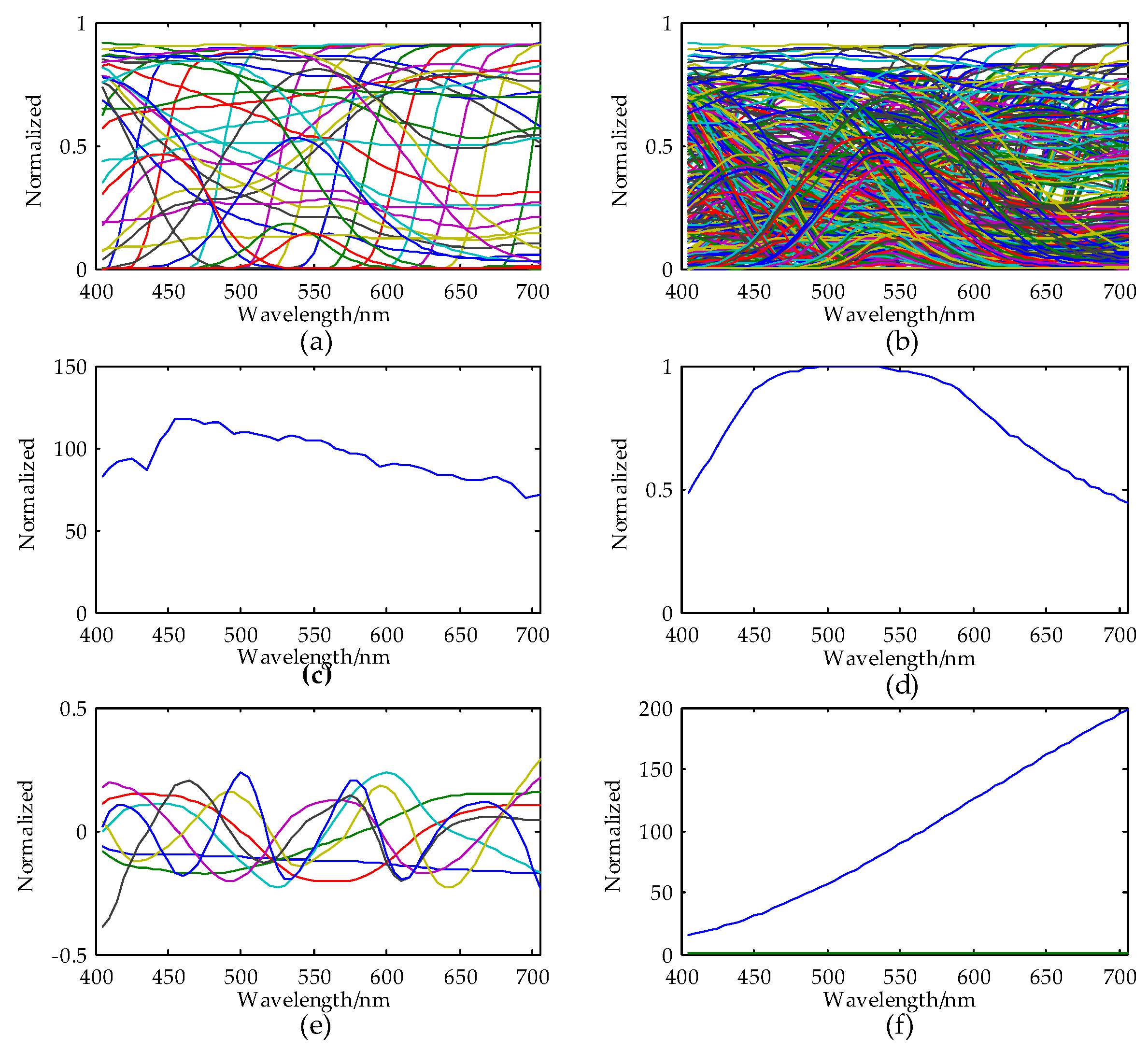
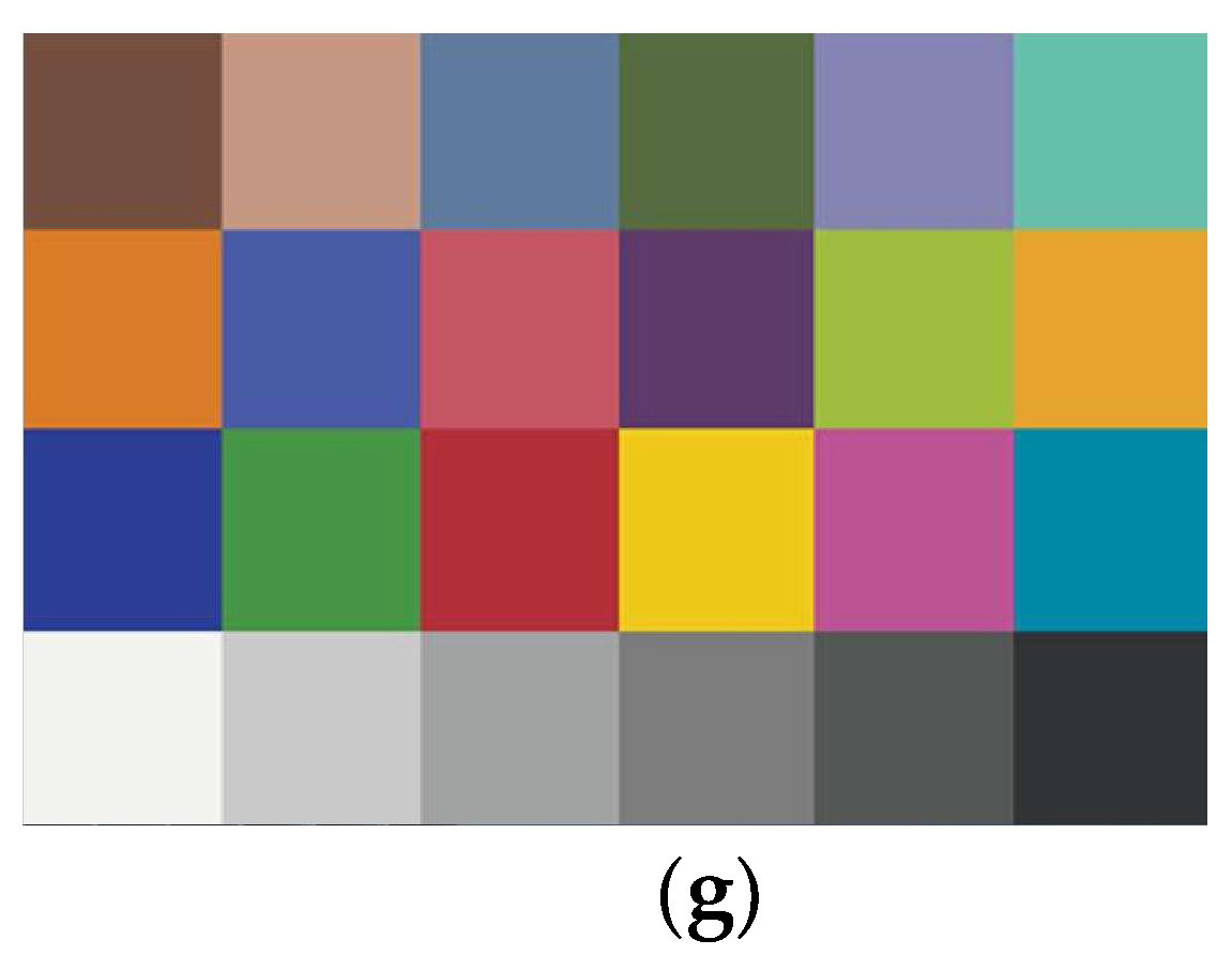
3.1. Datasets
3.2. Imaging Simulation and Evaluation
4. Data Process, Results and Analysis
4.1. Data Process Methods
4.1.1. Data Reduction
4.1.2. Data Sorting
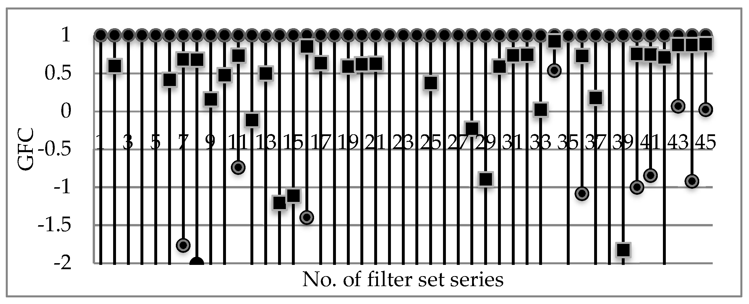
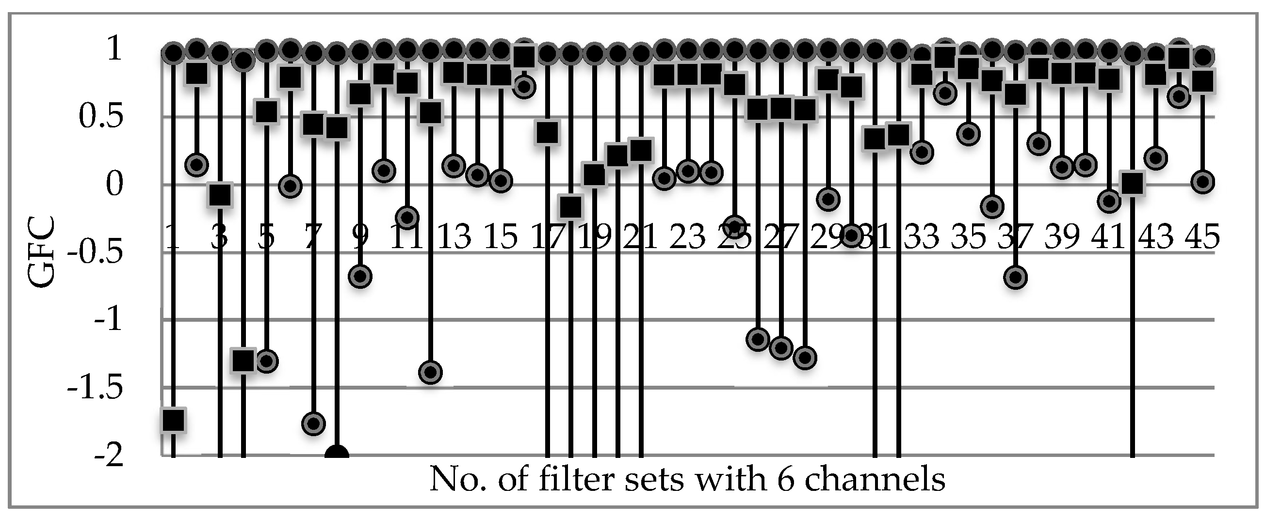
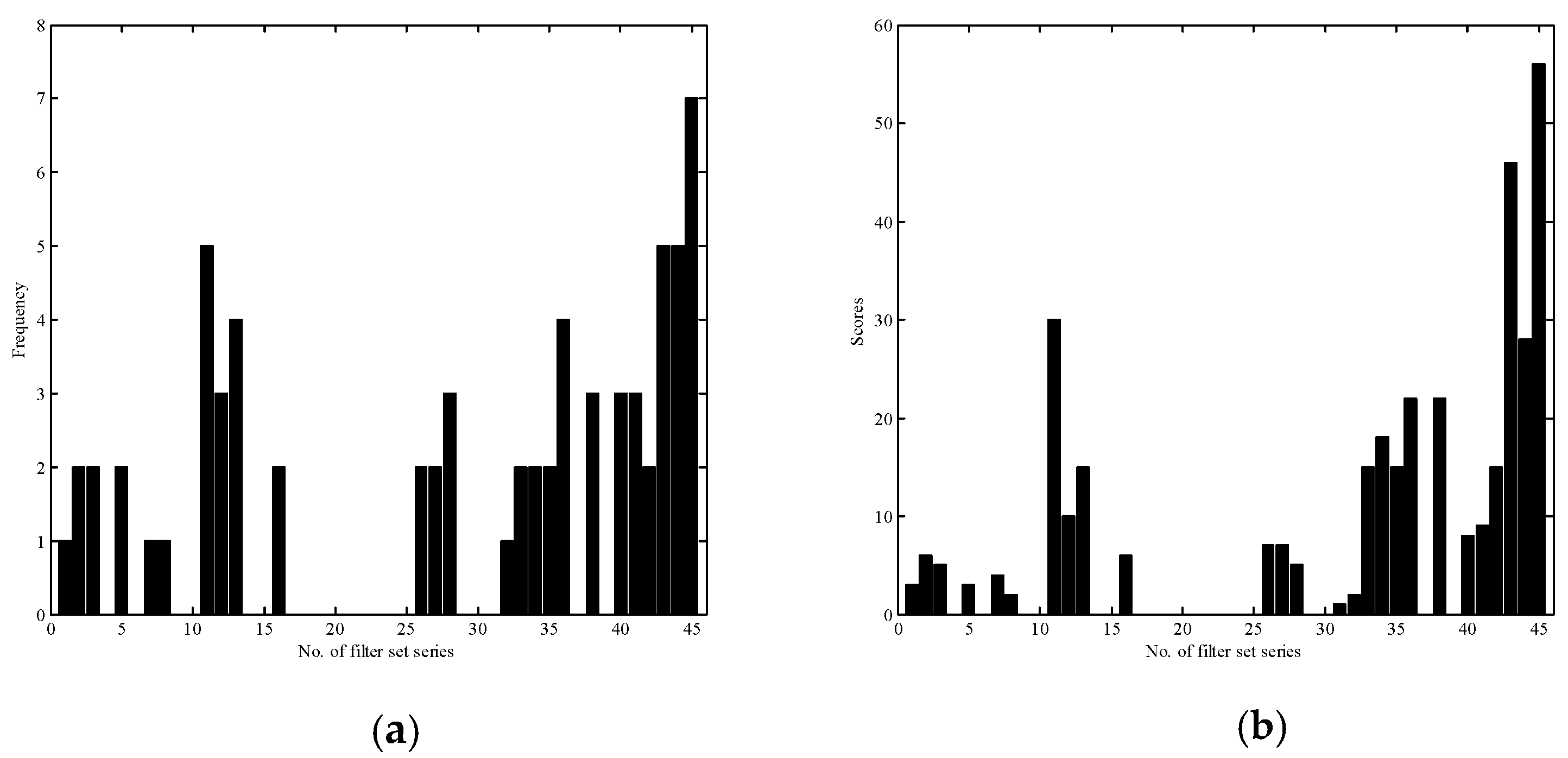
4.2. Results
4.2.1. Best-Performed Filter Sets
4.2.2. Comparison between the Best Filer Set and the Traditional Selection by MLI
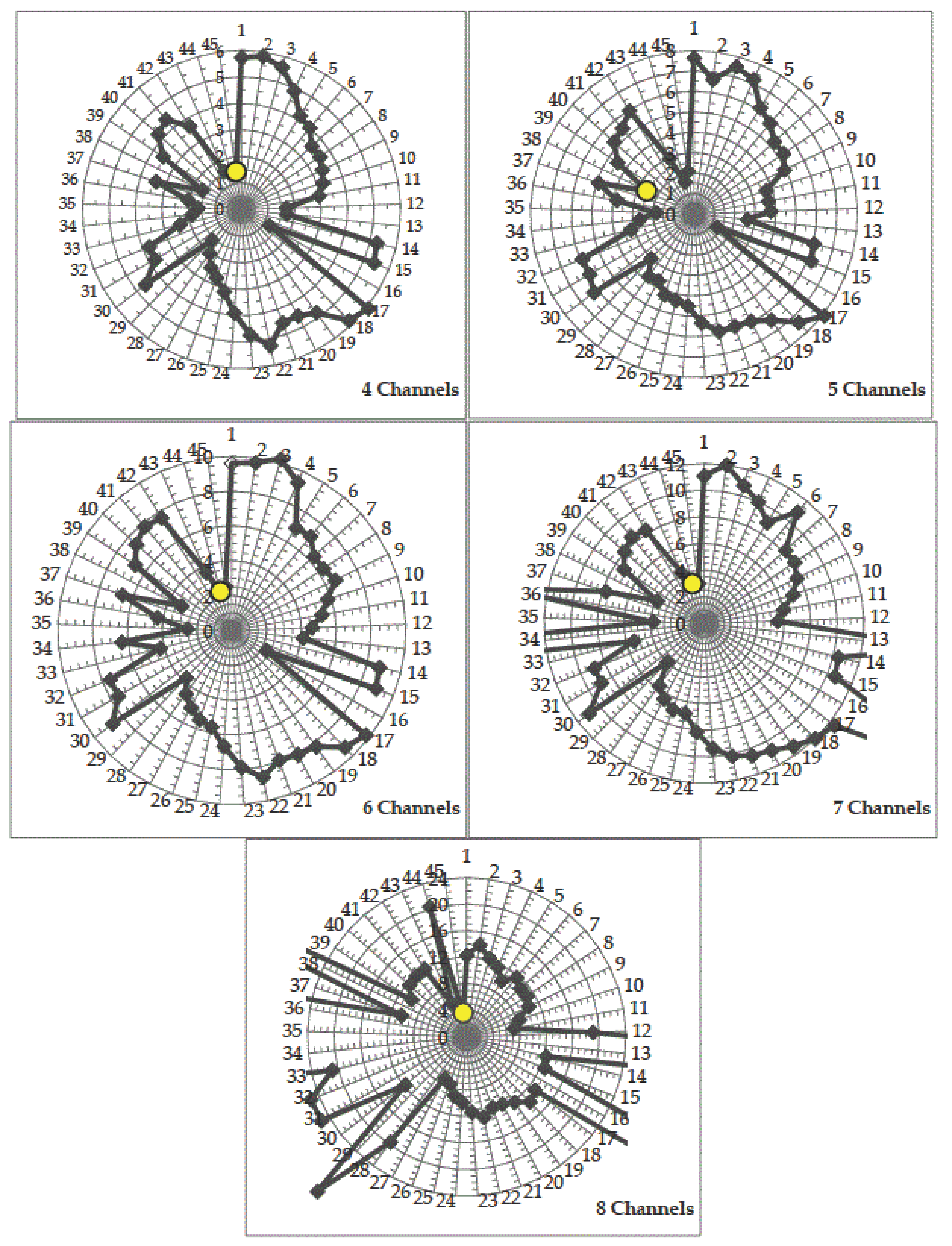
4.3. Characteristics of the Best-Performed Filter Sets
4.3.1. Condition Number
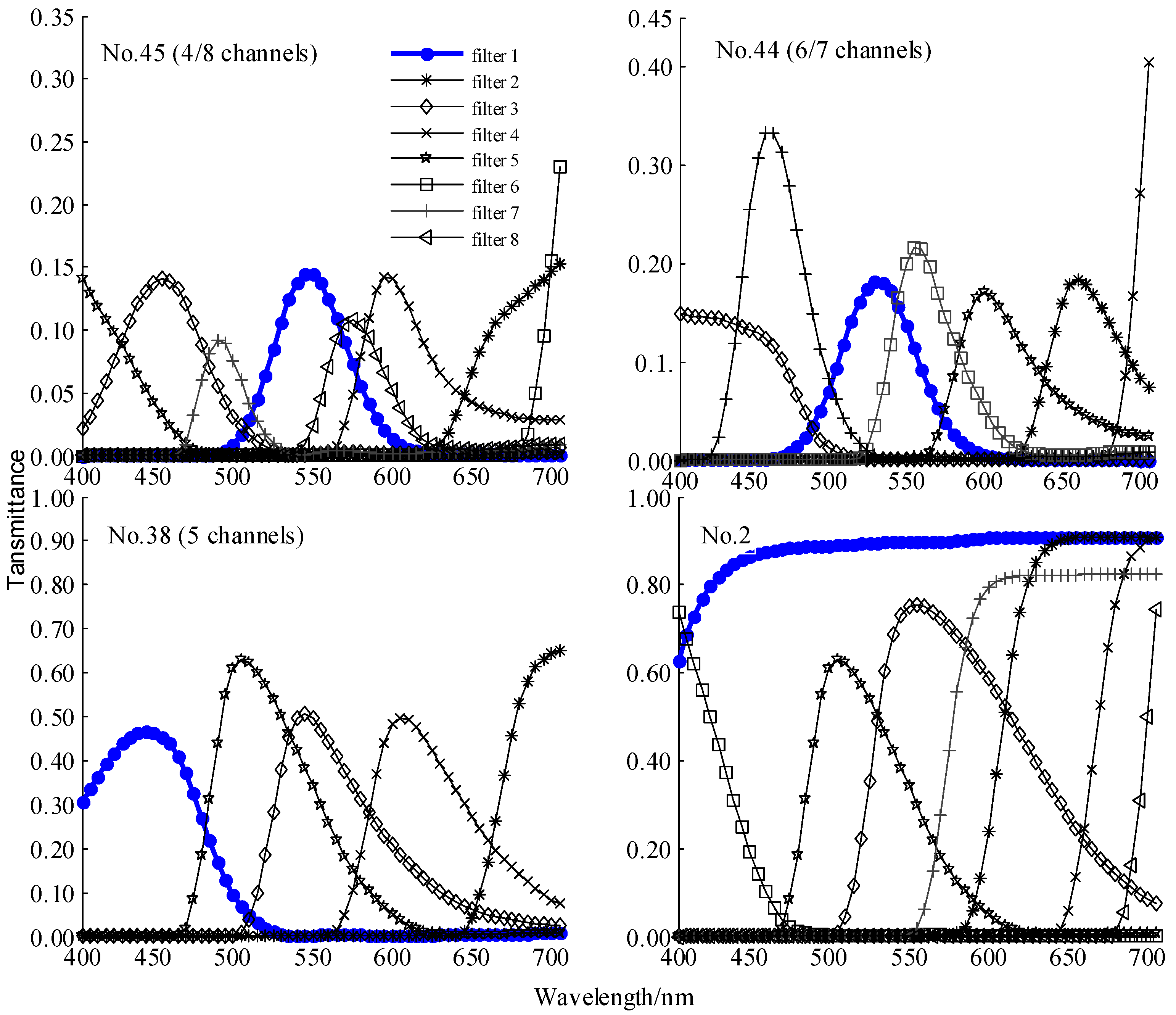
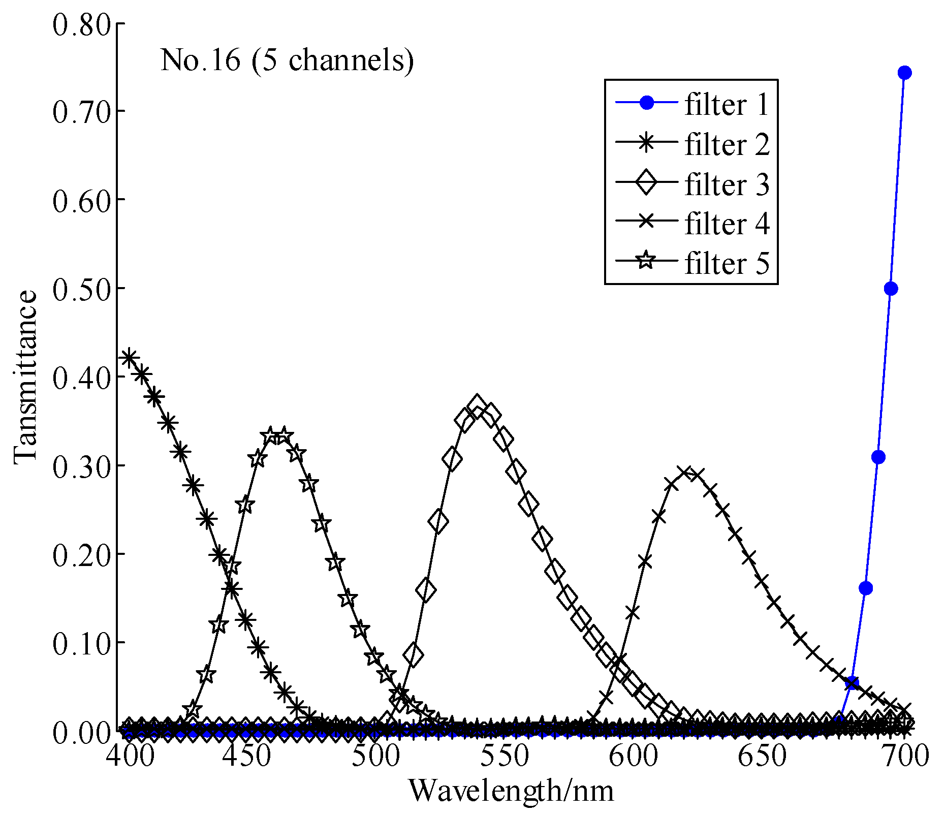
4.3.2. Transmittance Curves
5. Discussion
5.1. General Applicability of the MLI Method with Varying Imaging Parameters
5.2. Two Intuitive Steps for the MLI Method for Selecting Filter Sets
5.3. Possible Application and Future Work
6. Conclusions
Funding
Conflicts of Interest
References
- Li, S.; Zhang, L. Optimal sensitivity design of multispectral camera via broadband absorption filters based on compressed sensing. In Proceedings of the 3rd International Symposium of Space Optical Instruments and Applications, Beijing, China, 26–29 June 2016; Urbach, H., Zhang, G., Eds.; Springer: Cham, Switzerland, 2017; pp. 329–339. [Google Scholar]
- Shrestha, R.; Hardeberg, J.Y. Spectrogenic imaging: A novel approach to multispectral imaging in an uncontrolled environment. Opt. Express 2014, 22, 9123–9133. [Google Scholar] [CrossRef] [PubMed]
- Hardeberg, J.Y. Filter Selection for Multispectral Color Image Acquisition. J. Imaging Sci. Technol. 2004, 48, 177–182. [Google Scholar]
- Imai, F.H.; Quan, S.; Rosen, M.R.; Berns, R.S. Digital camera filter design for colorimetric and spectral accuracy. In Proceedings of the Third International Conference on Multispectral Color Science, Joensuu, Finland, 18–20 July 2001; University of Joensuu: Joensuu, Finland, 2001; pp. 23–26. [Google Scholar]
- Ng, D.Y.; Allebach, J.P. A subspace matching color filter design methodology for a multispectral imaging system. IEEE Trans. Image Process. 2006, 15, 2631–2643. [Google Scholar] [PubMed]
- Quan, S.; Ohta, N.; Katoh, N. Optimization of camera spectral sensitivities. In Proceedings of the Color and Imaging Conference; Society for Imaging Science and Technology: Springfield, VA, USA, 2000; pp. 273–278. [Google Scholar]
- Li, S.X.; Liao, N.F.; Sun, Y.N. Optimal Sensitivity of Multispectral imaging system based on PCA. Opto Electron. Eng. 2006, 33, 127–132. [Google Scholar]
- Wang, X.; Thomas, J.B.; Hardeberg, J.Y.; Gouton, P. Multispectral imaging: Narrow or wide band filters? J. Int. Colour Assoc. 2014, 12, 44–51. [Google Scholar]
- Vora, P.L.; Trussell, H.J. Measure of goodness of a set of color-scanning filters. J. Opt. Soc. Am. A 1993, 10, 1499–1503. [Google Scholar] [CrossRef]
- Hardeberg, J.Y. Acquisition and Reproduction of Color Image: Colorimetric and Multispectral Approaches; Universal-Publishers: Irvine, CA, USA, 2001; ISBN 1-58112-135-0. [Google Scholar]
- Li, S. Several Problems Research of Multispectral Imaging. PH.D. Thesis, Beijing Institute of Technology, Beijing, China, 2007. [Google Scholar]
- Arad, B.; Benshahar, O. Filter selection for hyperspectral estimation. In Proceedings of the IEEE Conference on Computer Vision and Pattern Recognition, ICCV, Beijing, China, 22–29 October 2017; pp. 3172–3180. [Google Scholar]
- Shrestha, R.; Hardeberg, J.Y. Multispectral imaging using LED illumination and an RGB camera. In Proceedings of the 23rd Color and Imaging Conference Final Program and Proceedings, Albuquerque, NM, USA, 4–8 November 2013; pp. 36–40. [Google Scholar]
- Lapray, P.J.; Wang, X.; Thomas, J.B.; Gouton, P. Multispectral Filter Arrays: Recent Advances and Practical Implementation. Sensors 2014, 14, 21626–21659. [Google Scholar] [CrossRef] [PubMed]
- Ansari, K.; Thomas, J.-B.; Gouton, P. Spectral band Selection Using a Genetic Algorithm Based Wiener Filter Estimation Method for Reconstruction of Munsell Spectral Data. Electron. Imaging 2017, 2017, 190–193. [Google Scholar] [CrossRef]
- Hirakawa, K.; Wolfe, P.J. Spatio-spectral color filter array design for optimal image recovery. IEEE Trans. Image Process. 2008, 17, 1876–1890. [Google Scholar] [CrossRef] [PubMed]
- Lu, Y.M.; Süsstrunk, S. Optimum spectral sensitivity functions for single sensor color imaging. In Digital Photography VIII; International Society for Optics and Photonics: Bellingham, WA, USA, 2012; pp. 872–886. [Google Scholar]
- Hoya Corporation USA Optics Division. Available online: http://www.hoyaoptics.com/color_filter (accessed on 26 January 2017).
- Maloney, L.T.; Wandell, B.A. Color constancy: A method for recovering surface spectral reflectance. J. Opt. Soc. Am. A 1986, 3, 29–33. [Google Scholar] [CrossRef] [PubMed]
- López-Alvarez, M.A.; Hernández-Andrés, J.; Valero, E.M.; Romero, J. Selecting algorithms, sensors, and linear bases for optimum spectral recovery of skylight. J. Opt. Soc. Am. A 2007, 24, 942–956. [Google Scholar] [CrossRef]
- Cao, X.; Yue, T.; Lin, X.; Lin, S.; Yuan, X.; Dai, Q.; Carin, L.; Brady, D.J. Computational Snapshot Multispectral Cameras: Toward dynamic capture of the spectral world. IEEE Signal Process. Mag. 2016, 33, 95–108. [Google Scholar] [CrossRef]
- Shen, H.L.; Yao, J.F.; Li, C.; Du, X.; Shao, S.J.; Xin, J.H. Channel selection for multispectral color imaging using binary differential evolution. Appl. Opt. 2014, 53, 634–642. [Google Scholar] [CrossRef] [PubMed]
- Romero, J.; García-Beltrán, A.; Hernández-Andrés, A. Linear bases for representation of natural and artificial illuminants. J. Opt. Soc. Am. A 1997, 14, 1007–1014. [Google Scholar] [CrossRef]
- MathWorks. Available online: https://cn.mathworks.com/help/ident/ref/goodnessoffit.html (accessed on 20 June 2017).
- Imai, F.H.; Rosen, M.R.; Berns, R.S. Comparative Study of Metrics for Spectral Match Quality. In Proceedings of the Conference on Colour in Graphics, Imaging, and Vision, Poitiers, France, 2–5 April 2002; pp. 492–496. [Google Scholar]
- López-Alvarez, M.A.; Hernández-Andrés, J.; Romero, J.; Jee, L.R. Designing a practical system for spectral imaging of skylight. Appl. Opt. 2005, 44, 5688–5695. [Google Scholar] [CrossRef] [PubMed]
- Goetz, A.F.; Vane, G.; Solomon, J.E.; Rock, B.N. Imaging spectrometry for Earth remote sensing. Science 1985, 228, 1147–1153. [Google Scholar] [CrossRef] [PubMed]
- Valero, E.M.; Hu, Y.; Hernández-Andrés, J.; Eckhard, T.; Nieves, J.L.; Romero, J. Comparative performance analysis of spectral estimation algorithms and computational optimization of a multispectral imaging system for print inspection. Color Res. Appl. 2014, 39, 16–27. [Google Scholar] [CrossRef]
- Singh, T.; Singh, M. Disregarding spectral overlap: A unified approach for demosaicking, compressive sensing and color filter array design. In Proceedings of the 18th IEEE International Conference on Image Processing, Brussels, Belgium, 11–14 September 2011; pp. 3161–3164. [Google Scholar]
- Jean-Baptiste, T.; Pierre-Jean, L.; Pierre, G.; Cedric, C. Spectral Characterization of a Prototype SFA Camera for Joint Visible and NIR Acquisition. Sensors 2016, 16, 993. [Google Scholar] [CrossRef]
- Monno, Y.; Kitao, T.; Tanaka, M.; Okutomi, M. Optimal spectral sensitivity functions for a single-camera one-shot multispectral imaging system. In Proceedings of the 2012 19th IEEE International Conference on Image Processing (ICIP), Orlando, FL, USA, 30 September–3 October 2012; pp. 2137–2140. [Google Scholar]
- Mahmoudi Nahavandi, A.; Amani Tehran, M. A new manufacturable filter design approach for spectral reflectance estimation. Color Res. Appl. 2017, 4, 316–326. [Google Scholar] [CrossRef]


| PSNR | GFC | ||||||
| No. | H-mean | No. | H-min | No. | H-mean | No. | H-min |
| 45 | 37.68 | 45 | 25.10 | 34 | 0.9215 | 34 | 0.5347 |
| 44 | 35.87 | 43 | 21.73 | 45 | 0.8829 | 43 | 0.0649 |
| 43 | 35.74 | 11 | 20.54 | 43 | 0.8728 | 45 | 0.0193 |
| 11 | 35.55 | 36 | 20.22 | 44 | 0.8722 | 11 | −0.7395 |
| 36 | 34.78 | 2 | 18.56 | 16 | 0.8536 | 41 | −0.8475 |
| 12 | 34.75 | 7 | 18.04 | 40 | 0.7544 | 44 | −0.9224 |
| 13 | 34.49 | 13 | 18.00 | 41 | 0.7484 | 40 | −1.0018 |
| 28 | 34.34 | 8 | 17.95 | 32 | 0.7437 | 36 | −1.0851 |
| 40 | 33.83 | 41 | 17.87 | 31 | 0.7364 | 16 | −1.3993 |
| MSE | CIEDE2000 | ||||||
| Series No. | L-mean | No. | L-min | Series No. | L-mean | No. | L-min |
| 45 | 2.20 | 33 | 5.68 | 45 | 4.67 | 42 | 0.09 |
| 43 | 4.43 | 38 | 6.27 | 43 | 5.13 | 35 | 0.10 |
| 11 | 5.06 | 35 | 6.33 | 38 | 6.88 | 38 | 0.11 |
| 36 | 6.14 | 42 | 6.33 | 13 | 6.94 | 33 | 0.13 |
| 44 | 7.84 | 45 | 6.40 | 44 | 6.98 | 26 | 0.14 |
| 12 | 8.22 | 3 | 6.41 | 11 | 7.04 | 27 | 0.14 |
| 13 | 8.69 | 27 | 6.48 | 36 | 7.15 | 1 | 0.14 |
| 28 | 9.66 | 26 | 6.49 | 12 | 7.67 | 5 | 0.15 |
| 2 | 1.08 | 5 | 6.52 | 28 | 7.77 | 3 | 0.15 |
| No. | Scores | No. | Scores | No. | Scores | No. | Scores | No. | Scores | No. | Scores |
|---|---|---|---|---|---|---|---|---|---|---|---|
| 4 channels | 5 channels | 6 channels | 7 channels | 8 channels | all channels | ||||||
| 45 | 43 | 38 | 48 | 44 | 57 | 44 | 50 | 45 | 57 | 45 | 56 |
| 43 | 42 | 16 | 42 | 45 | 41 | 35 | 47 | 34 | 31 | 43 | 46 |
| 38 | 33 | 44 | 39 | 11 | 37 | 38 | 38 | 12 | 31 | 11 | 30 |
| 16 | 31 | 45 | 31 | 16 | 36 | 45 | 32 | 28 | 29 | 44 | 28 |
| 36 | 30 | 13 | 30 | 40 | 30 | 43 | 27 | 33 | 28 | 38 | 22 |
| 13 | 27 | 35 | 20 | 43 | 27 | 34 | 22 | 43 | 28 | 36 | 22 |
| 29 | 23 | 34 | 18 | 42 | 21 | 33 | 18 | 13 | 24 | 34 | 18 |
| 35 | 23 | 40 | 14 | 33 | 19 | 25 | 16 | 27 | 23 | 42 | 15 |
| 44 | 16 | 43 | 13 | 34 | 16 | 27 | 14 | 42 | 15 | 35 | 15 |
| Indices | PSNR | GFC | MSE | DE2000 | ||||
|---|---|---|---|---|---|---|---|---|
| No. | 44 | 2 | 44 | 2 | 44 | 2 | 44 | 2 |
| 50db | 45.72 | 43.30 | 0.9984 | 0.9663 | 2.80 | 5.62 × 10⁻⁴ | 1.05 | 2.96 |
| 40db | 40.56 | 34.37 | 0.9897 | 0.8656 | 5.07 | 2.3 × 10⁻³ | 2.30 | 6.72 |
| 30db | 32.46 | 25.53 | 0.9139 | −0.0465 | 2.80 | 1.99 × 10⁻² | 6.22 | 16.26 |
| Channels | No. 45 | No. 38 | No. 44 | No. 2 |
|---|---|---|---|---|
| 4 | 1.45 | 1.65 | 1.37 | 5.84 |
| 5 | 2.11 | 2.56 | 1.63 | 6.65 |
| 6 | 2.55 | 3.21 | 2.31 | 9.74 |
| 7 | 3.04 | 3.91 | 3.10 | 12.01 |
| 8 | 3.62 | 92.35 | 20.34 | 13.99 |
| No./Channels | 45/4 | 38/5 | 44/6 | 44/7 | 45/8 |
|---|---|---|---|---|---|
| UF | 0.950 | 0.983 | 0.937 | 0.983 | 0.984 |
| OLP | 0.094 | 0.176 | 0.120 | 0.142 | 0.132 |
| No. | Scores | No. | Scores | No. | Scores | No. | Scores | No. | Scores |
|---|---|---|---|---|---|---|---|---|---|
| 4 channels | 5 channels | 6 channels | 7 channels | 8 channels | |||||
| 45 | 43 | 16 | 50 | 44 | 52 | 44 | 50 | 45 | 57 |
| 43 | 40 | 38 | 42 | 45 | 43 | 35 | 46 | 34 | 31 |
| 16 | 36 | 45 | 39 | 16 | 38 | 38 | 37 | 12 | 31 |
| 38 | 33 | 44 | 37 | 34 | 31 | 45 | 31 | 28 | 29 |
| Channels | 4 | 5 | 6 | 7 | 8 |
|---|---|---|---|---|---|
| Cond | 1.22 | 1.30 | 2.30 | 22.15 | 2.01 |
| Channels | 4 | 5 | 6 | 7 | 8 |
|---|---|---|---|---|---|
| Filter No. | 45 | 38 | 44 | 44 | 45 |
| D65 | 3 | 5 | 2 | 2 | 1 |
| Filter No. | 45 | 16 | 44 | 44 | 45 |
| A | 3 | 1 | 2 | 2 | 1 |
| S/N | ∞ | 50 | 47 | 43 | 40 | 37 | 33 | 30 | 27 | 23 |
|---|---|---|---|---|---|---|---|---|---|---|
| PNSR | 43.2 | 42.1 | 41.5 | 40.3 | 39.0 | 37.2 | 34.3 | 31.9 | 29.2 | 25.6 |
© 2018 by the author. Licensee MDPI, Basel, Switzerland. This article is an open access article distributed under the terms and conditions of the Creative Commons Attribution (CC BY) license (http://creativecommons.org/licenses/by/4.0/).
Share and Cite
Li, S.-X. Filter Selection for Optimizing the Spectral Sensitivity of Broadband Multispectral Cameras Based on Maximum Linear Independence. Sensors 2018, 18, 1455. https://doi.org/10.3390/s18051455
Li S-X. Filter Selection for Optimizing the Spectral Sensitivity of Broadband Multispectral Cameras Based on Maximum Linear Independence. Sensors. 2018; 18(5):1455. https://doi.org/10.3390/s18051455
Chicago/Turabian StyleLi, Sui-Xian. 2018. "Filter Selection for Optimizing the Spectral Sensitivity of Broadband Multispectral Cameras Based on Maximum Linear Independence" Sensors 18, no. 5: 1455. https://doi.org/10.3390/s18051455
APA StyleLi, S.-X. (2018). Filter Selection for Optimizing the Spectral Sensitivity of Broadband Multispectral Cameras Based on Maximum Linear Independence. Sensors, 18(5), 1455. https://doi.org/10.3390/s18051455