A Data-Gathering Scheme with Joint Routing and Compressive Sensing Based on Modified Diffusion Wavelets in Wireless Sensor Networks

Abstract
:1. Introduction
- Improved diffusion wavelets are used as the basis for data gathering, which makes full use of sensor nodes’ spatial correlations;
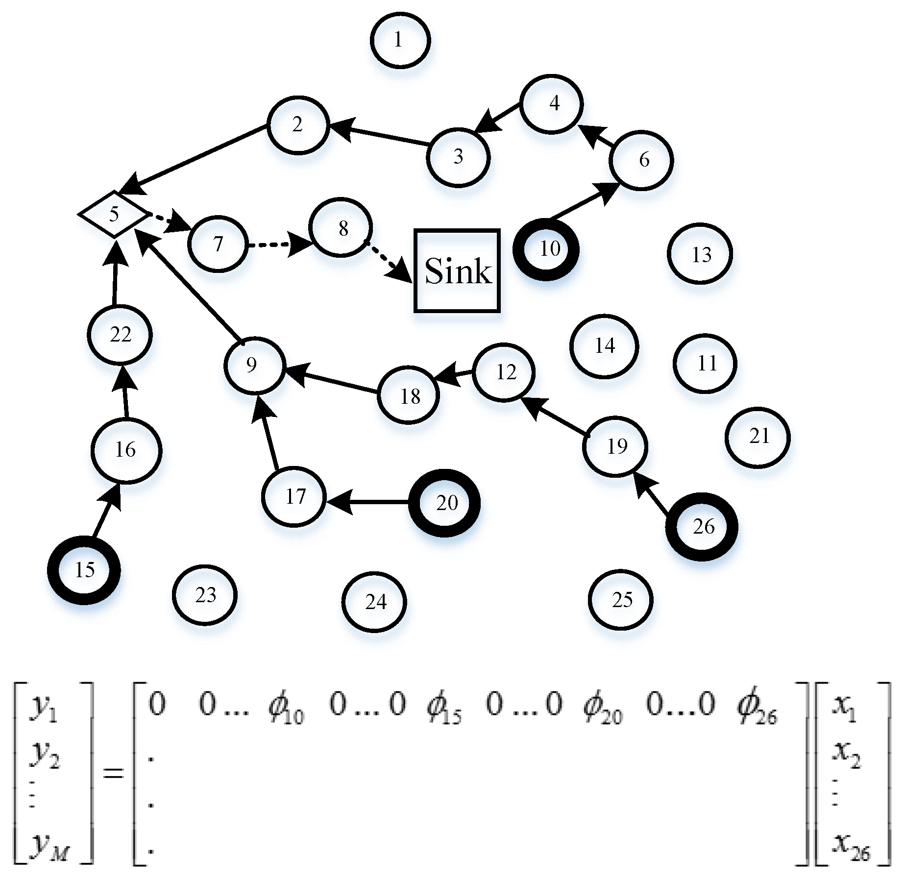
- A sparse measurement matrix is used, where the non-zero components of each row denote the offspring nodes of one projection node, which only requires a fraction of nodes to participate in each measurement task, leading to a dramatic decrease in the energy consumption.
- Modified ant colony routing compressively considering the next hop sensor node’s residual energy and path length is proposed; to speed up the algorithm coverage ratio and avoid a local optimal, the pheromone impact factor is improved. Furthermore, a novel data-gathering scheme that integrates MST (Minimum Spanning Tree), modified ant colony routing, and compressive sensing is provided;
- Theoretical proof is shown on the equivalent measurement matrix to satisfy the RIP.
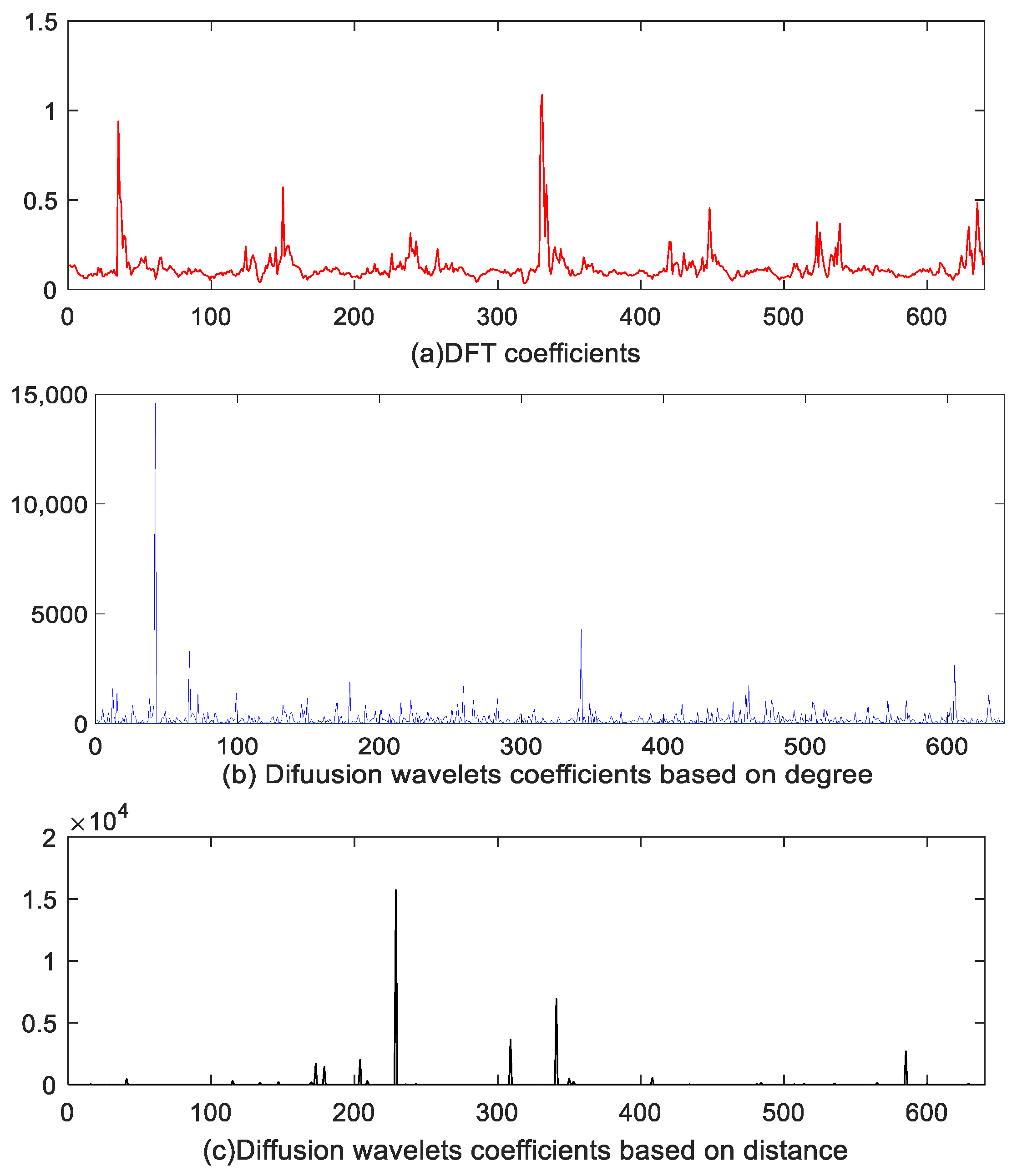
- The superiority of our approach is demonstrated by numerical experiments with synthetic and real sensor data. The simulations show that our sparse basis sparsity the signal. In addition, our approach can accurately reconstruct the original signal, thereby reducing the energy consumption of WSNs and balancing the network load.
2. Related Work
3. Preliminaries
3.1. CS Theory
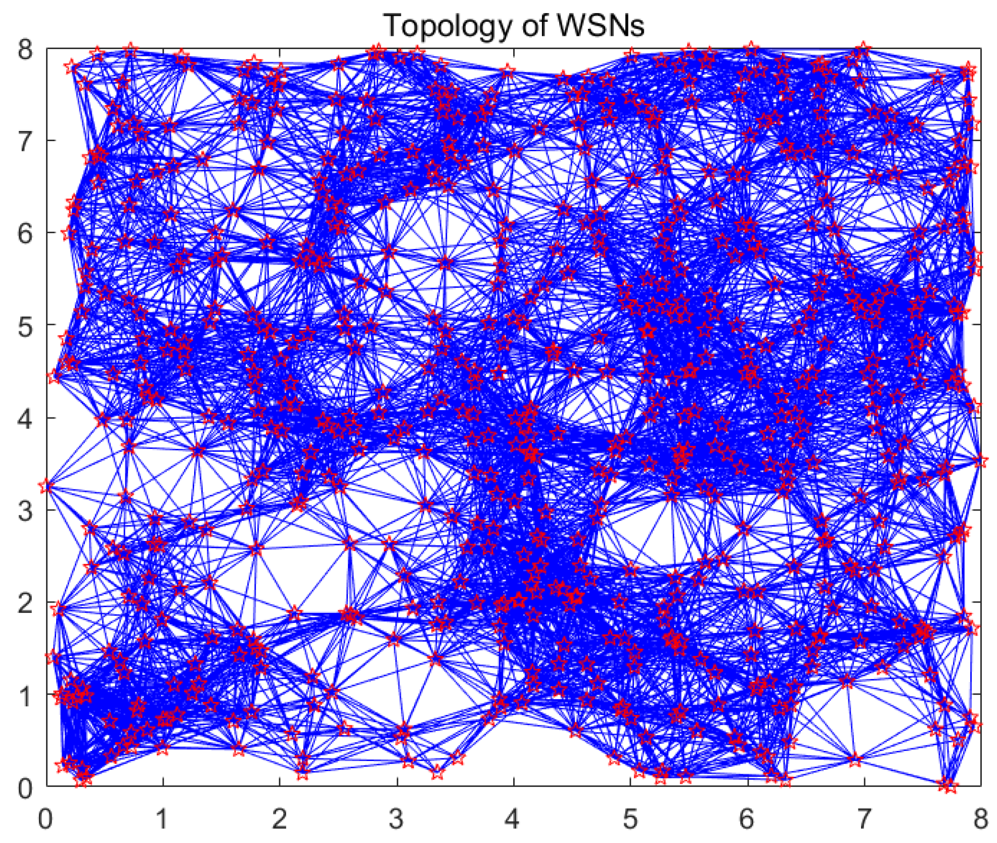
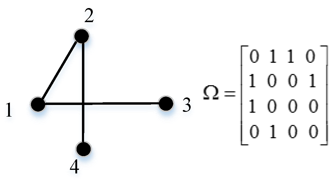
3.2. System Model
4. Our Proposed Algorithm
4.1. Datasets
4.1.1. Spatial Marginal and Conditional Entropy
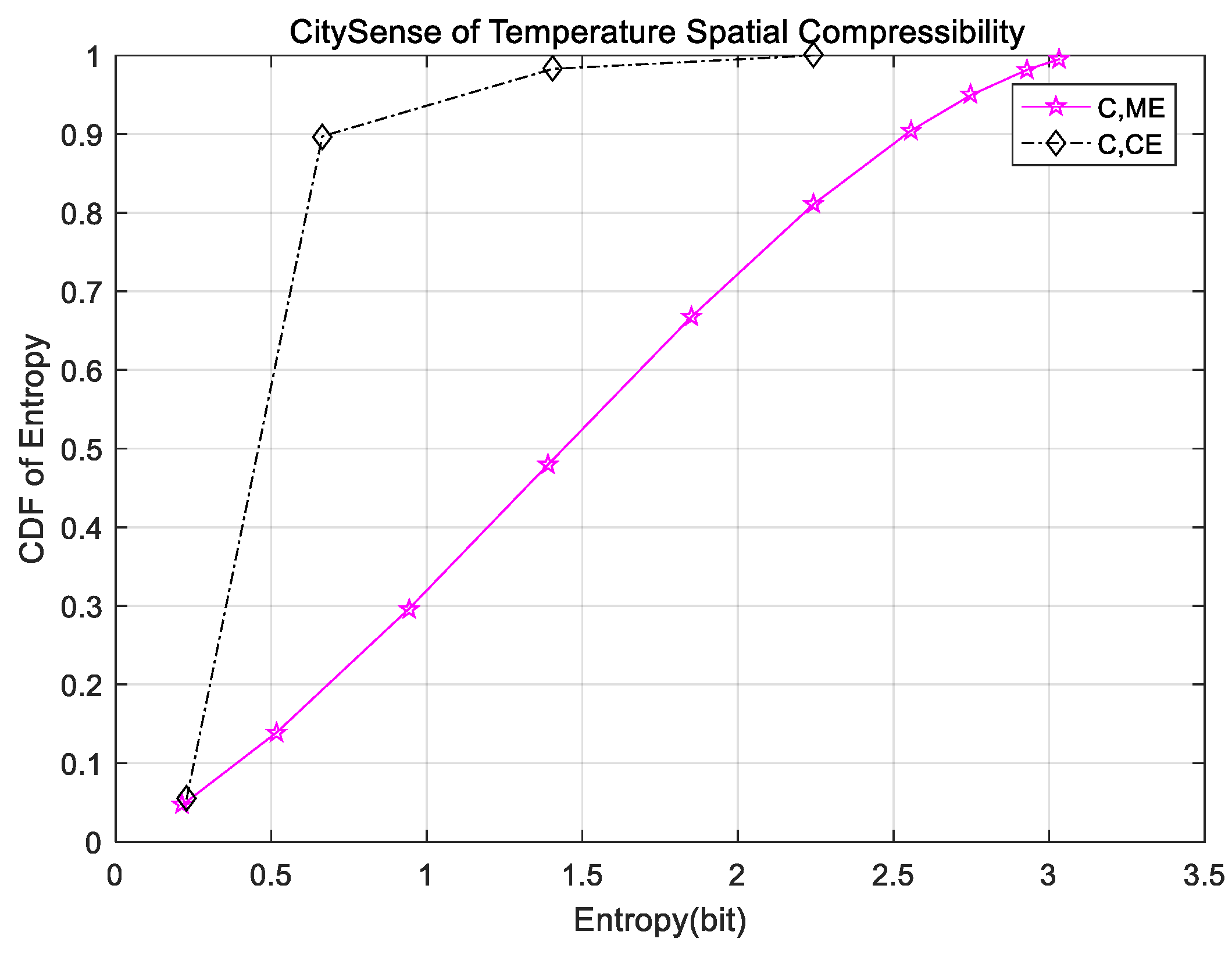
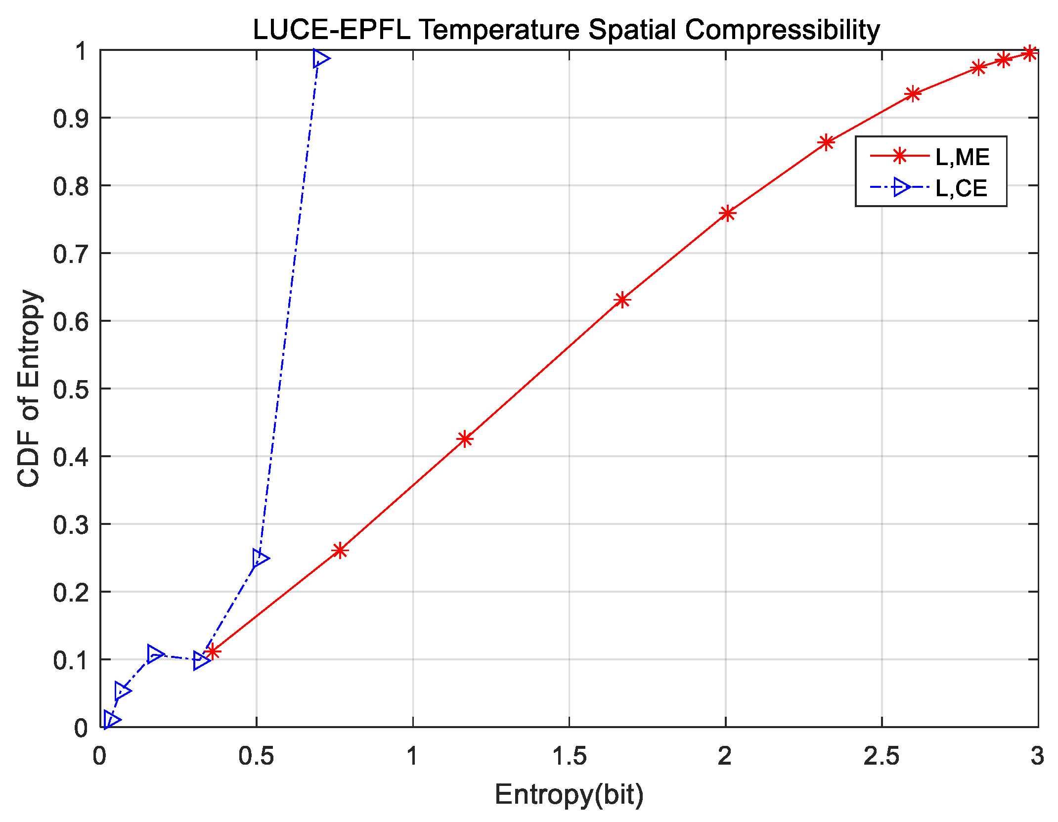
4.1.2. Spatial Compressibility
4.2. Modified Diffusion Wavelets
| Alogithm 1 Modified diffusion wavelets. |
| Input: the number of sensor nodes , communication radius , decomposition level , precision and MQR function. |
| Output: sparse basis . |
| 1 generate a graph |
| 2 compute weight adjacency matrix according to the vertex degree/Equation (11) |
| 3 calculate normalized Laplacian matrix relying on Equation (12)/Equation (13) |
| 4 generate diffusion operator |
| 5 recursively raising to power 2 |
| 5.1 for = 0 to − 1 |
| 5.2 , |
| 5.3 |
| 5.4 |
| 5.5 end for |
| 6 concatenation of the scale functions and wavelet functions is regarded as the sparse basis . |
| MQR Function: |
| Input: B: sparse matrix, |
| Output: , matrix, possibly sparse, such that |
| (1) is orthogonal |
| (2) is upper triangular up to a permutation |
| (3) The columns of -span the space spanned by the columns of B |
4.3. Modified Ant Colony Routing Algorithm
| Algorithm 2. Modified ant colony algorithm. |
| Input: the number of sensor nodes , the power expended to run the transmitter or receiver circuitry of sensor node , energy consumption of multi-path fading amplifier , energy consumption of free-space amplifier , distance threshold , impact factors of pheromone information , impact factors of heuristic information , is a small positive constant , pheromone information on edge , heuristic information on edge , and are constants. |
| Output: optimal routing . |
| 1 Initialization routing , energy for each node and tabu |
| 2 calculate distance of different nodes, |
| 3 while maximum iterations has not be reached |
| 4 for =1: |
| 5 compute according to the node communication radius. |
| 6 generate transition probability based on Equations (15) and (16) |
| 7 choose the next hop node, relying on , modify routing and tabu |
| 8 the destination node or not? If not, go back to step 2, or proceed to step 9 |
| 9 update the node residual energy based on Equations (5) and (6), routing depending on Equation (17) |
| 10 end for |
| 11 end while |
| 12 return the optimal routing . |
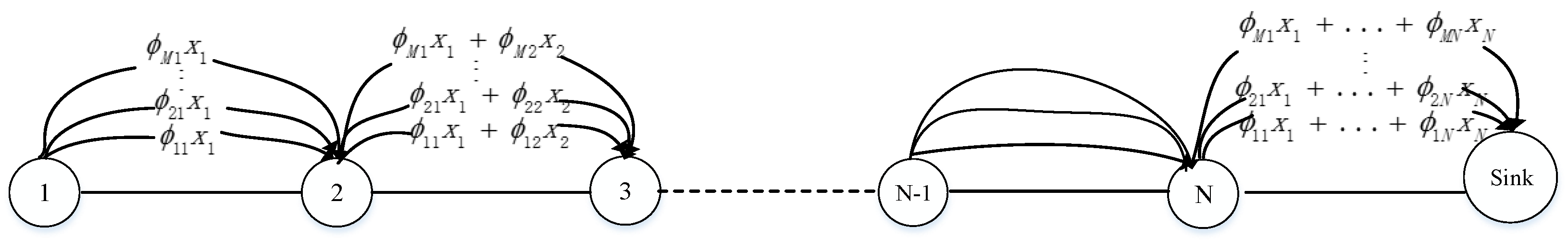
4.4. Compressive Data Gathering
4.5. Data Gathering with Sparse Random Projections
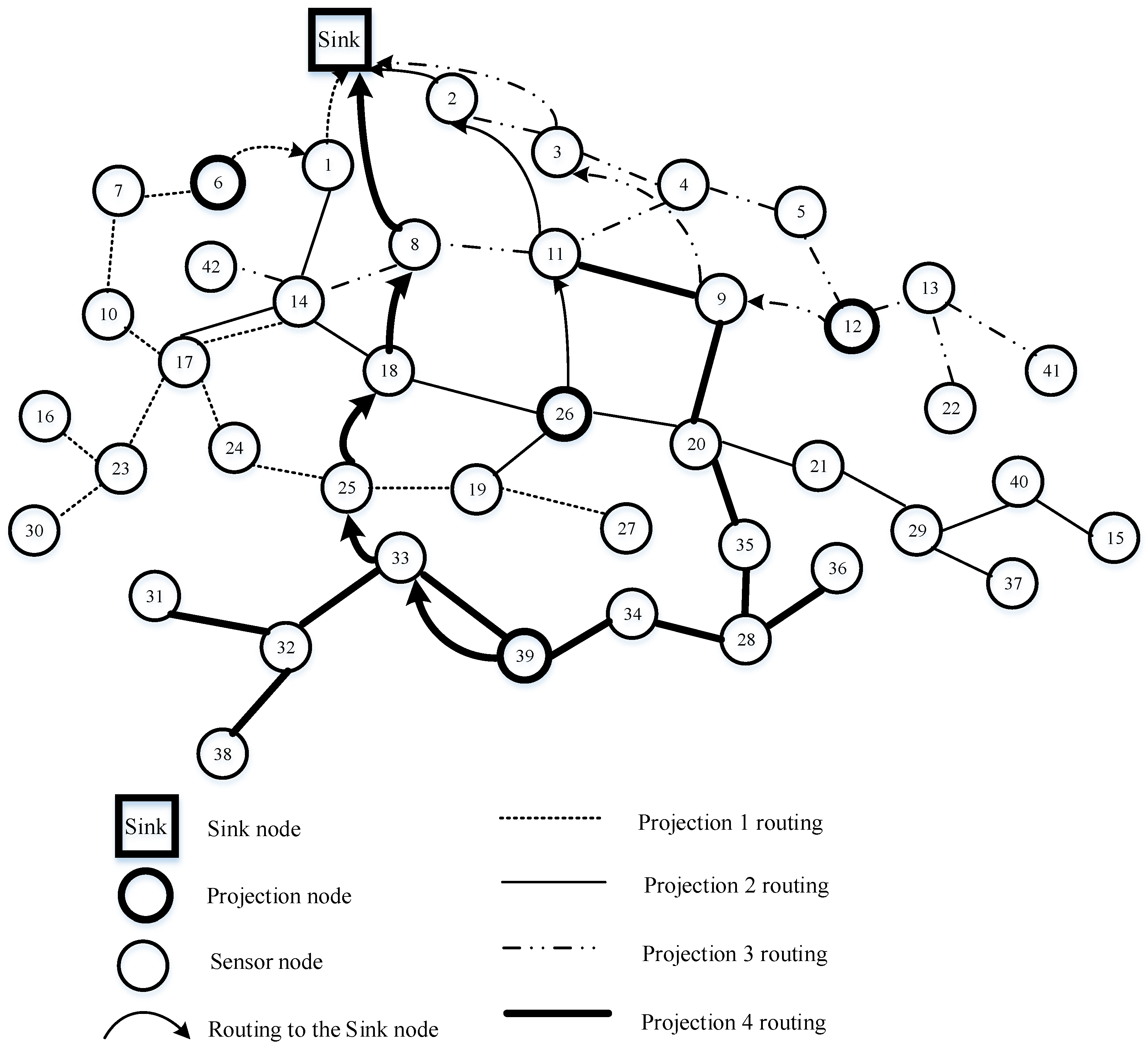
4.6. A Novel Data-Gathering Scheme with Joint Routing and CS
| Algorithm 3. Our proposed algorithm. |
| Input: |
| Output: , |
| 1 randomly select sensor nodes in the network probability , generate |
| 2 for |
| 3 query candidate nodes () of projection nodes |
| 4 initialization , |
| 5 while !empty(temp) do |
| 6 |
| 7 if is ’s candidate node |
| 8 |
| 9 |
| 10 |
| 11 end if |
| 12 end while |
| 13 while !empty() do |
| 14 for all residual candidate nodes |
| 15 find a shortest path to using the algorithm |
| 16 if > |
| 17 |
| 18 end if |
| 19 end for |
| 20 |
| 21 |
| 22 |
| 23 while !empty(temp) do |
| 24 go back to steps 7–11 |
| 25 end while |
| 26 end while |
| 27 Optimal routing from to the sink node using Algorithm 2 |
| 28 return |
| 29 end for |
| Algorithm 4. Sensor signal reconstruction. |
| 1 Input: received data , measurement matrix , the number of atom is |
| 2 Output: reconstruct data |
| 3 generate sparse basis using Algorithm 1 |
| 4 collect data in the network using Algorithm 3 |
| 5 |
| 6 initialization residual error , , , |
| 7 compute , select the largest values from ; these values correspond to ’s column indexes , constructing set |
| 8 set , (for all ) |
| 9 |
| 10 update |
| 11 , if go back to step 7, or proceed to step 12 |
| 12 reconstruct , which is the generation value of the last iteration . |
5. Theoretical Analysis
6. Simulation Results
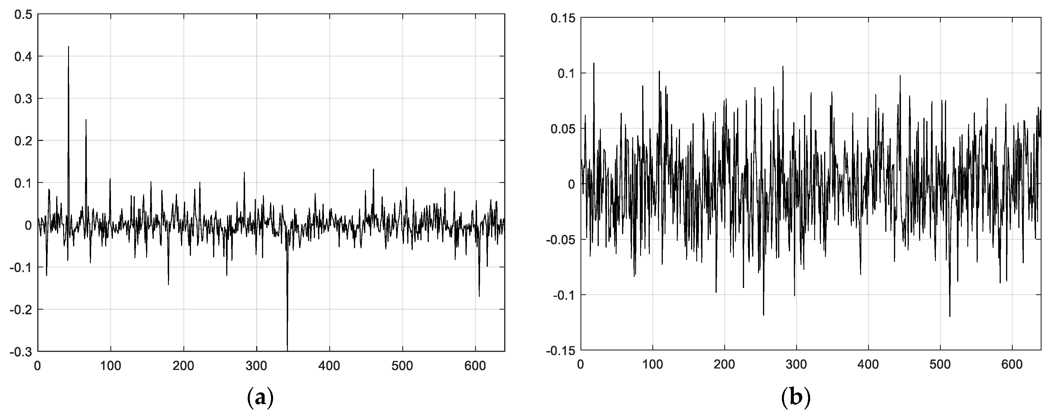
6.1. Sparse Comparison
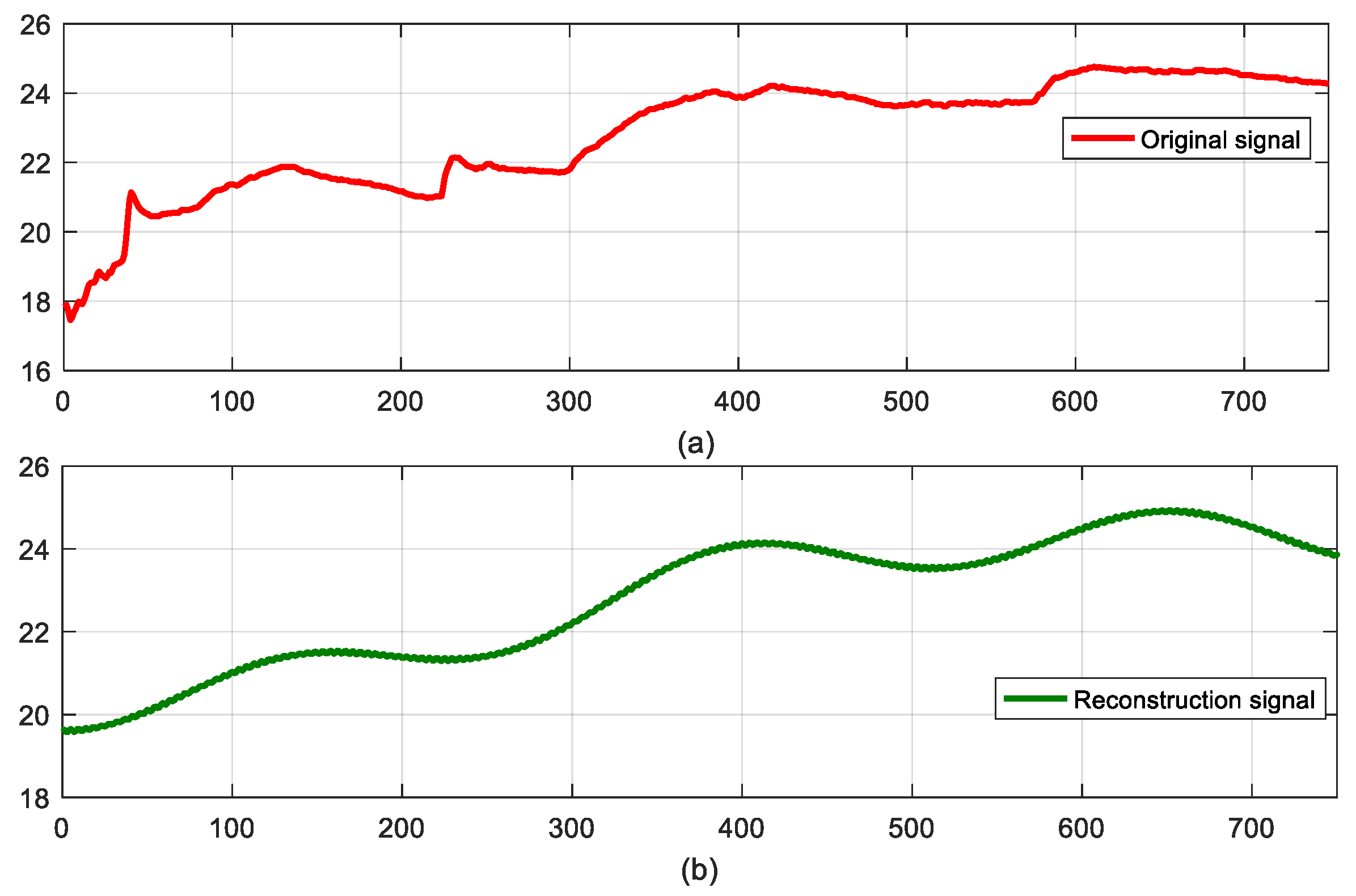
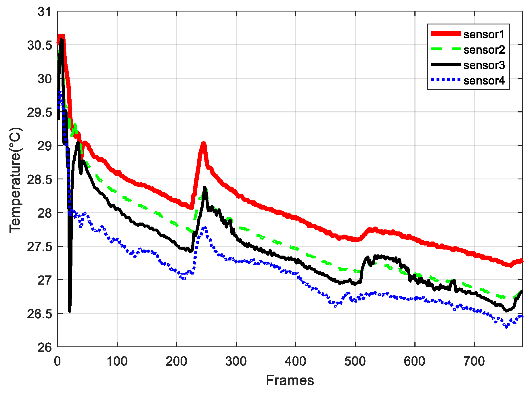
6.2. Performance of Reconstruction Signal
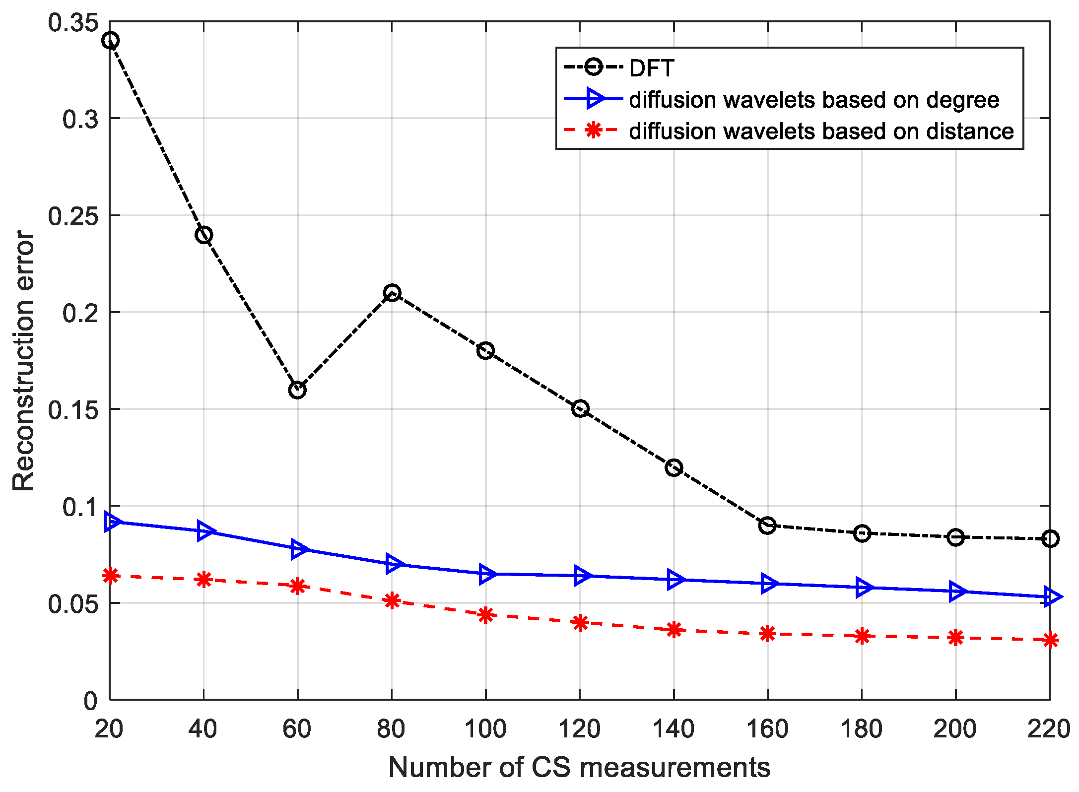
6.3. Reconstruction Error for Different Schemes
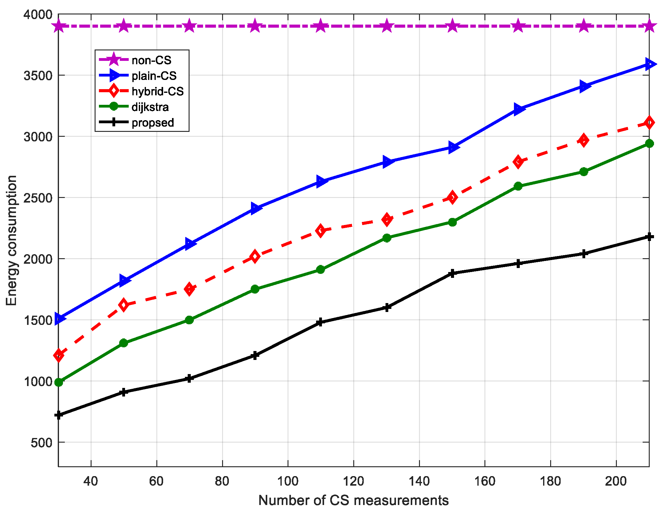
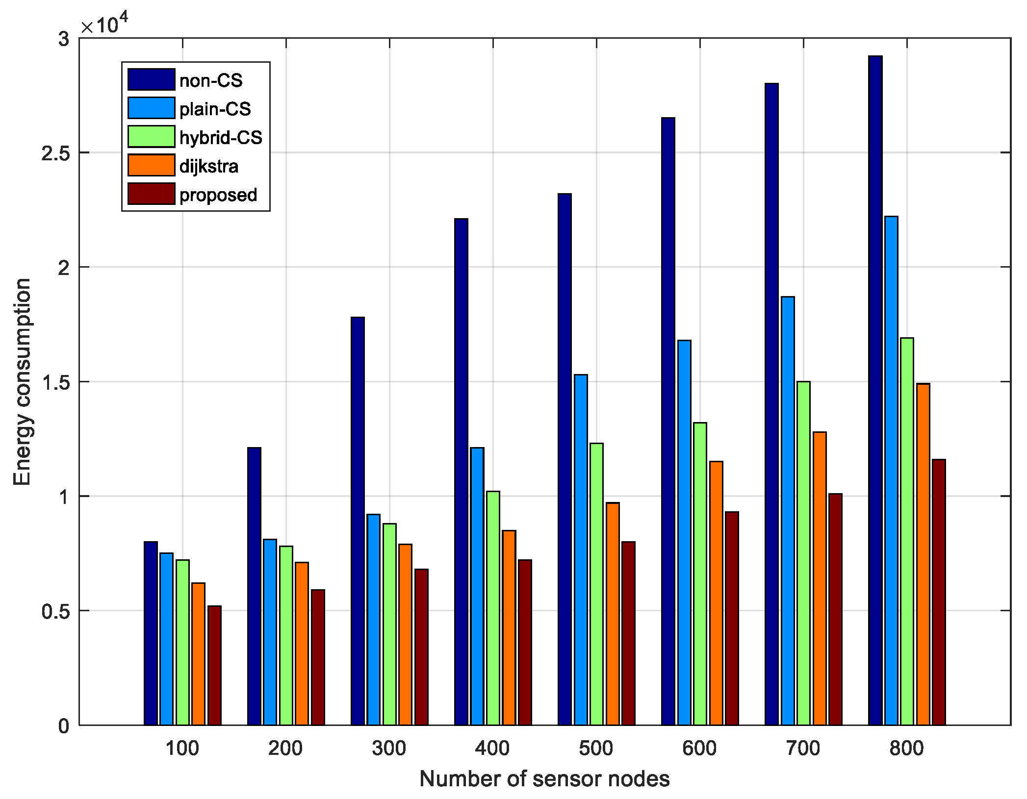
6.4. Energy Consumption Evaluation
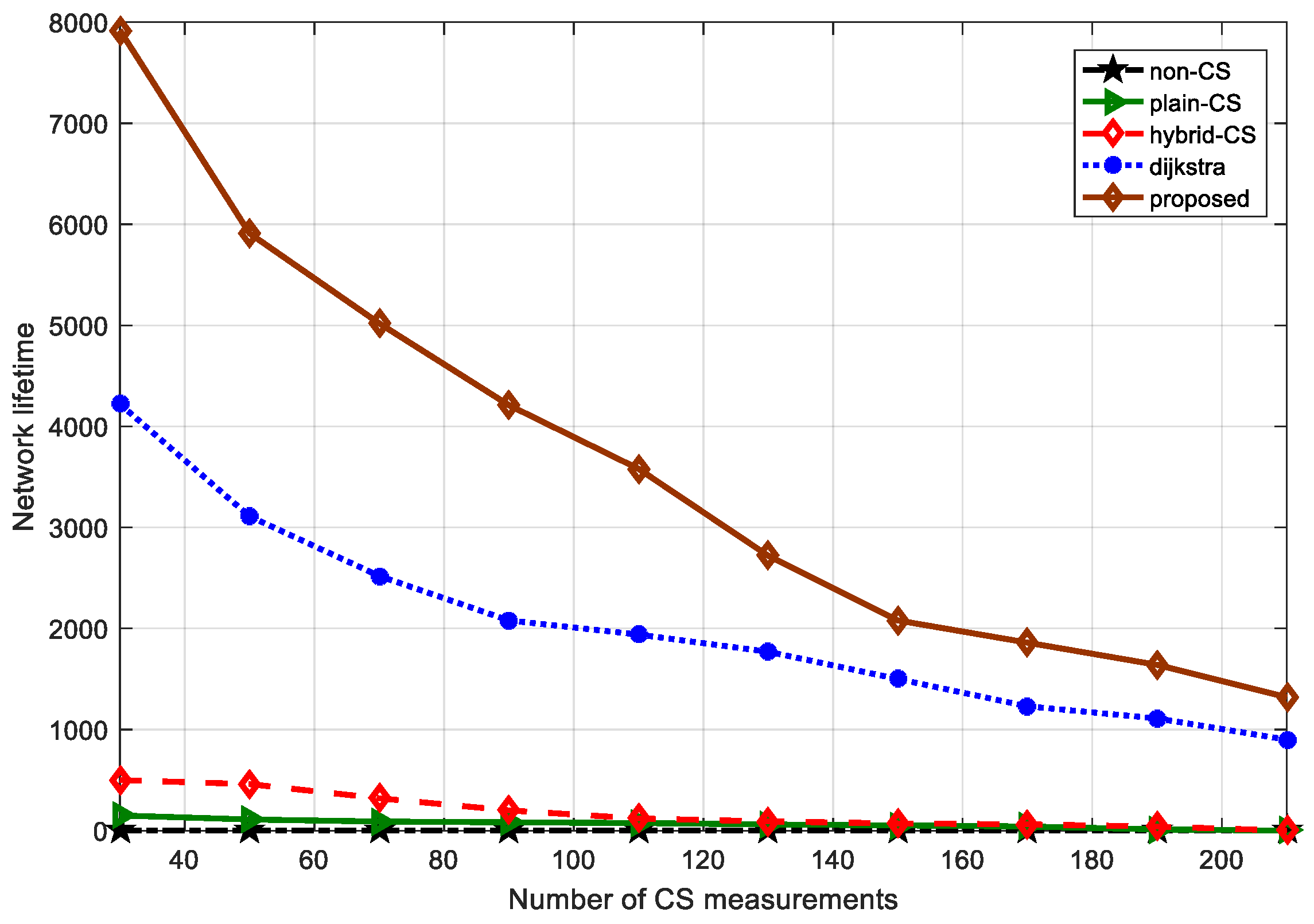
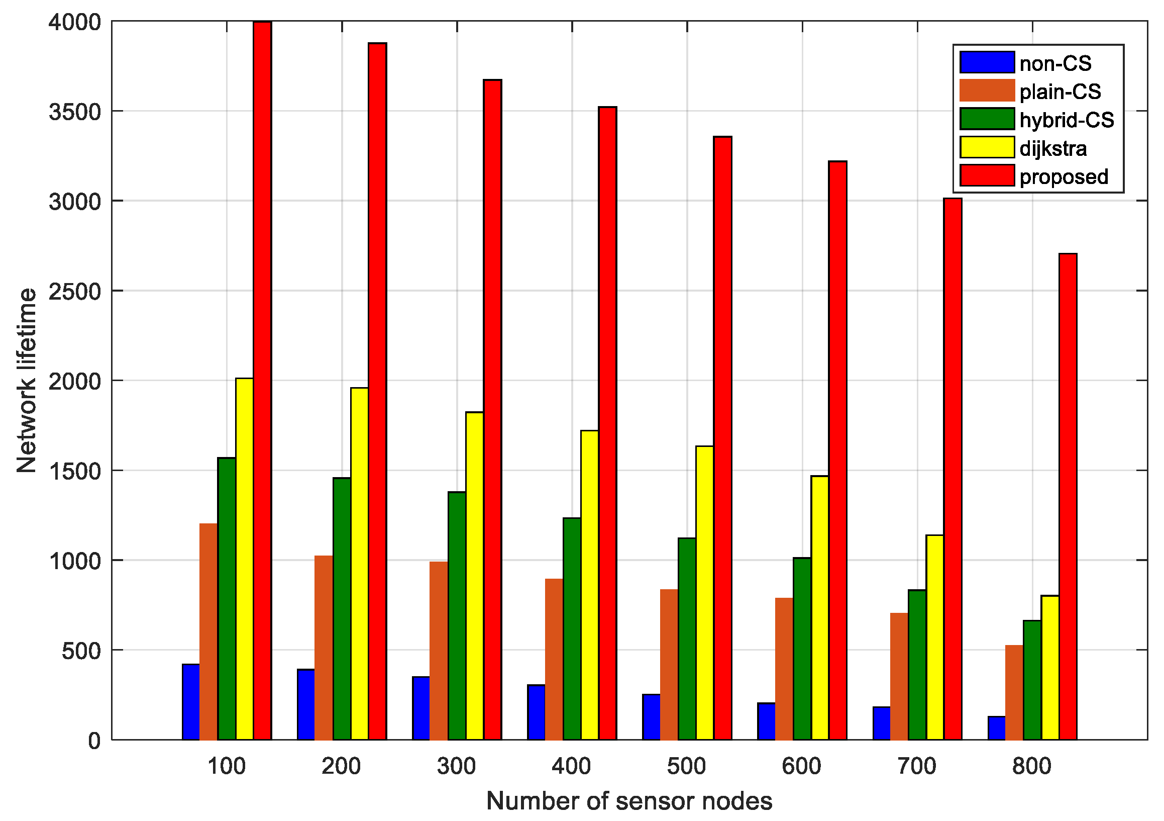
6.5. Network Lifetime Performance
7. Conclusions and Future Work
Acknowledgments
Author Contributions
Conflicts of Interest
References
- Anastasi, G.; Conti, M.; Francesco, M.D.; Passarella, A. Energy conservation in wireless sensor networks: A Survey. Ad Hoc Netw. 2009, 7, 537–568. [Google Scholar] [CrossRef]
- Hashemi, M.; Si, W.; Laifenfeld, M.; Starobinski, D.; Trachtenberg, A. Intra-car multihop wireless sensor networking: A case study. IEEE Commun. Mag. 2014, 52, 182–191. [Google Scholar] [CrossRef]
- Cheng, C.T.; Chi, K.T.; Lau, F.C.M. An energy-aware scheduling scheme for wireless sensor networks. IEEE Trans. Veh. Technol. 2010, 59, 3427–3444. [Google Scholar] [CrossRef]
- Aziz, A.A.; Sekercioglu, Y.A.; Fitzpatrick, P.; Ivanovich, M. A survey on distributed topology control techniques for extending the lifetime of battery powered wireless sensor networks. IEEE Commun. Surv. Tutor. 2013, 15, 121–144. [Google Scholar] [CrossRef]
- Wu, P.; Xiao, F.; Sha, C.; Huang, H.; Wang, R.; Xiong, N. Node scheduling strategies for achieving full-view area coverage in camera sensor networks. Sensors 2017, 17, 1303. [Google Scholar] [CrossRef] [PubMed]
- Zhao, M.; Ma, M.; Yang, Y. Efficient data gathering with mobile collectors and space-division multiple access technique in wireless sensor networks. IEEE Trans. Comput. 2011, 60, 400–417. [Google Scholar] [CrossRef]
- Li, X.; Tao, X.; Mao, G. Unbalanced expander based compressive data gathering in clustered wireless sensor networks. IEEE Access 2017, 5, 7553–7566. [Google Scholar] [CrossRef]
- Wang, Y.; Yang, Z.; Li, F.; Wen, H.; Shen, Y. CS2-collector: A new approach for data collection in wireless sensor networks based on two-dimensional compressive sensing. Sensors 2016, 16, 1318. [Google Scholar] [CrossRef] [PubMed]
- Candes, E.J.; Romberg, J.; Tao, T. Robust uncertainty principles: Exact signal reconstruction from highly incomplete frequency information. IEEE Trans. Inf. Theory 2006, 52, 489–509. [Google Scholar] [CrossRef]
- Donoho, D. Compressed sensing. IEEE Trans. Inf. Theory 2006, 52, 1289–1306. [Google Scholar] [CrossRef]
- Baraniuk, R. Compressive sensing. IEEE Signal Proc. Mag. 2007, 24, 118–121. [Google Scholar] [CrossRef]
- Luo, C.; Wu, F.; Sun, J.; Chen, C.W. Efficient measurement generation and pervasive sparsity for compressive data gathering. IEEE Trans. Wirel. Commun. 2010, 9, 3728–3738. [Google Scholar] [CrossRef]
- Talari, A.; Rahnavard, N. CStorage: Decentralized compressive data storage in wireless sensor networks. Ad Hoc Netw. 2016, 37, 475–485. [Google Scholar] [CrossRef]
- Wu, X.G.; Xiong, Y.; Wan, S.; Huang, W. Sparsest random scheduling for compressive data gathering in wireless sensor networks. IEEE Trans. Wirel. Commun. 2014, 13, 5867–5877. [Google Scholar] [CrossRef]
- Quer, G.; Masiero, R.; Pillonetto, G.; Rossi, M.; Zorzi, M. Sensing, compression, and recovery for wsns: Sparse signal modeling and monitoring framework. IEEE Trans. Wirel. Commun. 2012, 11, 3447–3461. [Google Scholar] [CrossRef]
- Salim, A.; Osamy, W. Distributed multi chain compressive sensing based routing algorithm for wireless sensor networks. Wirel. Netw. 2015, 21, 1379–1390. [Google Scholar] [CrossRef]
- Wang, X.; Zhao, Z.F.; Xia, Y. Compressed sensing for efficient random routing in multi-hop wireless sensor networks. Int. J. Commun. Netw. Distrib. Syst. 2011, 7, 275–292. [Google Scholar] [CrossRef]
- Zheng, H.F.; Yang, F.; Tian, X.; Gan, X.; Wang, X. Data Gathering with compressive sensing in wireless sensor networks: A random walk based approach. IEEE Trans. Parallel Distrib. Syst. 2015, 26, 35–44. [Google Scholar] [CrossRef]
- Xie, R.T.; Jia, X.H. Transmission-efficient clustering method for wireless sensor networks using compressive sensing. IEEE Trans. Parallel Distrib. Syst. 2014, 5, 806–815. [Google Scholar]
- Bajwa, W.; Haupt, J.; Sayeed, A.; Nowak, R. Compressive wireless sensing. In Proceedings of the 5th International Conference on Information Processing in Sensor Networks(IPSN), Nashville, TN, USA, 19–21 April 2006; pp. 134–142. [Google Scholar]
- Luo, J.; Xiang, L.; Rosenberg, C. Does compressed sensing improve the throughput of wireless sensor networks. In Proceedings of the IEEE International Conference on Communications, Cape Town, South Africa, 23–27 May 2010; pp. 1–6. [Google Scholar]
- Quer, G.; Masiero, R.; Munaretto, D.; Rossi, M. On the interplay between routing and signal representation for compressive sensing in wireless sensor networks. Inf. Theory Appl. Workshop 2009, 10, 206–215. [Google Scholar]
- Wang, W.; Garofalakis, M.; Ramchandran, K. Distributed sparse random projections for refinable approximation. In Proceedings of the 6th International Symposium on Information Processing in Sensor Networks(IPSN), Cambridge, MA, USA, 25–27 April 2007; pp. 331–339. [Google Scholar]
- Candès, E.; Romberg, J.; Tao, T. Decoding by linear programming. IEEE Trans. Inf. Theory 2005, 51, 4203–4215. [Google Scholar] [CrossRef]
- Tropp, J.A.; Gilbert, A.C. Signal recovery from random measurements via orthogonal matching pursuit. IEEE Trans. Inf. Theory 2007, 53, 4655–4666. [Google Scholar] [CrossRef]
- Needell, D.; Tropp, J.A. CoSaMP: Iterative signal recovery from incomplete and inaccurate samples. Appl. Comput. Harmon. Anal. 2009, 26, 301–321. [Google Scholar] [CrossRef]
- Donoho, D.L.; Tsaig, Y.; Drori, I.; Starck, J.L. Sparse solution of underdetermined systems of linear equations by stagewise orthogonal matching pursuit. IEEE Trans. Inf. Theory 2012, 58, 1094–1121. [Google Scholar] [CrossRef]
- Wang, J.; Kwon, W.; Shim, B. Generalized orthogonal matching pursuit. IEEE Trans. Signal Process. 2012, 60, 6202–6216. [Google Scholar] [CrossRef]
- Heinzelman, W.; Chandrakas, A.; Balakrishnan, H. Energy-efficient communication protocol for wireless sensor networks. In Proceedings of the 33rd Annual Hawaii International Conference on System Sciences, Maui, HI, USA, 4–7 January 2000; pp. 3005–3014. [Google Scholar]
- Thomas, M.C. Elements of Information Theory, 2nd ed.; Machinery Industry Press: Beijing, China, 2008; pp. 7–12. [Google Scholar]
- Casari, P.; Castellani, A.P.; Cenedese, A.; Lora, C.; Rossi, M.; Schenato, L.; Zorzi, M. The “wireless sensor networks for city-wide ambient intelligence (WISE-WAI)” project. Sensors 2009, 9, 4056–4082. [Google Scholar] [CrossRef] [PubMed]
- IntelLab. Available online: http://www.select.cs.cmu.edu/data/labapp3/index.html (accessed on 12 September 2016).
- EPFL LUCE SensorScope WSN. Available online: http://sensorscope.epfl.ch/ (accessed on 16 October 2017).
- CitySense. Available online: http://www.citysense.net (accessed on 18 October 2017).
- Watteyne, T.; Barthel, D.; Dohler, M.; Augeblum, I. Sense and sensitivity: A large-scale experimental study of reactive gradient routing. Meas. Sci. Technol. 2010, 21, 124001–124009. [Google Scholar] [CrossRef]
- Coifman, R.; Maggioni, M. Diffusion wavelets. Appl. Comput. Harmon. Anal. 2006, 21, 53–94. [Google Scholar] [CrossRef]
- Lv, C.; Wang, Q.; Yan, W.; Zhao, R. A sparse representation method of 2-D sensory data in wireless sensor networks. In Proceedings of the IEEE International Instrumentation and Measurement Technology Conference (I2MTC), Taipei, Taiwan, 23–26 May 2016; pp. 1–6. [Google Scholar]
- Chung, F. Spectral Graph Theory. In CBMS Regional Conference Series in Mathematics; American Mathematical Society: Providence, RI, USA, 1997; pp. 1–21. [Google Scholar]
- Dorigo, M.; Maniezzo, V.; Colorni, A. Ant system: Optimization by a colony of cooperating agents. IEEE Trans. Syst. Man Cybern. Part B 1996, 26, 29–41. [Google Scholar] [CrossRef] [PubMed]
- Dijkstra, E.W. A note on two problems in connexion with graphs. Numer. Math. 1959, 1, 269–271. [Google Scholar] [CrossRef]
- Davenport, M.A. Random Observation on Random Observations: Sparse Signal Acquisition and Processing. Ph.D. Thesis, Rice University, Houstion, TX, USA, 2010. [Google Scholar]
- Zordan, D.; Quer, G.; Zorzi, M.; Rossi, M. Modeling and Generation of Space-Time Correlated Signals for Sensor Network Fields. In Proceedings of the Global Telecommunications Conference, Houston, TX, USA, 5–9 December 2011; pp. 1–6. [Google Scholar]
- Elad, M. Optimized projection for compressed sensing. IEEE Trans. Signal Process. 2007, 55, 5695–5702. [Google Scholar] [CrossRef]


| Name | Time Period | Physical Signal | Matrix Size | Frame Length |
|---|---|---|---|---|
| LUCE-EPFL | 12–15 January 2007 | Temperature, Humidity, Solar Radiation, Wind, Water | 81 nodes × 856 | 5 min |
| IntelLab | 28 February 2004–5 April 2004 | Temperature, Humidity, Light, Voltage | 54 nodes × 500 | 30 s |
| CitySense | 14 October 2009–21 November 2009 | Temperature, Wind | 8 nodes × 887 | 60 min |
| DEI | 19–22 March 2009 | Temperature, Humidity, Light | 29 nodes × 781 | 5 min |
| OrangeLab | 26–27 August 2008 | Temperature, Light, Voltage | 75 nodes × 65 | 15 min |
| Name | Temperature | Humidity | Solar Radiation | Wind | Water | Light | Voltage |
|---|---|---|---|---|---|---|---|
| LUCE-EPFL | 2.971 | 2.810 | 2.450 | 2.484 | 2.991 | — | — |
| IntelLab | 2.543 | 1.629 | — | — | — | 2.151 | 1.015 |
| CitySense | 3.034 | — | — | 3.256 | — | — | — |
| DEI | 2.589 | 2.510 | — | — | — | 0.592 | — |
| OrangeLab | 2.832 | — | — | — | — | 1.193 | 1.836 |
© 2018 by the authors. Licensee MDPI, Basel, Switzerland. This article is an open access article distributed under the terms and conditions of the Creative Commons Attribution (CC BY) license (http://creativecommons.org/licenses/by/4.0/).
Share and Cite
Gu, X.; Zhou, X.; Sun, Y. A Data-Gathering Scheme with Joint Routing and Compressive Sensing Based on Modified Diffusion Wavelets in Wireless Sensor Networks. Sensors 2018, 18, 724. https://doi.org/10.3390/s18030724
Gu X, Zhou X, Sun Y. A Data-Gathering Scheme with Joint Routing and Compressive Sensing Based on Modified Diffusion Wavelets in Wireless Sensor Networks. Sensors. 2018; 18(3):724. https://doi.org/10.3390/s18030724
Chicago/Turabian StyleGu, Xiangping, Xiaofeng Zhou, and Yanjing Sun. 2018. "A Data-Gathering Scheme with Joint Routing and Compressive Sensing Based on Modified Diffusion Wavelets in Wireless Sensor Networks" Sensors 18, no. 3: 724. https://doi.org/10.3390/s18030724
APA StyleGu, X., Zhou, X., & Sun, Y. (2018). A Data-Gathering Scheme with Joint Routing and Compressive Sensing Based on Modified Diffusion Wavelets in Wireless Sensor Networks. Sensors, 18(3), 724. https://doi.org/10.3390/s18030724