A Novel Connectivity-Based LEACH-MEEC Routing Protocol for Mobile Wireless Sensor Network


Abstract
1. Introduction
- Mobile base station and mobile sensor nodes
- Mobile base station and static sensor nodes
- Static base station and mobile sensor nodes
- We propose LEACH-MEEC, where the connectivity and remaining energy of mobile sensor nodes are used as metrics for CL selection after the first round and onwards. This proposed metric significantly improves the performance as compared with the existing schemes.
- The proposed LEACH-MEEC is analyzed under different mobility models, using eight datasets with two different speed levels.
2. Related Work
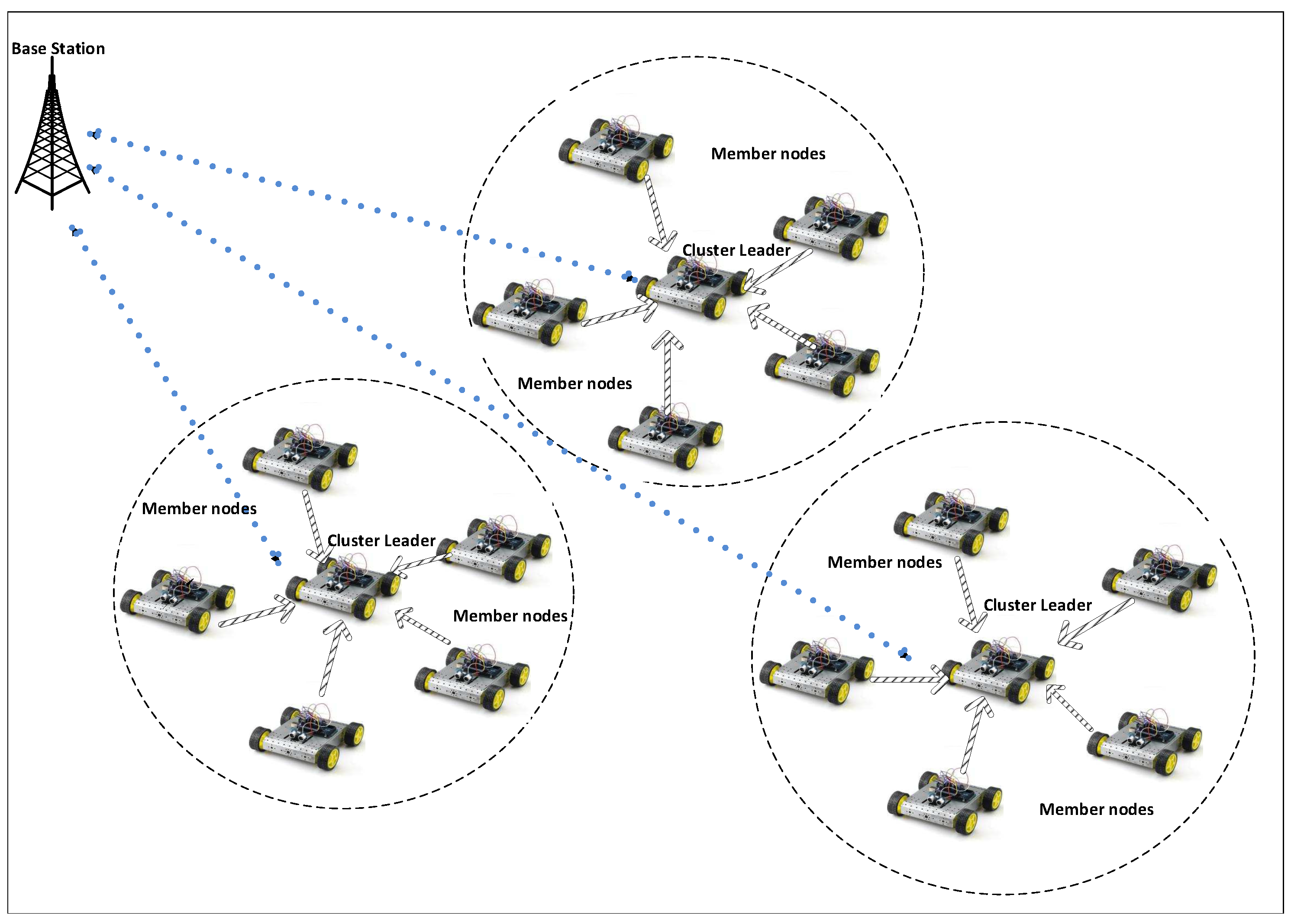
3. Proposed Framework
- Location of base station is anchored and positioned outside the area of sensors distribution.
- The N sensor nodes are distributed randomly.
- All sensors are homogeneous in nature, having similar specification.
- Mobile sensor nodes can move randomly with a specified speed following a certain mobility model pattern.
- Mobile sensor nodes can communicate directly with base station.
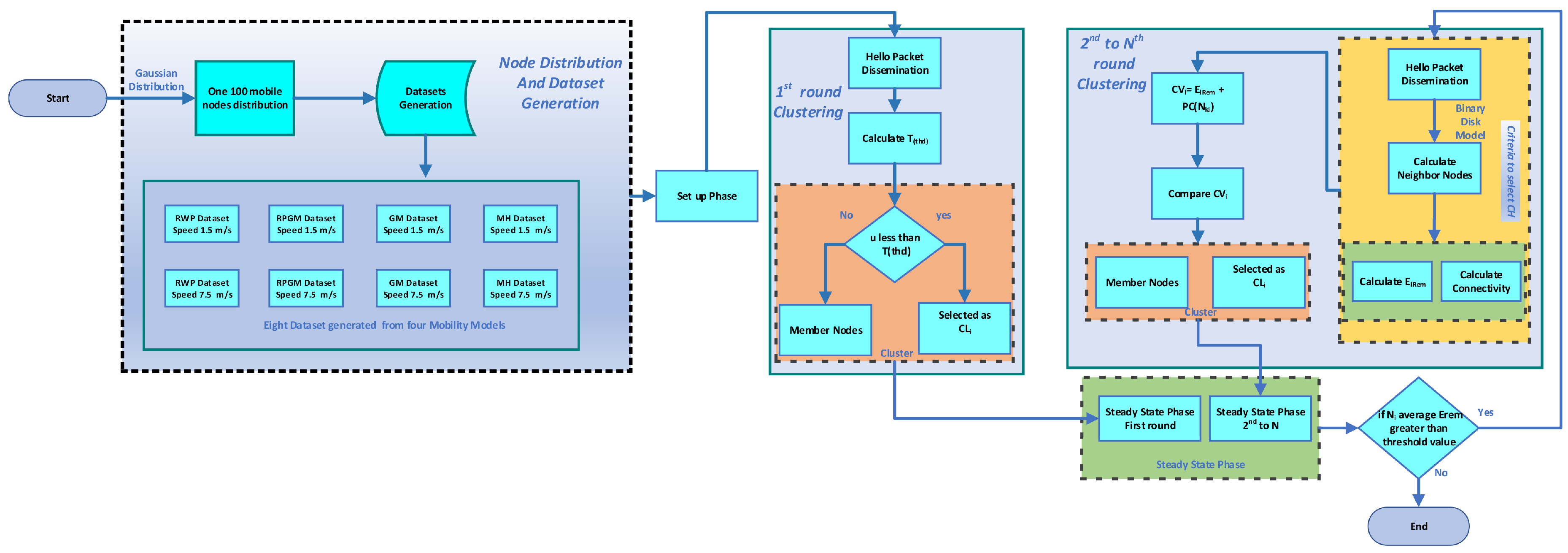
3.1. Mobile Sensor Distribution
3.2. Energy Model
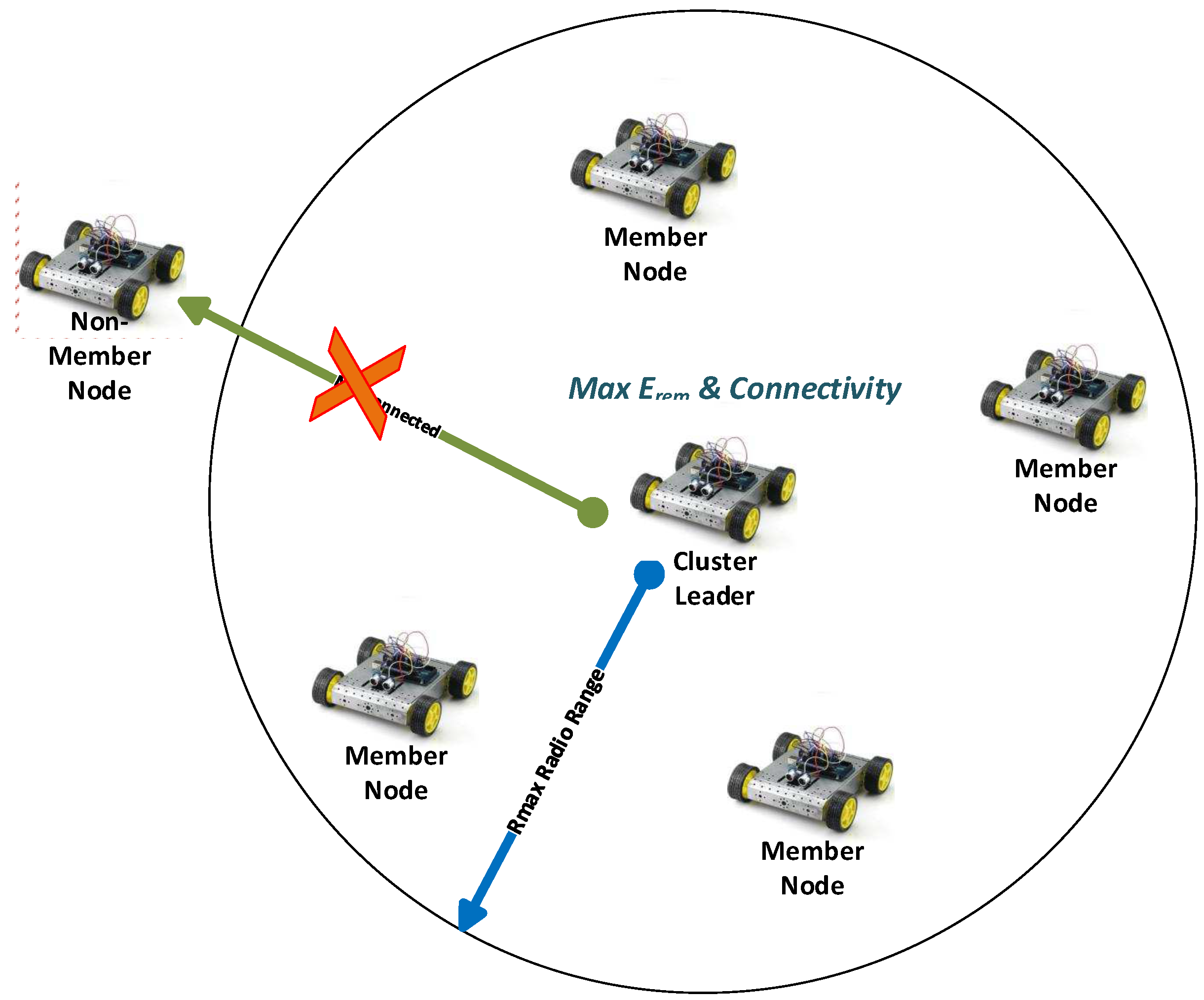
3.3. Connectivity
| Algorithm 1. Connectivity algorithm. |
 |
3.4. Cluster-Leader Election
4. Simulation Results and Discussion
4.1. Environment and Datasets
4.2. Experiments
- Time: The impact of different time duration ranging from 0 to 1000 s over the performance of LEACH-MEEC was studied.
- Number of Nodes: The impact of different numbers of nodes from 0 to 100 measuring the significance of packet delivery ratio over LEACH-MEEC was studied.
- Sensitivity Analysis: Different statistical estimation techniques were applied on results to measure the significance of connectivity feature over the performance of our algorithm to strengthen our claim.
4.3. Performance Metric
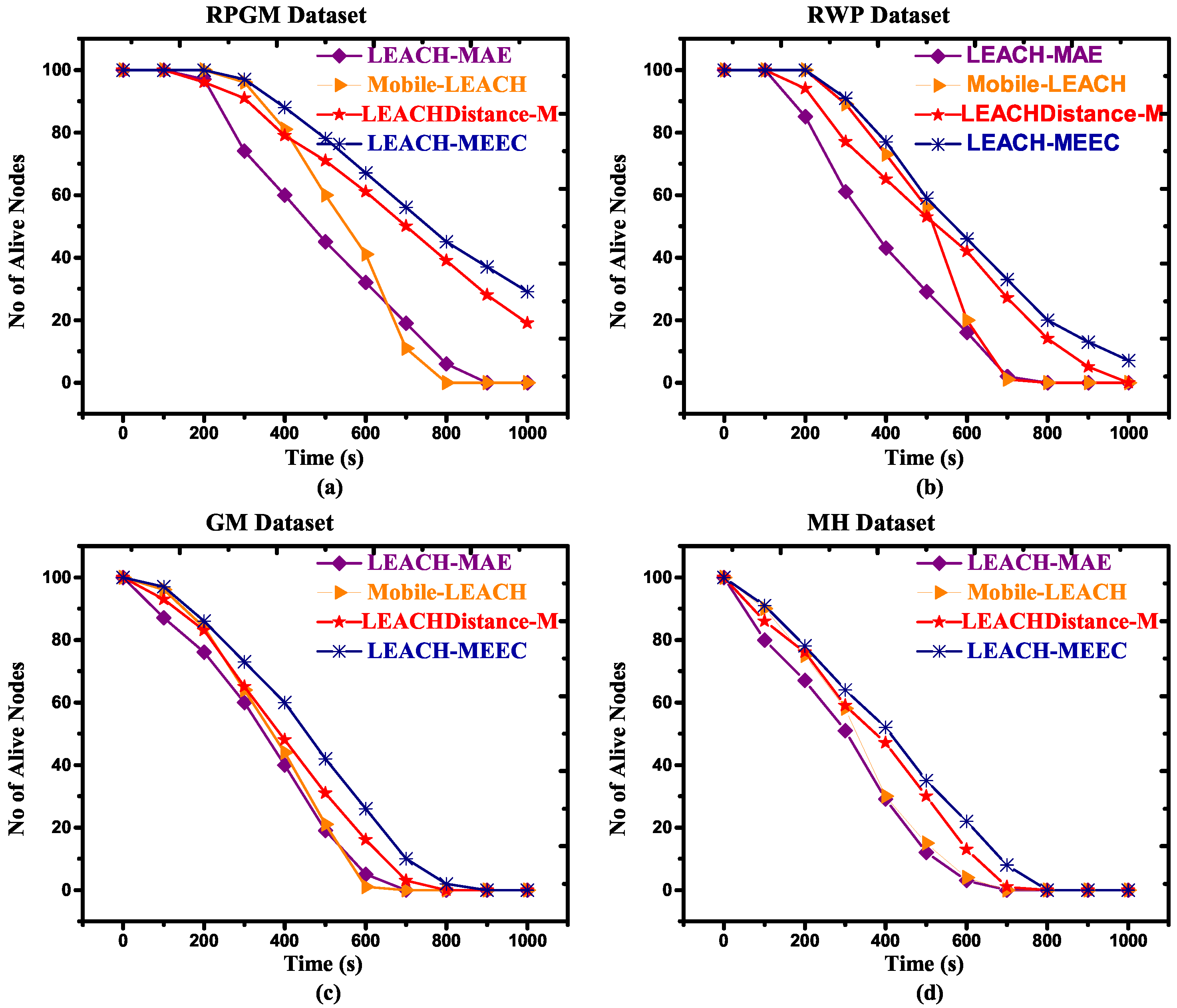
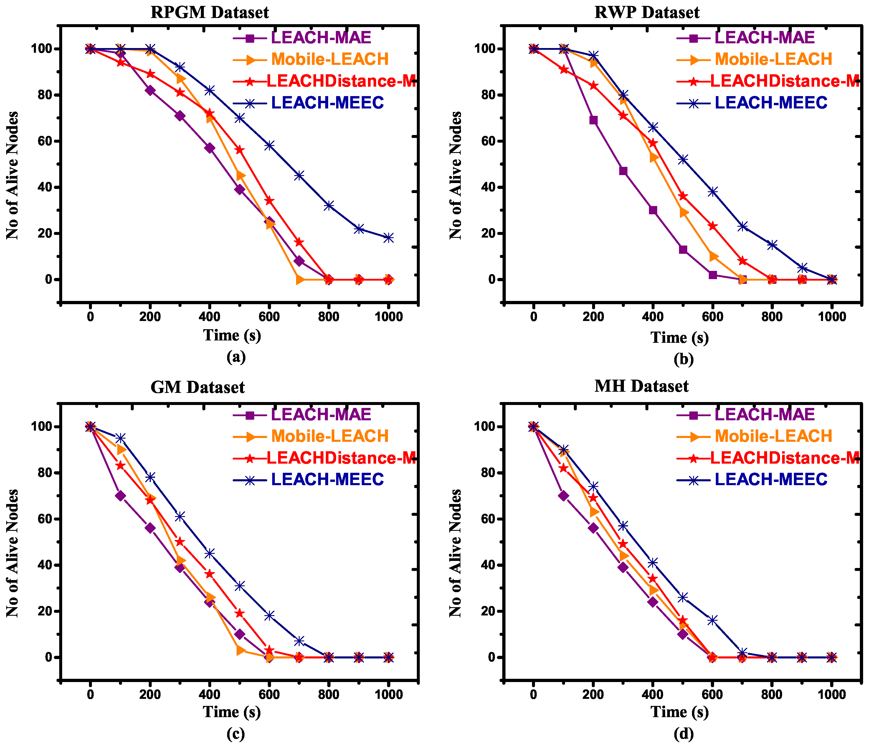
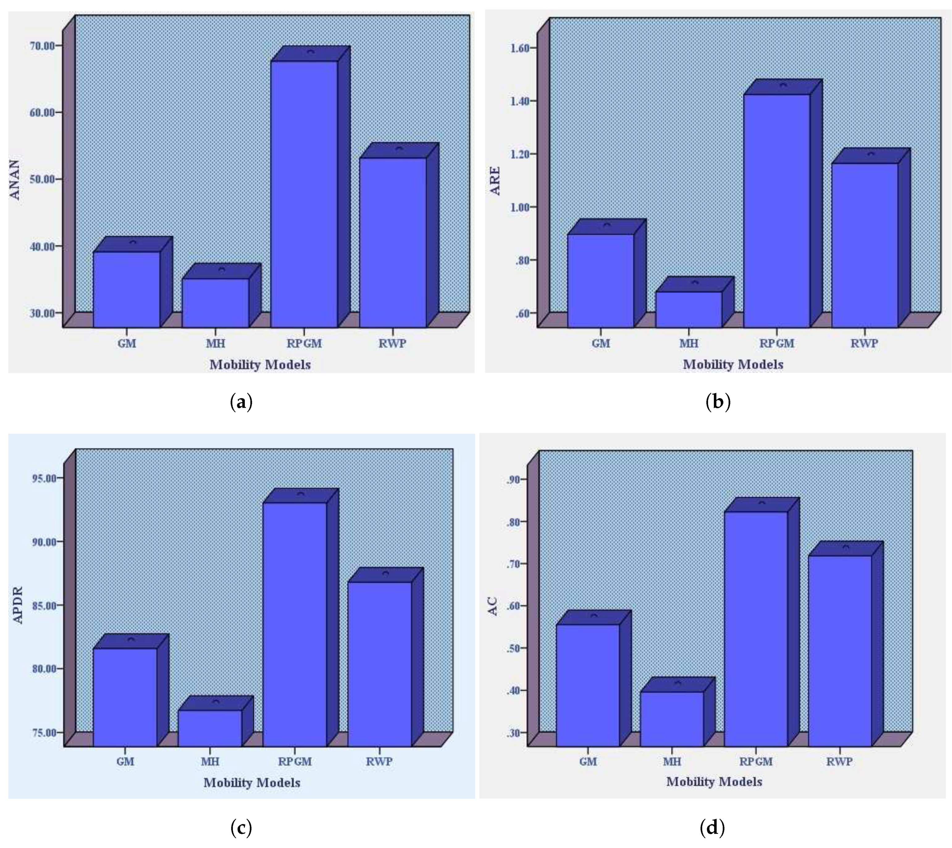
- Number of Alive Nodes (NAN): The number of remaining alive mobile sensor nodes after t seconds of simulation time was measured.
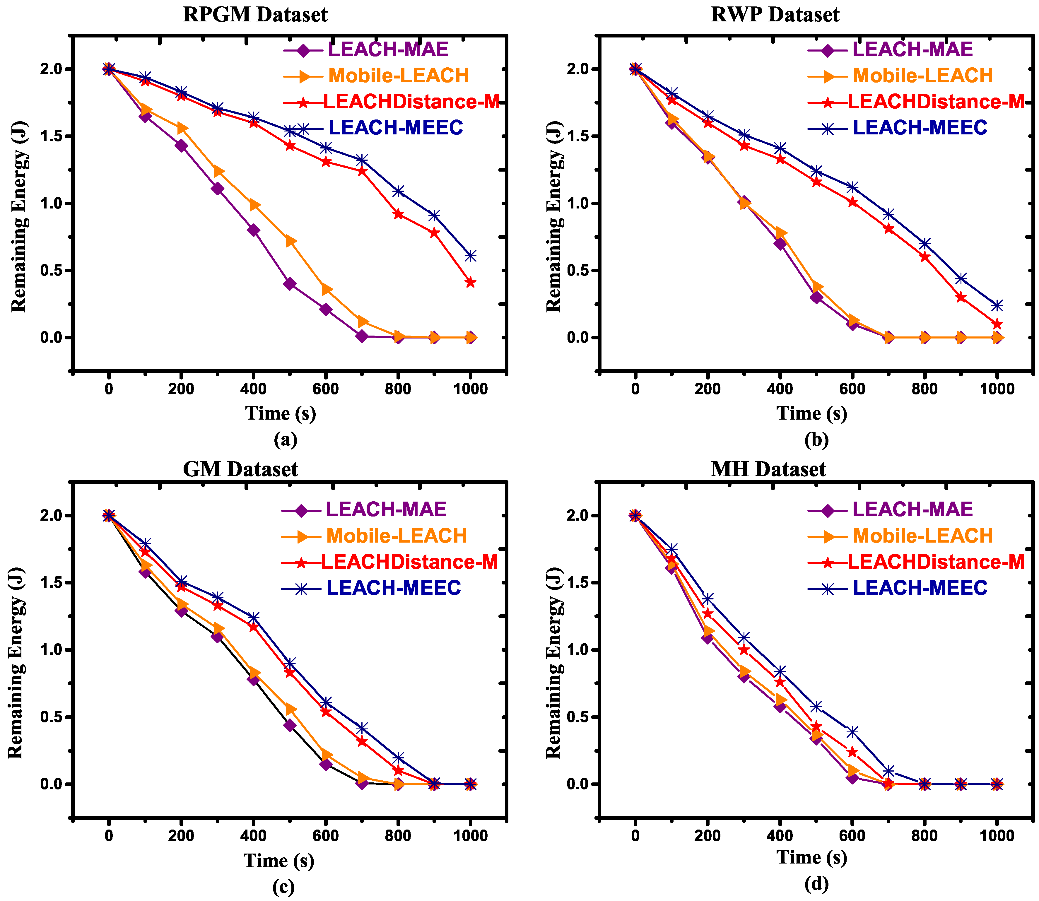
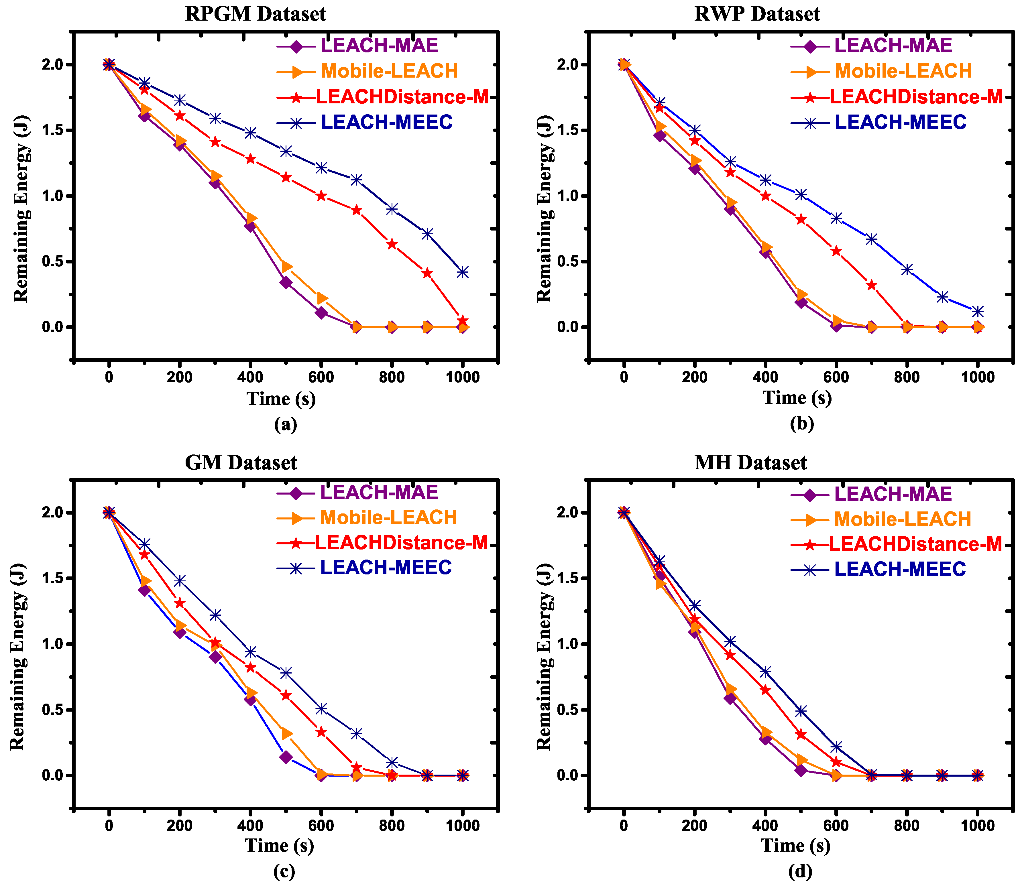
- Remaining Energy (RE): The average remaining energy (RE) of mobile sensor node at the end of each round was measured.
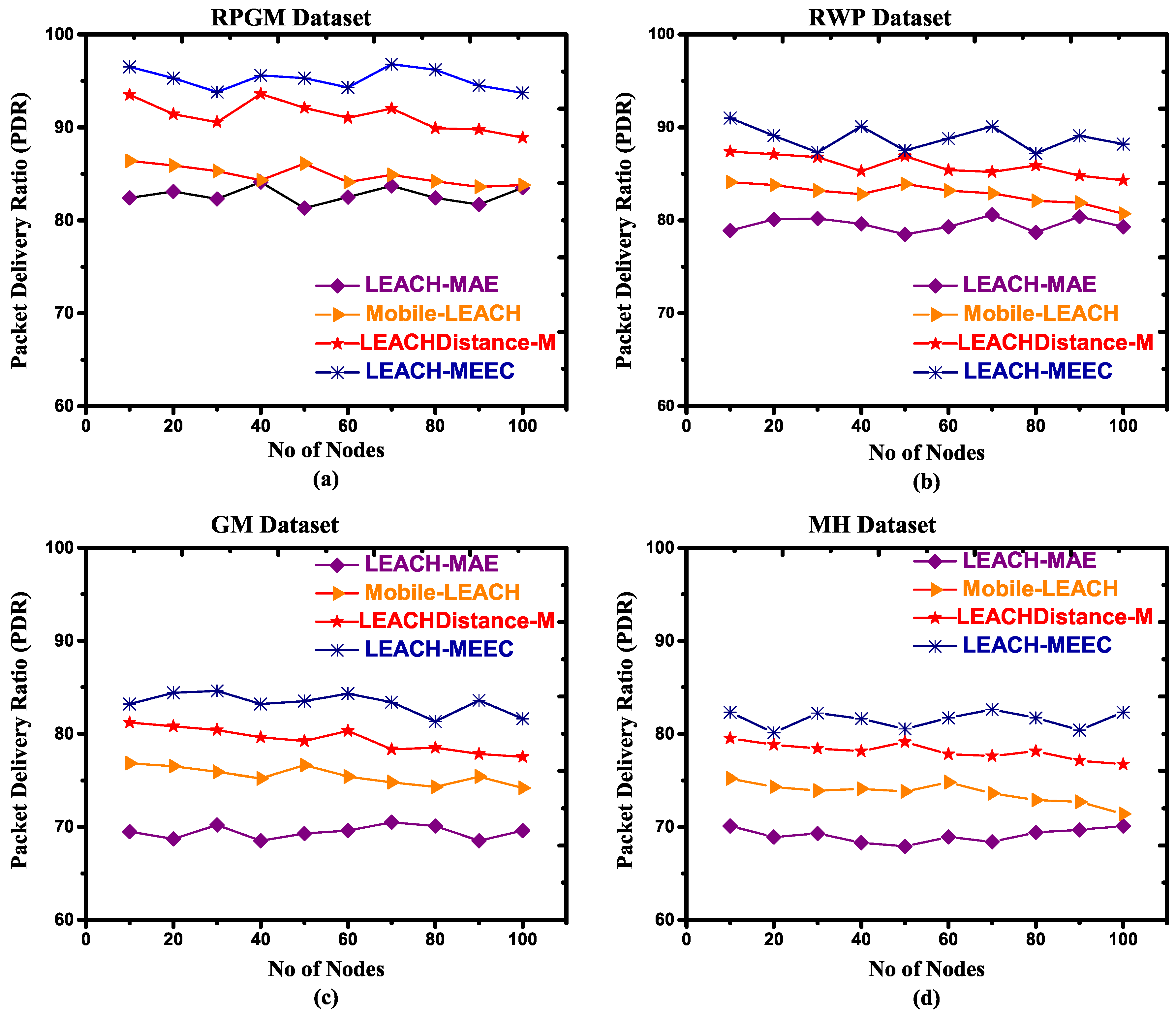
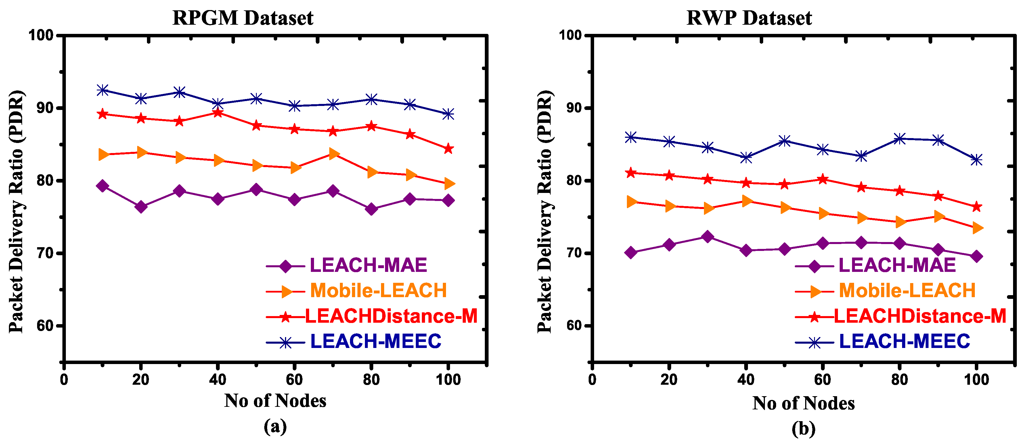
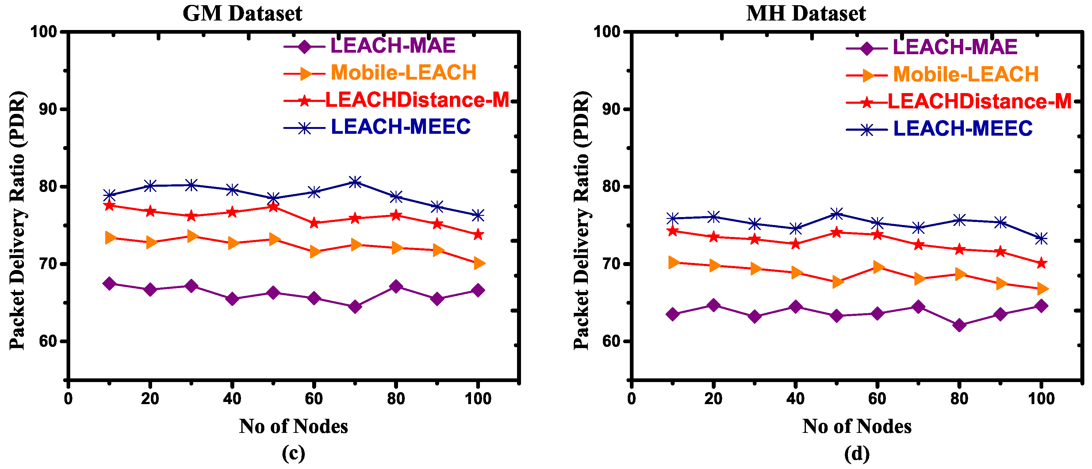
- Packet Delivery Ratio (PDR): Packet delivery ratio (PDR) is defined as the ratio between successful delivery of transmitted packets by a source (mobile sensor node) to a destination. The source mobile sensor node receives acknowledgment reply after successful delivery of packets at destination. The performance of protocol is considered better when PDR is high.Thus, we calculated the PDR with Equation (18).where PDR is packet delivery ratio, PRD is amount of packets received at destination, and PTS is amount of packets transmitted by source.
4.4. Results Discussion
4.4.1. Number of Alive Nodes (NAN)
4.4.2. Remaining Energy (RE)
4.4.3. Packet Delivery Ratio (PDR)
4.4.4. Sensitivity Analysis
5. Conclusions
Author Contributions
Funding
Conflicts of Interest
References
- Yue, Y.G.; He, P. A comprehensive survey on the reliability of mobile wireless sensor networks: Taxonomy, challenges, and future directions. Inf. Fusion 2018, 44, 188–204. [Google Scholar] [CrossRef]
- Ghasempour, A. Optimum number of aggregators based on power consumption, cost, and network lifetime in advanced metering infrastructure architecture for Smart Grid Internet of Things. In Proceedings of the 2016 13th IEEE Annual Consumer Communications Networking Conference (CCNC), Las Vegas, NV, USA, 9–12 January 2016; pp. 295–296. [Google Scholar] [CrossRef]
- Ekici, E.; Gu, Y.; Bozdag, D. Mobility-based communication in wireless sensor networks. IEEE Commun. Mag. 2006, 44, 56–62. [Google Scholar] [CrossRef]
- Fang, W. Comment on ‘Robust Cooperative Routing Protocol in Mobile Wireless Sensor Networks’. IEEE Trans. Wirel. Commun. 2013, 12, 4222–4223. [Google Scholar] [CrossRef]
- Khan, A.u.R.; Madani, S.A.; Hayat, K.; Khan, S.U. Clustering-based power-controlled routing for mobile wireless sensor networks. Int. J. Commun. Syst. 2011, 25, 529–542. [Google Scholar] [CrossRef]
- Savkin, A.V.; Javed, F.; Matveev, A.S. Optimal Distributed Blanket Coverage Self-Deployment of Mobile Wireless Sensor Networks. IEEE Commun. Lett. 2012, 16, 949–951. [Google Scholar] [CrossRef]
- Siegel, M. Scaling issues in robot-based sensing missions. In Proceedings of the 20th IEEE Instrumentation and Measurement Technology Conference, Vail, CO, USA, 20–22 May 2003; Volume 2, pp. 1497–1500. [Google Scholar]
- Hammoudeh, M.; Al-Fayez, F.; Lloyd, H.; Newman, R.; Adebisi, B.; Bounceur, A.; Abuarqoub, A. A Wireless Sensor Network Boarder Monitoring System: Deployment Issues and Routing Protocols. IEEE Sens. J. 2017, 17, 2572–2582. [Google Scholar] [CrossRef]
- Fuller, S.B.; Karpelson, M.; Censi, A.; Ma, K.Y.; Wood, R.J. Controlling free flight of a robotic fly using an onboard vision sensor inspired by insect ocelli. J. R. Soc. Interface 2014, 11. [Google Scholar] [CrossRef]
- Santos, R.; Orozco, J.; Micheletto, M.; Ochoa, S.F.; Meseguer, R.; Millan, P.; Molina, C. Real-Time Communication Support for Underwater Acoustic Sensor Networks. Sensors 2017, 17, 1629. [Google Scholar] [CrossRef]
- Afsar, M.M.; Tayarani-N, M.H. Clustering in sensor networks: A literature survey. J. Netw. Comput. Appl. 2014, 46, 198–226. [Google Scholar] [CrossRef]
- Alotaibi, E.; Mukherjee, B. Survey Paper: A Survey on Routing Algorithms for Wireless Ad-Hoc and Mesh Networks. Comput. Netw. 2012, 56, 940–965. [Google Scholar] [CrossRef]
- Heinzelman, W.B.; Chandrakasan, A.P.; Balakrishnan, H. An Application-specific Protocol Architecture for Wireless Microsensor Networks. IEEE Trans. Wirel. Commun. 2002, 1, 660–670. [Google Scholar] [CrossRef]
- Kim, D.S.; Chung, Y.J. Self-Organization Routing Protocol Supporting Mobile Nodes for Wireless Sensor Network. In Proceedings of the First International Multi-Symposiums on Computer and Computational Sciences (IMSCCS’06), Hanzhou, China, 20–24 June 2006; pp. 622–626. [Google Scholar]
- Pathak, S.; Jain, S. A novel weight based clustering algorithm for routing in MANET. Wirel. Netw. 2015, 22, 1–10. [Google Scholar] [CrossRef]
- Kumar, G.S.; Vinu, P.M.V.; Jacob, K.P. Mobility Metric based LEACH-Mobile Protocol. In Proceedings of the International Conference on Advanced Computing and Communications, Chennai, India, 14–17 December 2008; pp. 248–253. [Google Scholar]
- Han, G.; Chao, J.; Zhang, C.; Shu, L.; Li, Q. The impacts of mobility models on DV-hop based localization in Mobile Wireless Sensor Networks. J. Netw. Comput. Appl. 2014, 42, 70–79. [Google Scholar] [CrossRef]
- Kabilan, K.; Bhalaji, N.; Selvaraj, C.; B, M.K.; R, K.P.T. Performance analysis of IoT protocol under different mobility models. Comput. Electr. Eng. 2018, 72, 154–168. [Google Scholar] [CrossRef]
- Ma, K.; Zhang, Y.; Trappe, W. Managing the Mobility of a Mobile Sensor Network Using Network Dynamics. IEEE Trans. Parallel Distrib. Syst. 2007, 19, 106–120. [Google Scholar]
- Johnson, D.B.; Maltz, D.A. Dynamic Source Routing in Ad Hoc Wireless Networks. In Mobile Computing; Imielinski, T., Korth, H.F., Eds.; Springer: Boston, MA, USA, 1996; pp. 153–181. [Google Scholar] [CrossRef]
- Liang, B.; Haas, Z.J. Predictive distance-based mobility management for multidimensional PCS networks. IEEE/ACM Trans. Netw. 2003, 11, 718–732. [Google Scholar] [CrossRef]
- Bai, F.; Sadagopan, N.; Helmy, A. IMPORTANT: A framework to systematically analyze the Impact of Mobility on Performance of Routing Protocols for Adhoc Networks. In Proceedings of the Twenty-second Annual Joint Conference of the IEEE Computer and Communications Societies (IEEE INFOCOM 2003), San Francisco, CA, USA, 30 March–3 April 2003; Volume 2, pp. 825–835. [Google Scholar]
- Pal, A.; Singh, J.P.; Dutta, P.; Basu, P.; Basu, D. A study on the effect of traffic patterns on Routing protocols in Ad-hoc network following RPGM Mobility model. In Proceedings of the 2011 International Conference on Signal Processing, Communication, Computing and Networking Technologies, Thuckafay, India, 21–22 July 2011; pp. 233–237. [Google Scholar] [CrossRef]
- Barnwal, R.P.; Thakur, A. Performance Analysis of AODV and DSDV Protocols Using RPGM Model for Application in Co-operative Ad-Hoc Mobile Robots. In Advances in Computing and Information Technology; Meghanathan, N., Nagamalai, D., Chaki, N., Eds.; Springer: Berlin/Heidelberg, Germany, 2012; pp. 641–649. [Google Scholar]
- Hwang, S.K.; Kim, D.S. Markov model of link connectivity in mobile ad hoc networks. Telecommun. Syst. 2007, 34, 51–58. [Google Scholar] [CrossRef]
- Magán-Carrión, R.; Camacho, J.; García-Teodoro, P.; Flushing, E.F.; Caro, G.A.D. A Dynamical Relay node placement solution for MANETs. Comput. Commun. 2017, 114, 36–50. [Google Scholar] [CrossRef]
- Sandeep, D.N.; Kumar, V. Review on Clustering, Coverage and Connectivity in Underwater Wireless Sensor Networks: A Communication Techniques Perspective. IEEE Access 2017, 5, 11176–11199. [Google Scholar] [CrossRef]
- Bartolini, N.; Calamoneri, T.; Fusco, E.G.; Massini, A.; Silvestri, S. Autonomous Deployment of Self-Organizing Mobile Sensors for a Complete Coverage. In Self-Organizing Systems; Hummel, K.A., Sterbenz, J.P.G., Eds.; Springer: Berlin/Heidelberg, Germany, 2008; pp. 194–205. [Google Scholar]
- Bartolini, N.; Calamoneri, T.; Porta, T.L.; Silvestri, S. Mobile Sensor Deployment in Unknown Fields. In Proceedings of the 2010 IEEE INFOCOM, San Diego, CA, USA, 14–19 March 2010; pp. 1–5. [Google Scholar]
- Romer, K.; Mattern, F. The design space of wireless sensor networks. IEEE Wirel. Commun. 2004, 11, 54–61. [Google Scholar] [CrossRef]
- Singh, S.K.; Kumar, P.; Singh, J.P. A Survey on Successors of LEACH Protocol. IEEE Access 2017, 5, 4298–4328. [Google Scholar] [CrossRef]
- Liu, Y.; Xu, K.; Luo, Z.; Chen, L. A reliable clustering algorithm base on LEACH protocol in wireless mobile sensor networks. In Proceedings of the 2010 International Conference on Mechanical and Electrical Technology, Singapore, 10–12 September 2010; pp. 692–696. [Google Scholar]
- Jerbi, W.; Guermazi, A.; Trabelsi, H. O-LEACH of Routing Protocol for Wireless Sensor Networks. In Proceedings of the 2016 13th International Conference on Computer Graphics, Imaging and Visualization (CGiV), Beni Mellal, Morocco, 29 March–1 April 2016; pp. 399–404. [Google Scholar]
- Mezghani, O.; Abdellaoui, M. Improving network lifetime with mobile LEACH protocol for Wireless Sensors Network. In Proceedings of the International Conference on Sciences and Techniques of Automatic Control and Computer Engineering, Hammamet, Tunisia, 21–23 December 2014; pp. 613–619. [Google Scholar]
- Deng, S.; Li, J.; Shen, L. Mobility-based clustering protocol for wireless sensor networks with mobile nodes. IET Wirel. Sens. Syst. 2011, 1, 39–47. [Google Scholar] [CrossRef]
- Souid, I.; Chikha, H.B.; Monser, M.E.; Attia, R. Improved algorithm for mobile large scale sensor networks based on LEACH protocol. In Proceedings of the International Conference on Software, Telecommunications and Computer Networks, Split, Croatia, 17–19 September 2014; pp. 139–143. [Google Scholar]
- Khushbu; Khunteta, A. Improved Performance of Mobility Aware Energy Efficient Congestion Control in Mobile Wireless Sensor Networks by LEACH-1R. In Proceedings of the International Conference on Computational Intelligence and Communication Networks, Tehri, India, 23–25 December 2016; pp. 102–109. [Google Scholar]
- Corn, J.; Bruce, J.W. Clustering algorithm for improved network lifetime of mobile wireless sensor networks. In Proceedings of the 2017 International Conference on Computing, Networking and Communications (ICNC), Santa Clara, CA, USA, 26–29 January 2017; pp. 1063–1067. [Google Scholar]
- Ahmed, A.; Qazi, S. Cluster head selection algorithm for mobile wireless sensor networks. In Proceedings of the International Conference on Open Source Systems and Technologies, Lahore, Pakistan, 16–18 December 2013; pp. 120–125. [Google Scholar]
- Khandnor, P.; Aseri, T. Threshold distance-based cluster routing protocols for static and mobile wireless sensor networks. Turk. J. Electr. Eng. Comput. Sci. 2017, 25, 1448–1459. [Google Scholar] [CrossRef]
- Al-Karaki, J.N.; Gawanmeh, A. The Optimal Deployment, Coverage, and Connectivity Problems in Wireless Sensor Networks: Revisited. IEEE Access 2017, 5, 18051–18065. [Google Scholar] [CrossRef]
- Zhang, H.H.; Hou, J.C. Maintaining Sensing Coverage and Connectivity in Large Sensor Networks. Ad Hoc Sens. Wirel. Netw. 2005, 1, 89–124. [Google Scholar]
- Abdel-Mageid, S.; Ramadan, R.A. Efficient deployment algorithms for mobile sensor networks. In Proceedings of the International Conference on Autonomous and Intelligent Systems, Povoa de Varzim, Portugal, 21–23 June 2010; pp. 1–6. [Google Scholar]
- Zhu, C.; Zheng, C.; Shu, L.; Han, G. A survey on coverage and connectivity issues in wireless sensor networks. J. Netw. Comput. Appl. 2012, 35, 619–632. [Google Scholar] [CrossRef]
- Wang, D.; Xie, B.; Agrawal, D.P. Coverage and Lifetime Optimization of Wireless Sensor Networks with Gaussian Distribution. IEEE Trans. Mob. Comput. 2008, 7, 1444–1458. [Google Scholar] [CrossRef]
- Ghasempour, A.; Gunther, J.H. Finding the optimal number of aggregators in machine-to-machine advanced metering infrastructure architecture of smart grid based on cost, delay, and energy consumption. In Proceedings of the 2016 13th IEEE Annual Consumer Communications Networking Conference (CCNC), Las Vegas, NV, USA, 9–12 January 2016; pp. 960–963. [Google Scholar] [CrossRef]
- Gabriela, M.; Torres, C. Energy Consumption in Wireless Sensor Networks Using Gsp; VDM Verlag: Riga, Latvia, 2006. [Google Scholar]
- Abo-Zahhad, M.; Sabor, N.; Sasaki, S.; Ahmed, S.M. A centralized immune-Voronoi deployment algorithm for coverage maximization and energy conservation in mobile wireless sensor networks. Inf. Fusion 2016, 30, 36–51. [Google Scholar] [CrossRef]
- Lessin, A.M.; Lunday, B.J.; Hill, R.R. A bilevel exposure-oriented sensor location problem for border security. Comput. Oper. Res. 2018, 98, 56–68. [Google Scholar] [CrossRef]
- Ramasamy, V. Mobile Wireless Sensor Networks: An Overview. In Wireless Sensor Networks; IntechOpen Limited: London, UK, 2017. [Google Scholar]
- Cheng, X.; Li, M.; Lang, S. Study on Clustering of Wireless Sensor Network in Distribution Network Monitoring System. Phys. Procedia 2012, 25, 1689–1695. [Google Scholar]
- Khan, Z.; Fan, P.; Fang, S. On the Connectivity of Vehicular Ad Hoc Network under Various Mobility Scenarios. IEEE Access 2017, 5, 22559–22565. [Google Scholar] [CrossRef]
- Son, D.; Helmy, A.; Krishnamachari, B. The effect of mobility-induced location errors on geographic routing in mobile ad hoc sensor networks: Analysis and improvement using mobility prediction. IEEE Trans. Mob. Comput. 2004, 3, 233–245. [Google Scholar] [CrossRef]
- Heckman, J.J. Sample Selection Bias as a Specification Error. Econometrica 1979, 47, 153–161. [Google Scholar] [CrossRef]
- Pal, A.; Singh, J.P.; Dutta, P. The Effect of Speed Variation on Different Traffic Patterns in Mobile Ad Hoc Network. Procedia Technol. 2012, 4, 743–748. [Google Scholar] [CrossRef]
- Hammouda, S.; Tounsi, H.; Frikha, M. Towards a study of mobility models impact on VANET connectivity metrics. In Proceedings of the 2012 Third International Conference on The Network of the Future (NOF), Gammarth, Tunisia, 21–23 November 2012; pp. 1–5. [Google Scholar] [CrossRef]


| Key | Value |
|---|---|
| Field area | 100 × 100 m |
| Number of MWSN | 100 |
| Primary energy of MWSN | 2 J |
| 50 nJ/bit | |
| 10 pJ/bit/m | |
| 0.0013 pJ/bit/m4 | |
| One round time | 10 s |
| 87 m | |
| Maximum velocity | 1.5 m/s, 7.5 m/s |
| Simulation duration | 1000 s |
| Hop | 1-hop |
| ANAN | ARE | APDR | AC | |
|---|---|---|---|---|
| RPGM | 67.62 | 1.424 | 93.03 | 0.82 |
| RWP | 53.14 | 1.1639 | 86.78 | 0.73 |
| D.O.M | ** | ** | *** | ** |
| t-value | (2.582) | (2.825) | (12.069) | (3.837) |
| RPGM | 67.63 | 1.424 | 93.03 | 0.82 |
| GM | 39.098 | 0.896 | 81.576 | 0.555 |
| D.O.M | *** | *** | *** | ** |
| t-value | (4.86) | (5.062) | (29.863) | (7.47) |
| RPGM | 67.63 | 1.424 | 93.03 | 0.82 |
| MH | 35.078 | 0.6789 | 76.731 | 0.396 |
| D.O.M | *** | *** | *** | *** |
| t-value | (5.55) | (6.907) | (17.001) | (9.77) |
| ANAN | ARE | APDR | AC | |||||||||
|---|---|---|---|---|---|---|---|---|---|---|---|---|
| S.S | F | Sig | S.S | F | Sig | S.S | F | Sig | S.S | F | Sig | |
| Between Groups | 33439.55 | 11.47 | 0.000 | 15.99 | 5.330 | 0.000 | 7479.56 | 166.89 | 0.000 | 5.525 | 43.32 | 0.000 |
| Within Groups | 194392.16 | 63.673 | 0.32 | 2987.84 | 8.502 | |||||||
| Total | 227831.71 | 79.66 | 10467.4 | 14.027 | ||||||||
| ANAN | ARE | APDR | AC | |||||||
|---|---|---|---|---|---|---|---|---|---|---|
| PHT | CMM | MM | M.D | Sig. | M.D | Sig. | M.D | Sig. | M.D | Sig. |
| Tukey HSD | RPGM | RWP | 14.49 | 0.091 | 0.26 | 0.096 | 6.23 | 0.000 | 0.104 | 0.067 |
| GM | 28.529 | 0.000 | 0.527 | 0.000 | 11.44 | 0.000 | 0.267 | 0.000 | ||
| MH | 32.549 | 0.000 | 0.745 | 0.000 | 16.285 | 0.000 | 0.426 | 0.000 | ||
| LSD | RPGM | RWP | 14.49 | 0.02 | 0.26 | 0.021 | 6.23 | 0.000 | 0.104 | 0.014 |
| GM | 28.529 | 0.000 | 0.527 | 0.000 | 11.44 | 0.000 | 0.267 | 0.000 | ||
| MH | 32.549 | 0.000 | 0.7445 | 0.000 | 16.285 | 0.000 | 0.426 | 0.000 | ||
| Model | RWP | GM | MH |
|---|---|---|---|
| RPGM-RWP | 0.065 ** | ||
| (2.248) | |||
| RPGM-GM | 0.093 ** | ||
| (1.805) | |||
| RPGM-MH | 0.148 ** | ||
| (3.632) | |||
| ANAN | 0.326 ** | ** | 0.192 ** |
| (2.701) | (2.964) | (1.982) | |
| ARE | 0.628 ** | 1.838 ** | 0.682 * |
| (5.136) | (13.221) | (2.026) | |
| APDR | 0.045 * | 0.070 | 0.150 ** |
| (1.804) | (1.178) | (2.333) | |
| 0.011 | 0.003 | ||
| (0.791) | () | (0.021) | |
| Adjusted R2 | 0.712 | 0.725 | 0.742 |
| F-Statistics | ** | ** | ** |
© 2018 by the authors. Licensee MDPI, Basel, Switzerland. This article is an open access article distributed under the terms and conditions of the Creative Commons Attribution (CC BY) license (http://creativecommons.org/licenses/by/4.0/).
Share and Cite
Ahmad, M.; Li, T.; Khan, Z.; Khurshid, F.; Ahmad, M. A Novel Connectivity-Based LEACH-MEEC Routing Protocol for Mobile Wireless Sensor Network. Sensors 2018, 18, 4278. https://doi.org/10.3390/s18124278
Ahmad M, Li T, Khan Z, Khurshid F, Ahmad M. A Novel Connectivity-Based LEACH-MEEC Routing Protocol for Mobile Wireless Sensor Network. Sensors. 2018; 18(12):4278. https://doi.org/10.3390/s18124278
Chicago/Turabian StyleAhmad, Muqeet, Tianrui Li, Zahid Khan, Faisal Khurshid, and Mushtaq Ahmad. 2018. "A Novel Connectivity-Based LEACH-MEEC Routing Protocol for Mobile Wireless Sensor Network" Sensors 18, no. 12: 4278. https://doi.org/10.3390/s18124278
APA StyleAhmad, M., Li, T., Khan, Z., Khurshid, F., & Ahmad, M. (2018). A Novel Connectivity-Based LEACH-MEEC Routing Protocol for Mobile Wireless Sensor Network. Sensors, 18(12), 4278. https://doi.org/10.3390/s18124278