Demodulation of Chaos Phase Modulation Spread Spectrum Signals Using Machine Learning Methods and Its Evaluation for Underwater Acoustic Communication


Abstract
1. Introduction
- -
- High-performance symbol classification method. Though the conventional matched filters are able to enhance the symbol energy over noise by providing a processing gain with maximal SNRs, all of the components of the symbol sequences or vectors are unintentionally considered to contribute equally to the model precision without feature analysis, resulting in values of the key components that are diluted by the others. Hence, there are still some opportunities to further improve the accuracy performance of the demodulators through feature analysis.
- -
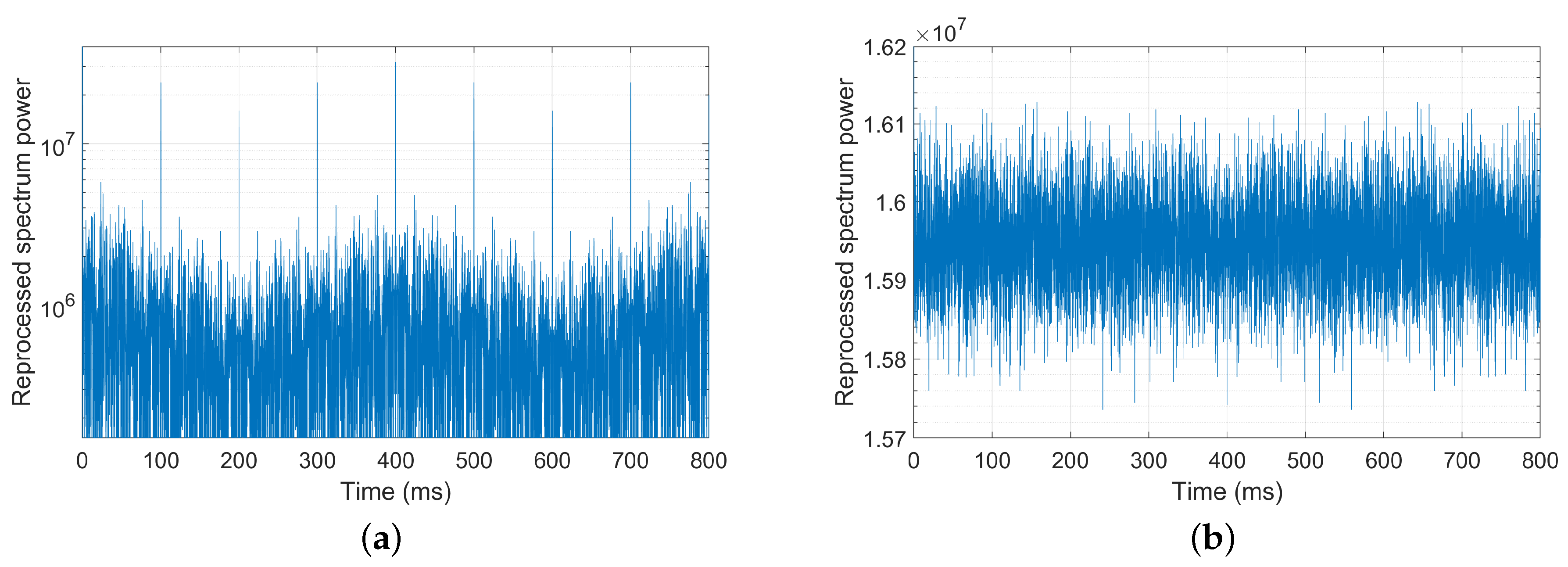
- Noise analysis. Submarine noise is one of the main interferences with the quality of underwater communication. They come from a variety of sources, such as marine life, sea quakes, rain, artificial constructions, etc. The ambient noise of transducers are highly random, and the analysis of their statistical distribution feature helps potentially to improve the reliability of underwater communication modalities.
2. Message Signal Modulation
- (1)
- Initialize the first element of the sequence with a random value, known as “seed” in computer science;
- (2)
- If , repeat the computation with until the constraint is satisfied, otherwise, go to the next step;
- (3)
- If , repeat the computation until the constraint is satisfied, otherwise, go to the next step;
- (4)
- Compute the next element :
- (5)
- If , task completed, otherwise go back to the second step.
3. Signal Demodulation
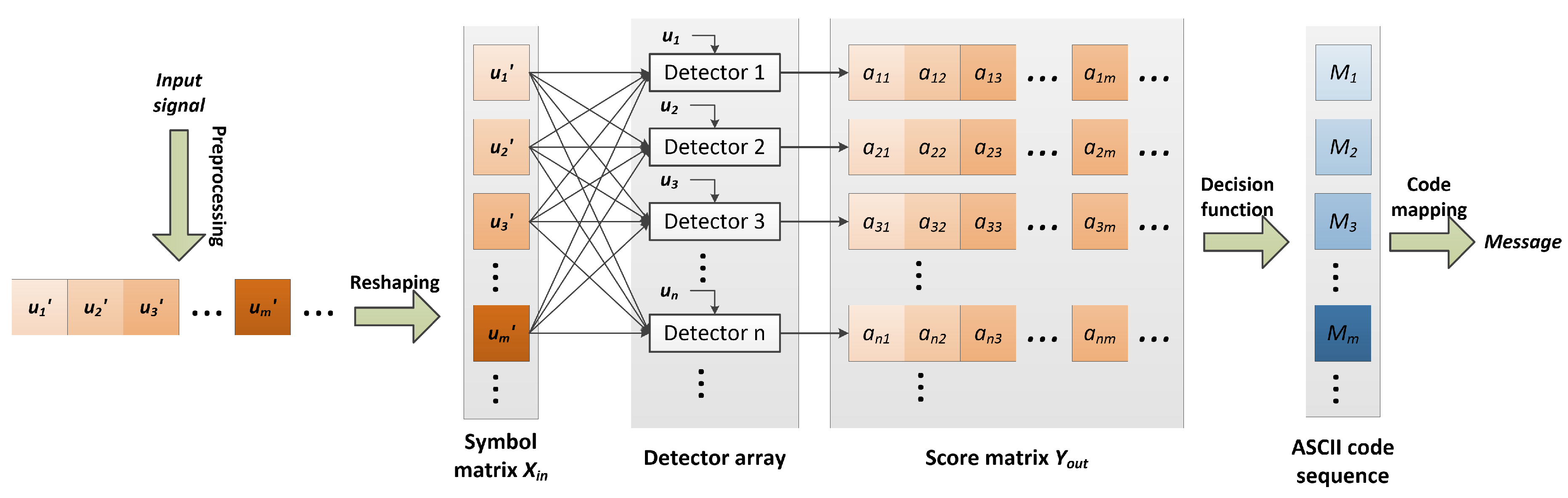
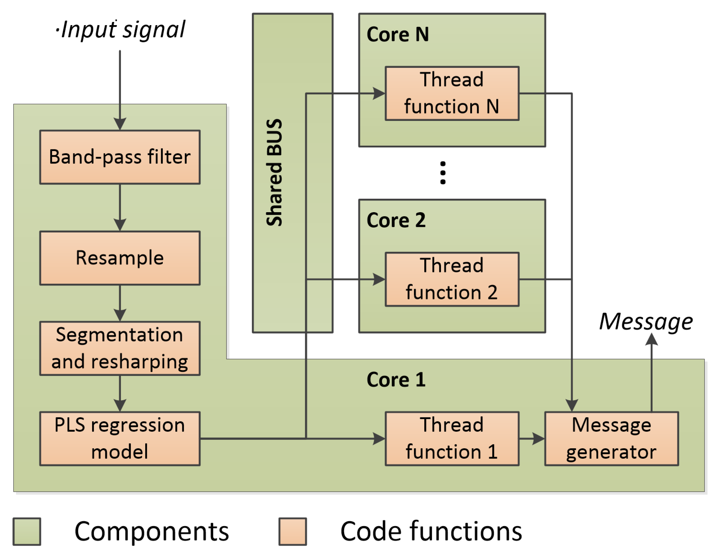
3.1. Architecture of Demodulator
3.2. PLS-Based Detection Method
3.2.1. Training Process of PLS Regression
| Algorithm 1 Pseudocode of PLS Regression Algorithm. |
| Input: training matrix , response variables , projection direction number k Output: regression coefficients
|
3.2.2. Demodulation with PLS Regression
4. Implementation and Optimization
| Algorithm 2 Pseudocode of the Proposed Demodulation Algorithm. |
| Input: input signal , frequency band , normalization coefficients and , regression coefficients , sampling rate , symbol time length T, ASCII table Output: message
|
5. Experiments and Evaluations
5.1. Dataset
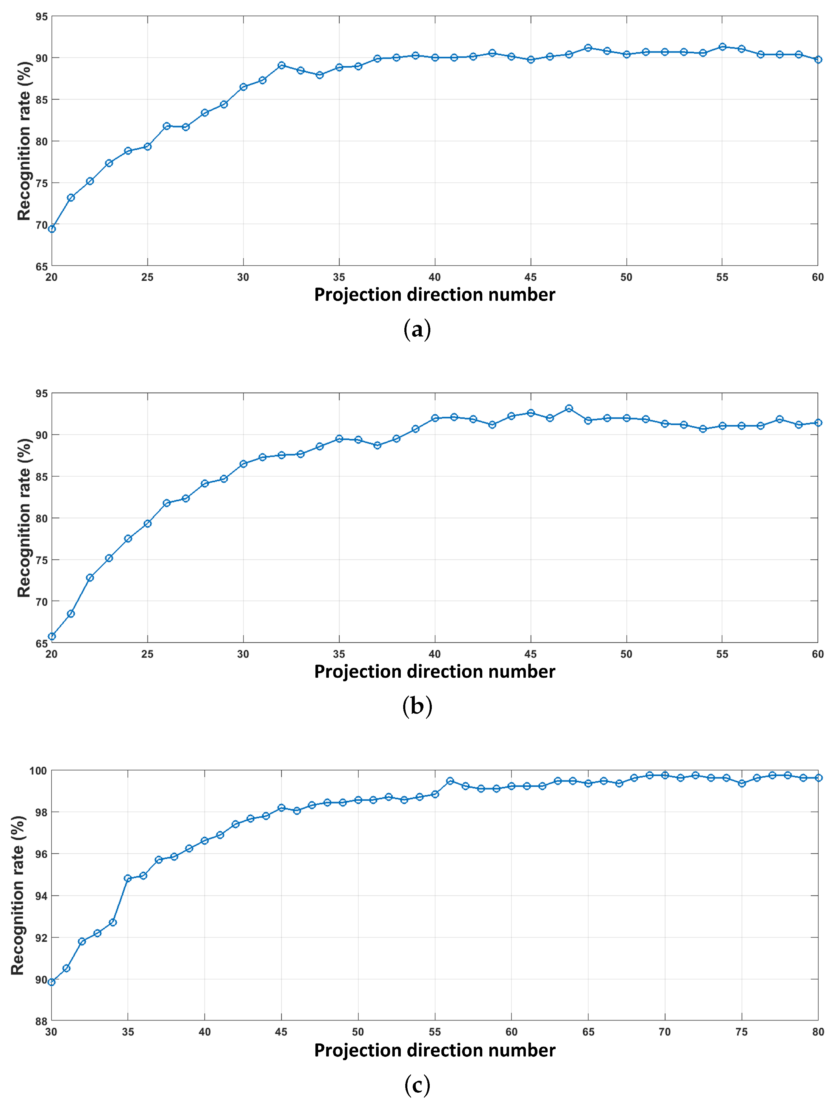
5.2. Parameter Configuration
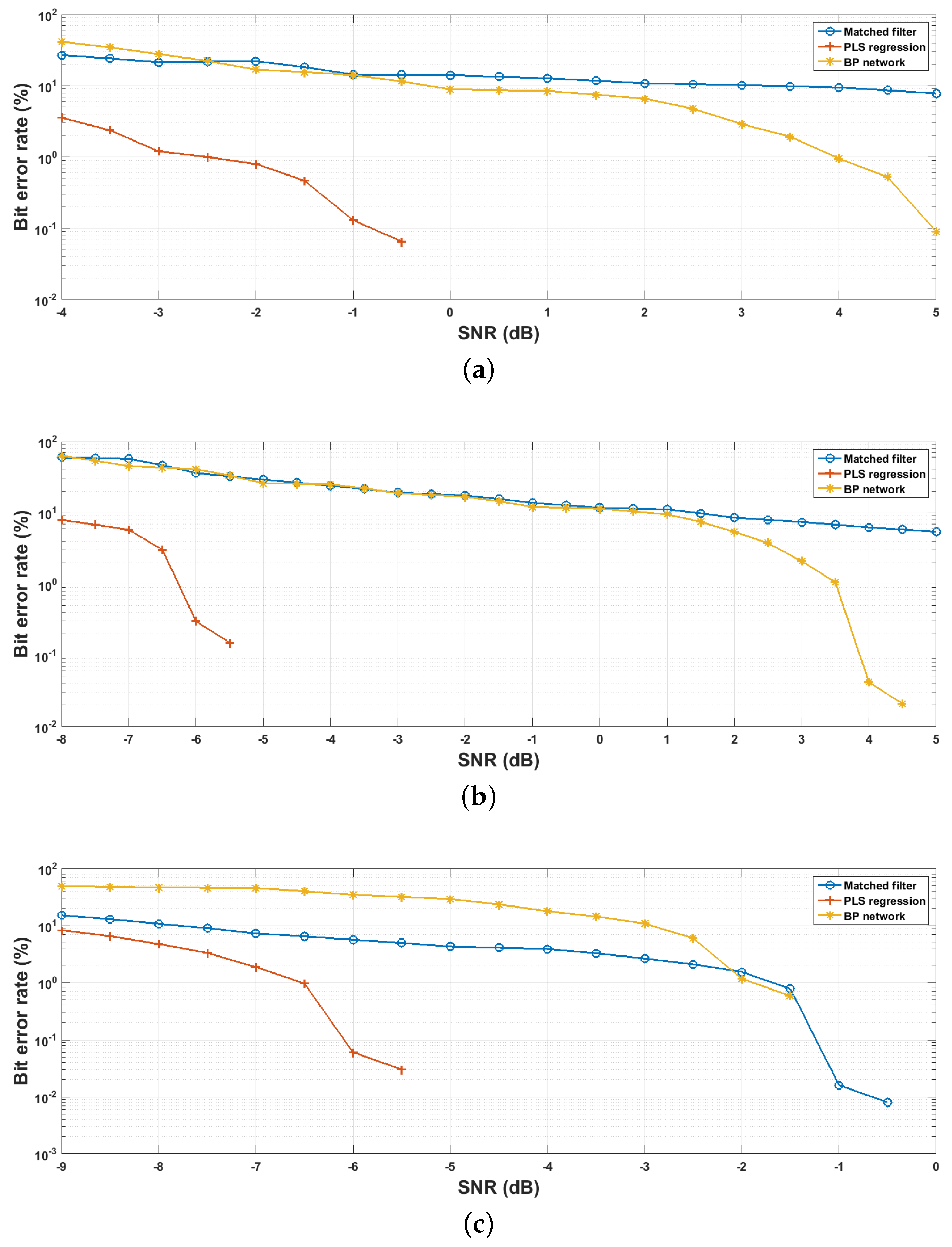
5.3. Demodulation Accuracy Evaluation
5.4. Practicability Analysis
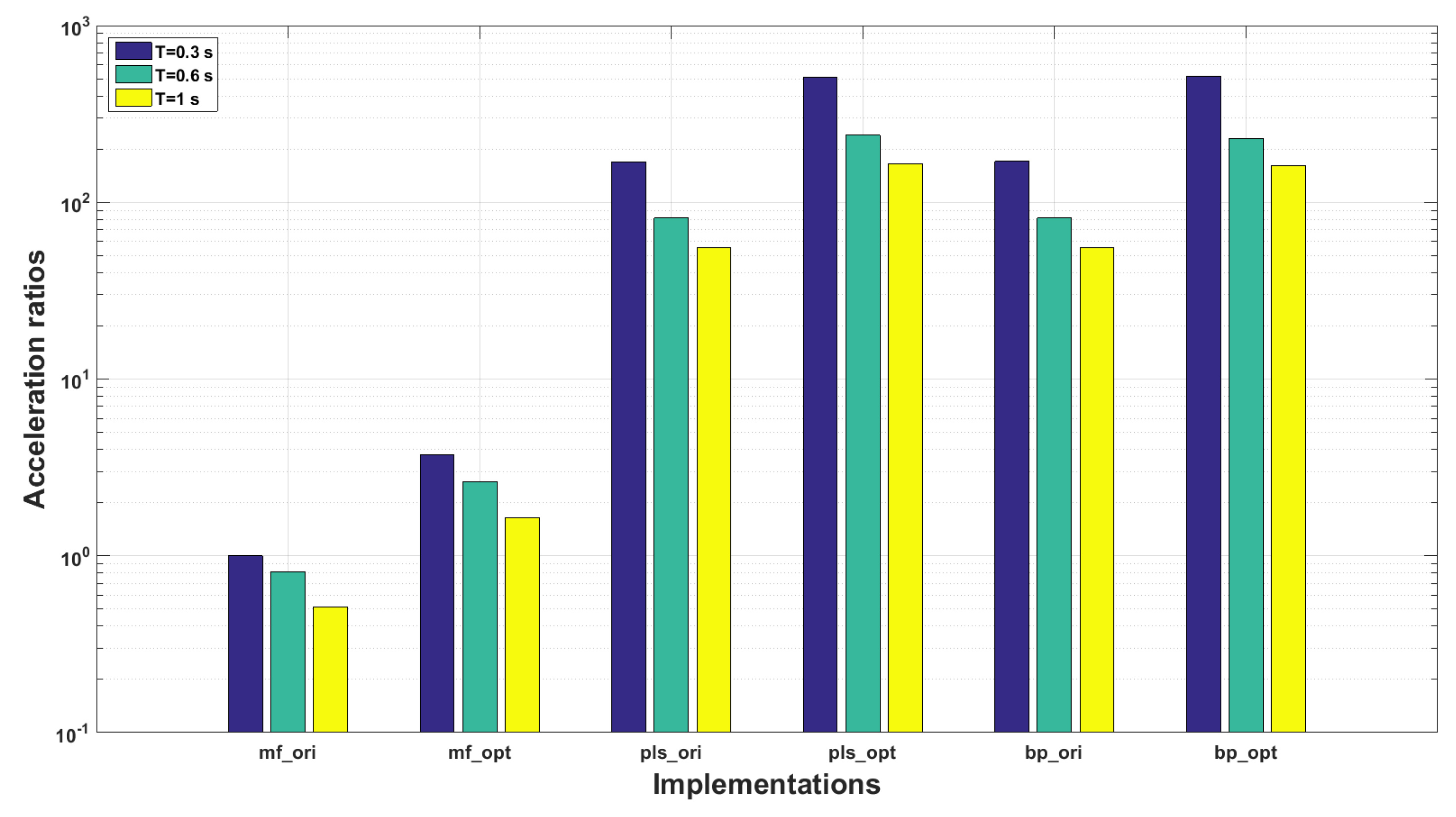
5.5. Temporal Efficiency Evaluation
- a
- the implementations are partly optimized instead of completely parallelized. The multi-thread optimizations of pls_cpu and bp_cpu cover only the message generations without detection steps;
- b
- the shared memory architecture is constrained by the von Nuemann bottle neck, the memory access conflicts may be occurred when multiple thread functions are invoked simultaneously.
6. Conclusions
- -
- The proposed demodulation scheme handles the signal demodulation as a target recognition problem, allowing us to incorporate advanced classification methods into it, benefiting from the recent progresses of pattern recognition techniques. Because machine learning methods are able to statistically analyze the symbol features and noise characters, it can provide better demodulation accuracy performance than matched filters with shorter symbol sequences. That is, if the same accuracy performance is desired, the conventional matched filters need long symbol sequences in order to get enough time gains, so adopting machine learning methods, especially PLS regression, can considerably improve the underwater communication applications in terms of communication rates;
- -
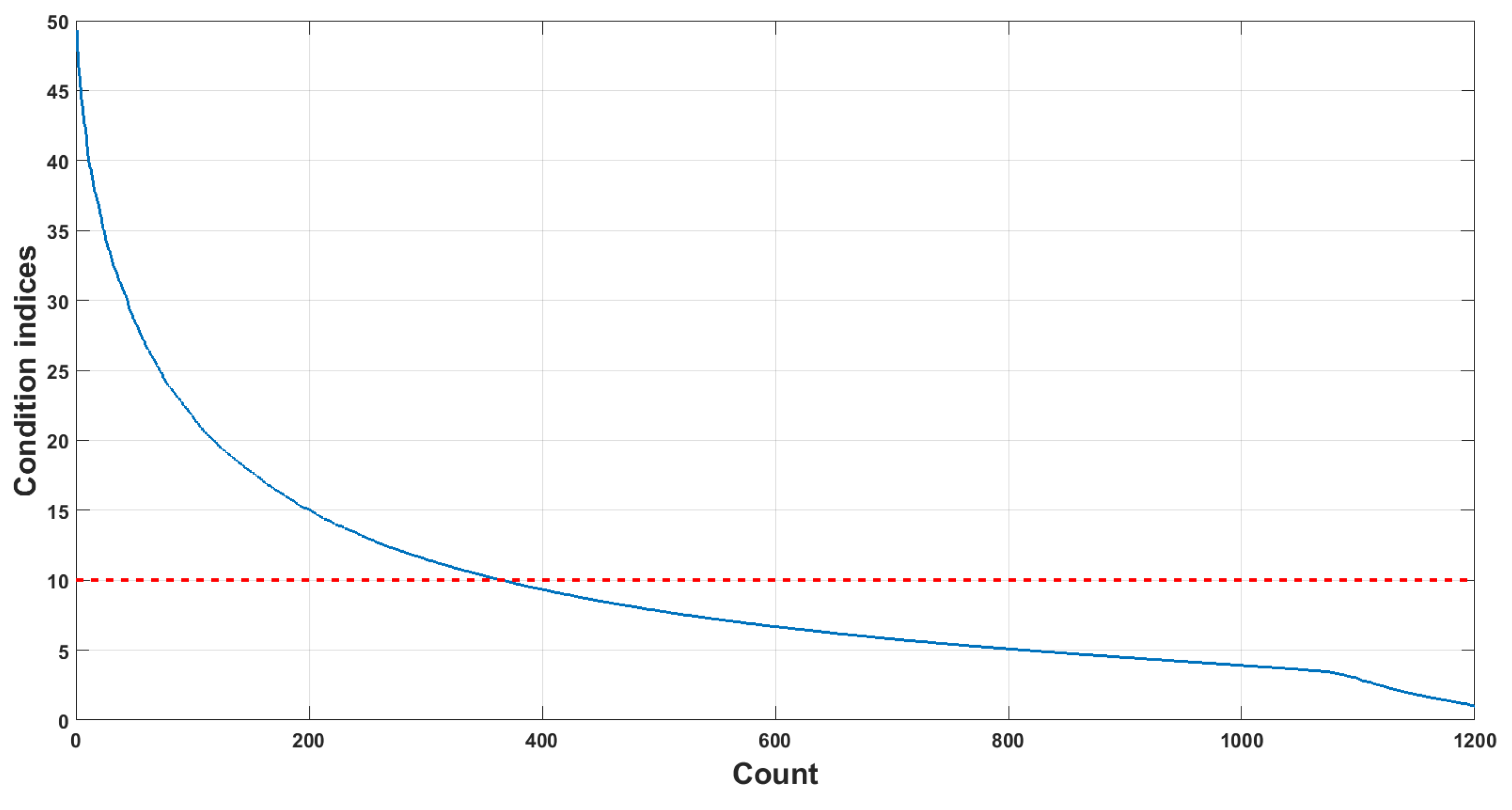
- It is found that the chaos-spreading spectrum signals have the characteristic of multicollinearity which may potentially impact the performance of certain classifiers negatively. Fortunately, the algorithm family of PLS can somehow overcome this disadvantage by modeling the relationships between the predictor and response variables, even with a sparse training dataset;
- -
- The running cost of the proposed approach is very low. The detection steps of the proposed scheme costs only several milliseconds with the experiment protocol of this paper, which even can be ignored during the overall demodulation procedure, so it possesses high temporal efficiency performance;
- -
- The proposed demodulation algorithm can be easily transplanted to other hardware platforms for different purposes. The detection process of the proposed algorithm is actually an operation of matrix production, which can be easily implemented and optimized by using any currently available computing platforms.
Author Contributions
Funding
Conflicts of Interest
References
- Song, H.C. Acoustic communication in deep water exploiting multiple beams with a horizontal array. J. Acoust. Soc. Am. 2012, 132, EL81–EL87. [Google Scholar] [CrossRef] [PubMed]
- Qiao, G.; Babar, Z.; Ma, L.; Liu, S.; Wu, J. MIMO-OFDM underwater acoustic communication systems—A review. Phys. Commun. 2017, 23, 56–64. [Google Scholar] [CrossRef]
- Akyildiz, I.F.; Pompili, D.; Melodia, T. Challenges for efficient communication in underwater acoustic sensor networks. ACM Sigbed Rev. 2004, 1, 3–8. [Google Scholar] [CrossRef]
- Diamant, R.; Lampe, L. Low Probability of Detection for Underwater Acoustic Communication: A Review. IEEE Access 2018, 6, 19099–19112. [Google Scholar] [CrossRef]
- Ganapathy, H.; Pados, D.A.; Karystinos, G.N. New Bounds and Optimal Binary Signature Sets—Part II: Aperiodic Total Squared Correlation. IEEE Trans. Commun. 2011, 59, 1411–1420. [Google Scholar] [CrossRef]
- Sklivanitis, G.; Demirors, E.; Batalama, S.N.; Melodia, T.; Pados, D.A. Receiver configuration and testbed development for underwater cognitive channelization. In Proceedings of the 2014 48th Asilomar Conference on Signals, Systems and Computers, Pacific Grove, CA, USA, 2–5 November 2014; pp. 1594–1598. [Google Scholar]
- Yang, T.C.; Yang, W.B. Low signal-to-noise-ratio underwater acoustic communications using direct-sequence spread-spectrum signals. In Proceedings of the OCEANS 2007—Europe, Aberdeen, UK, 18–21 June 2007; pp. 1–6. [Google Scholar]
- Yang, T.C.; Yang, W.B. Performance analysis of direct-sequence spread-spectrum underwater acoustic communications with low signal-to-noise-ratio input signals. J. Acoust. Soc. Am. 2008, 123, 842–855. [Google Scholar] [CrossRef] [PubMed]
- Rovatti, R.; Setti, G.; Mazzini, G. Chaotic complex spreading sequences for asynchronous DS-CDMA. Part II. Some theoretical performance bounds. IEEE Trans. Circuits Syst. 1998, 45, 496–506. [Google Scholar] [CrossRef]
- Mazzini, G.; Setti, G.; Rovatti, R. Corrections to “Chaotic complex spreading sequences for asynchronous DS-CDMA. I. System modeling and results”. IEEE Trans. Circuits Syst. 1998, 44, 515–516. [Google Scholar] [CrossRef]
- Chen, C.C.; Yao, K.; Umeno, K.; Biglieri, E. Design of spread-spectrum sequences using chaotic dynamical systems and ergodic theory. IEEE Trans. Circuits Syst. 2001, 48, 1110–1114. [Google Scholar] [CrossRef]
- Wang, X.Y.; Zhu, Z.F.; Fang, S.L. Noncooperative detection and parameter estimation of underwater acoustic DSSS-BPSK signal. In Proceedings of the International Conference on Mechatronics and Machine Vision in Practice, Xiamen, China, 4–6 December 2007; pp. 52–56. [Google Scholar]
- Zhang, X. Spread Spectrum Sequence Estimation in Acoustic Non-Cooperative Communication System. In Proceedings of the 2009 International Symposium on Computer Network and Multimedia Technology, Wuhan, China, 18–20 January 2009; pp. 1–4. [Google Scholar]
- Zhang, T.; Dai, S.; Zhang, W.; Ma, G.; Gao, X. Blind estimation of the PN sequence in lower SNR DS-SS signals with residual carrier. Digital Signal Process. 2012, 22, 106–113. [Google Scholar] [CrossRef]
- Zhang, T.; Zhang, W.; Dai, S.; Ma, G.; Jiang, Q. A Spectral Method for Period Detection of PN Sequence for Weak DS-SS Signals in Dynamic Environments. In Proceedings of the 2009 International Conference on Networks Security, Wireless Communications and Trusted Computing, Wuhan, China, 25–26 April 2009; pp. 266–269. [Google Scholar]
- Abel, A.; Schwarz, W. Chaos communications-principles, schemes, and system analysis. Proc. IEEE 2002, 90, 691–710. [Google Scholar] [CrossRef]
- Yang, T. A Survey of Chaotic Secure Communication Systems. Int. J. Comput. Cogn. 2004, 2, 81–130. [Google Scholar]
- Bowong, S.; Kakmeni, F.M.M.; Siewe, M.S. Secure communication via parameter modulation in a class of chaotic systems. Commun. Nonlinear Sci. Numer. Simul. 2007, 12, 397–410. [Google Scholar] [CrossRef]
- Kilfoyle, D.B.; Baggeroer, A.B. The state of the art in underwater acoustic telemetry. IEEE J. Ocean. Eng. 2000, 25, 4–27. [Google Scholar] [CrossRef]
- Kocarev, L.; Jakimoski, G. Logistic map as a block encryption algorithm. Phys. Lett. A 2001, 289, 199–206. [Google Scholar] [CrossRef]
- Yoshida, T.; Mori, H.; Shigematsu, H. Analytic study of chaos of the tent map: Band structures, power spectra, and critical behaviors. J. Stat. Phys. 1983, 31, 279–308. [Google Scholar] [CrossRef]
- Rogers, T.D.; Whitley, D.C. Chaos in the cubic mapping. Math. Model. 1983, 4, 9–25. [Google Scholar] [CrossRef]
- Bayliss, A.; Turkel, E. Mappings and accuracy for Chebyshev pseudo-spectral approximations. J. Comput. Phys. 1992, 101, 349–359. [Google Scholar] [CrossRef]
- Zhang, Z.; Wang, H.; Zhao, Y.; Liu, J.; Yang, L. Frequency modulated radar signal with combined chaotic sequence based on Bernoulli map. J. Commun. Technol. Electron. 2016, 61, 971–979. [Google Scholar] [CrossRef]
- Costa, R.A.D.; Loiola, M.B.; Eisencraft, M. Correlation and spectral properties of chaotic signals generated by a piecewise-linear map with multiple segments. Signal Process. 2016, 133, 187–191. [Google Scholar] [CrossRef]
- Liu, L.; Zhou, S.; Cui, J. Prospects and problems of wireless communication for underwater sensor networks. Wirel. Commun. Mob. Comput. 2008, 8, 977–994. [Google Scholar]
- Turin, G.L. An introduction to matched filters. IRE Trans. Inf. Theory 1960, 6, 311–329. [Google Scholar] [CrossRef]
- Stojanovic, M.; Catipovic, J.A.; Proakis, J.G. Phase-coherent digital communications for underwater acoustic channels. IEEE J. Ocean. Eng. 1994, 19, 100–111. [Google Scholar] [CrossRef]
- Laot, C.; Coince, P. Experimental results on adaptive MMSE turbo equalization in shallow underwater acoustic communication. In Proceedings of the OCEANS’10 IEEE SYDNEY, Sydney, Australia, 24–27 May 2010; pp. 1–5. [Google Scholar]
- Cannelli, L.; Leus, G.; Dol, H.; van Walree, P. Adaptive turbo equalization for underwater acoustic communication. In Proceedings of the 2013 MTS/IEEE OCEANS, Bergen, Norway, 10–14 June 2013; pp. 1–9. [Google Scholar]
- Shimura, T.; Ochi, H.; Watanabe, Y.; Hattori, T. Demonstration of time-reversal communication combined with spread spectrum at the range of 900 km in deep ocean. Acoust. Sci. Technol. 2012, 33, 113–116. [Google Scholar] [CrossRef][Green Version]
- Shu, X.; Wang, H.; Wang, J.; Yang, X. A method of multichannel chaotic phase modulation spread spectrum and its application in underwater acoustic communication. Chin. J. Acoust. 2017, 2, 159–168. [Google Scholar]
- Ushio, T.; Innami, T.; Kodama, S. Chaos Shift Keying Based on In-Phase and Anti-Phase Chaotic Synchronization. IEICE Trans. Fundam. Electron. Commun. Comput. Sci. 1996, 79, 1689–1693. [Google Scholar]
- Yang, J.; Qiu, Z.K.; Li, X.; Zhuang, Z.W. Uncertain chaotic behaviours of chaotic-based frequency- and phase-modulated signals. IET Signal Proc. 2012, 5, 748–756. [Google Scholar] [CrossRef]
- Wang, R.; Guo, J.; Leung, H. Orthogonal Circulant Structure and Chaotic Phase Modulation Based Analog to Information Conversion. Signal Proc. 2017, 144, 104–117. [Google Scholar] [CrossRef]
- Yang, Q.L.; Yan-Fei, L.I.; Zhang, X.Y. The Design of Low Sidelobe and Orthogonal Waveform for MIMO Radar Based on Chaotic Phase-Spectrum Modulation. Electron. Inf. Warfare Technol. 2017. [Google Scholar] [CrossRef]
- Kaddoum, G. Wireless Chaos-Based Communication Systems: A Comprehensive Survey. IEEE Access 2017, 4, 2621–2648. [Google Scholar] [CrossRef]
- Bai, C.; Ren, H.P.; Grebogi, C.; Baptista, M.S. Chaos-Based Underwater Communication With Arbitrary Transducers and Bandwidth. Appl. Sci. 2018, 8, 162. [Google Scholar] [CrossRef]
- Van Nguyen, B.; Jung, H.; Kim, K. On the Anti-Jamming Performance of the NR-DCSK System. Secur. Commun. Netw. 2018, 2018, 7963641. [Google Scholar] [CrossRef]
- Nguyen, D.V.; Rocke, D.M. Tumor classification by partial least squares using microarray gene expression data. Bioinformatics 2002, 18, 39. [Google Scholar] [CrossRef]
- Martens, M.; Martens, H. Partial Least Squares Regression. In Statistical Procedures in Food Research; Elsevier Applied Science: England, UK, 1986; pp. 293–359. [Google Scholar]
- Worsley, K. An overview and some new developments in the statistical analysis of PET and fMRI data. Hum. Brain Map 1997, 5, 254–258. [Google Scholar] [CrossRef]
- Nilsson, J.; Jong, S.D.; Smilde, A.K. Multiway calibration in 3D QSAR. J. Chemom. 1997, 11, 511–524. [Google Scholar] [CrossRef]
- Hulland, J. Use of partial least squares (PLS) in strategic management research: A review of four recent studies. Strat. Manag. J. 1999, 20, 195–204. [Google Scholar] [CrossRef]
- Uzair, M.; Mahmood, A.; Mian, A. Hyperspectral Face Recognition With Spatiospectral Information Fusion and PLS Regression. IEEE Trans. Image Process. 2015, 24, 1127–1137. [Google Scholar] [CrossRef]
- Li, C.; Benezeth, Y.; Nakamura, K.; Gomez, R.; Yang, F. A robust multispectral palmprint matching algorithm and its evaluation for FPGA applications. J. Syst. Archit. 2018, 88, 43–53. [Google Scholar] [CrossRef]
- Li, S.; Mou, X.; Cai, Y. Pseudo-random Bit Generator Based on Couple Chaotic Systems and Its Applications in Stream-Cipher Cryptography. In Proceedings of the International Conference on Cryptology in India, Chennai, India, 16–20 December 2001; pp. 316–329. [Google Scholar]
- Wold, H. Soft Modelling: The Basic Design and Some Extensions. Syst. Indirect Obs. 1982, 36–37. Available online: https://ci.nii.ac.jp/naid/10006132197/en/ (accessed on 28 November 2018).
- Wold, H. Partial least squares. In Encyclopedia of Statistical Sciences; Kotz, S., Johnson, N., Eds.; John Wiley & Sons, Inc.: Hoboken, NJ, USA, 2004. [Google Scholar]
- Wold, S.; Ruhe, A.; Wold, H.; Dunn, W.J., III. The collinearity problem in linear regression. The partial least squares (PLS) approach to generalized inverse. SIAM J. Sci. Stat. Comput. 1984, 5, 735–743. [Google Scholar] [CrossRef]
- Shawe-Taylor, J.; Cristianini, N. Kernel Methods for Pattern Analysis; Cambridge University Press: New York, NY, USA, 2004. [Google Scholar]
- Walree, P.A.V.; Socheleau, F.X.; Otnes, R.; Jenserud, T. The Watermark Benchmark for Underwater Acoustic Modulation Schemes. IEEE J. Ocean. Eng. 2017, 42, 1007–1018. [Google Scholar] [CrossRef]
- Widrow, B.; Mccool, J.M.; Larimore, M.G.; Johnson, C.R. Stationary and Nonstationary Learning Characteristics of the LMS Adaptive Filter; Springer: Cham, Switzerland, 1977; pp. 355–393. [Google Scholar]
- Lu, L.; Zhao, H.; Chen, B. Improved-Variable-Forgetting-Factor Recursive Algorithm Based on the Logarithmic Cost for Volterra System Identification. IEEE Trans. Circuits Syst. Express Briefs 2016, 63, 588–592. [Google Scholar] [CrossRef]
- Li, W.; Preisig, J.C. Estimation of Rapidly Time-Varying Sparse Channels. IEEE J. Ocean. Eng. 2008, 32, 927–939. [Google Scholar] [CrossRef]
- Jin, W.; Li, Z.J.; Wei, L.S.; Zhen, H. The improvements of BP neural network learning algorithm. In Proceedings of the 2000 5th International Conference on Signal Processing Proceedings, Beijing, China, 21–25 August 2000; pp. 1647–1649. [Google Scholar]
- Barons, M.J.; Parsons, N.; Griffiths, F.; Thorogood, M. A comparison of artificial neural network, latent class analysis and logistic regression for determining which patients benefit from a cognitive behavioural approach to treatment for non-specific low back pain. In Proceedings of the 2013 IEEE Symposium on Computational Intelligence in Healthcare and e-health (CICARE), Singapore, 16–19 April 2013; pp. 7–12. [Google Scholar]
- Fildes, R. Conditioning Diagnostics: Collinearity and Weak Data in Regression. Technometrics 1993, 35, 85–86. [Google Scholar]
- David, A.B.; Edwin, K.; Welsch, R.E. Conditioning Diagnostics: Collinearity and Weak Data in Regression; Wiley: Hoboken, NJ, USA, 2005. [Google Scholar]
- Sipser, M. Introduction to the Theory of Computation, 2nd ed.; Thomson Course Technology: Boston, MA, USA, 2005. [Google Scholar]
- Johnson, D.S.; Papadimitriou, C.H. Computational complexity. In Local Search in Combinatorial Optimization; John Wiley and Sons Ltd.: Chichester, UK, 1994; pp. 36–60. [Google Scholar]


| Parameters | Values | Descriptions |
|---|---|---|
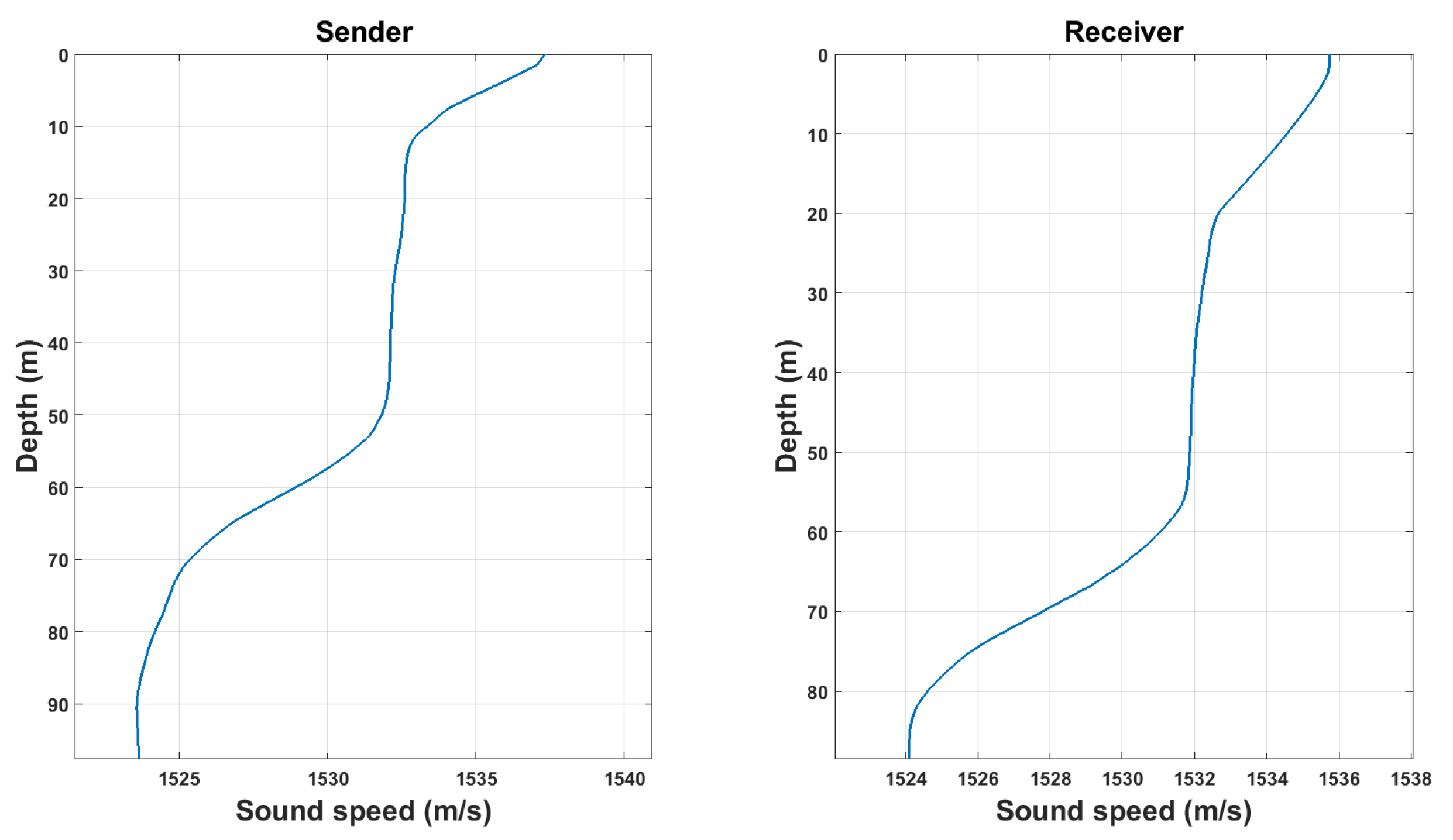
| Sea depth | 90–100 m | Minimum and maximum sea depths during the propagation. |
| Distance | km | Both of the sender and receiver are stationary during the transmission. |
| Source level | 200 dB | - |
| Impulse period | 2 s | - |
| Impulse form | Chaotic | - |
| Sampling rate | 4000 Hz | - |
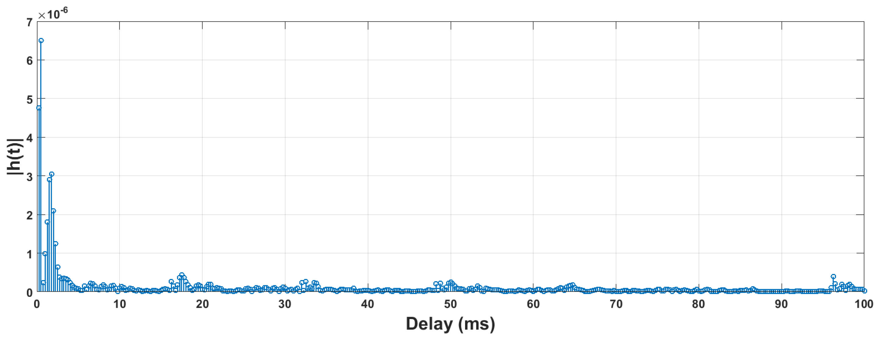
| Channel tap number | 400 | s. |
| Channel estimation interval | 10 ms | - |
| SNR | 0 | ||||||||||||
|---|---|---|---|---|---|---|---|---|---|---|---|---|---|
| BER | |||||||||||||
| SNR | |||||||||||||
| 44.61 | 33.57 | 22.77 | 21.21 | 13.78 | 8.98 | 6.91 | 4.52 | 4.52 | 3.98 | 2.76 | |||
| 30.78 | 25.09 | 10.32 | 9.87 | 6.31 | 5.92 | 3.33 | 2.51 | 0,91 | 0.69 | 0.54 | |||
| 27.14 | 14.12 | 9.75 | 5.01 | 3.82 | 2.01 | 1.21 | 0.82 | 0.51 | 0.42 | 0.21 | |||
| 15.34 | 7.82 | 4.98 | 4.57 | 1.27 | 0.98 | 0.39 | 0.26 | 0.13 | 0.00 | 0.00 | |||
| 10.52 | 4.21 | 2.61 | 1.55 | 0.26 | 0.13 | 0.00 | 0.00 | 0.00 | 0.00 | 0.00 | |||
| 6.45 | 3.13 | 1.27 | 0.52 | 0.26 | 0.13 | 0.00 | 0.00 | 0.00 | 0.00 | 0.00 | |||
| 4.33 | 1.01 | 0.13 | 0.13 | 0.13 | 0.00 | 0.00 | 0.00 | 0.00 | 0.00 | 0.00 | |||
| 3.78 | 0.26 | 0.13 | 0.00 | 0.00 | 0.00 | 0.00 | 0.00 | 0.00 | 0.00 | 0.00 | |||
| 2.21 | 0.51 | 0.00 | 0.00 | 0.00 | 0.00 | 0.00 | 0.00 | 0.00 | 0.00 | 0.00 | |||
| 1.88 | 0.31 | 0.00 | 0.00 | 0.00 | 0.00 | 0.00 | 0.00 | 0.00 | 0.00 | 0.00 | |||
| 0 | 0.91 | 0.26 | 0.00 | 0.00 | 0.00 | 0.00 | 0.00 | 0.00 | 0.00 | 0.00 | 0.00 | ||
| Names | Algorithms | Optimzations |
|---|---|---|
| mf_ori | Matched filter | None |
| mf_opt | Multi-thread parallelization | |
| bp_ori | BP network | None |
| bp_opt | Multi-thread parallelization | |
| pls_ori | PLS regression | None |
| pls_opt | Multi-thread parallelization |
© 2018 by the authors. Licensee MDPI, Basel, Switzerland. This article is an open access article distributed under the terms and conditions of the Creative Commons Attribution (CC BY) license (http://creativecommons.org/licenses/by/4.0/).
Share and Cite
Li, C.; Marzani, F.; Yang, F. Demodulation of Chaos Phase Modulation Spread Spectrum Signals Using Machine Learning Methods and Its Evaluation for Underwater Acoustic Communication. Sensors 2018, 18, 4217. https://doi.org/10.3390/s18124217
Li C, Marzani F, Yang F. Demodulation of Chaos Phase Modulation Spread Spectrum Signals Using Machine Learning Methods and Its Evaluation for Underwater Acoustic Communication. Sensors. 2018; 18(12):4217. https://doi.org/10.3390/s18124217
Chicago/Turabian StyleLi, Chao, Franck Marzani, and Fan Yang. 2018. "Demodulation of Chaos Phase Modulation Spread Spectrum Signals Using Machine Learning Methods and Its Evaluation for Underwater Acoustic Communication" Sensors 18, no. 12: 4217. https://doi.org/10.3390/s18124217
APA StyleLi, C., Marzani, F., & Yang, F. (2018). Demodulation of Chaos Phase Modulation Spread Spectrum Signals Using Machine Learning Methods and Its Evaluation for Underwater Acoustic Communication. Sensors, 18(12), 4217. https://doi.org/10.3390/s18124217