Discrimination Algorithm and Procedure of Snow Depth and Sea Ice Thickness Determination Using Measurements of the Vertical Ice Temperature Profile by the Ice-Tethered Buoys

Abstract
1. Introduction
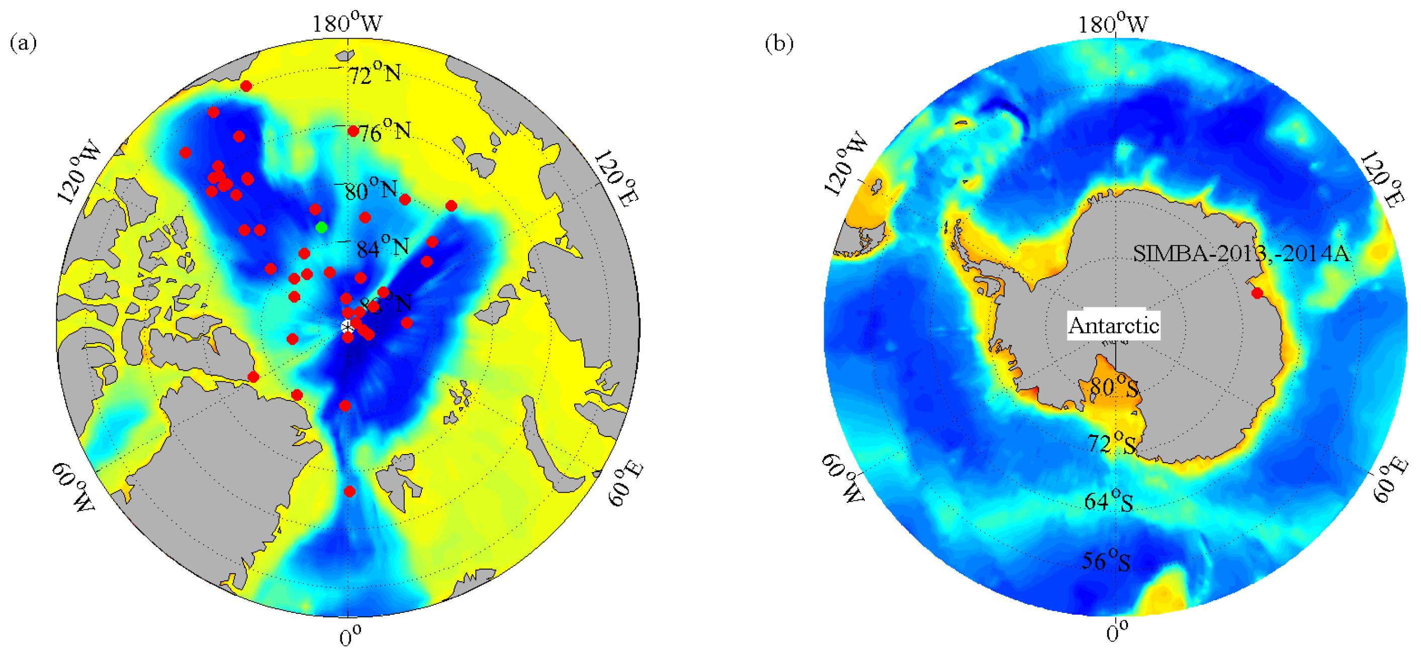
2. Data
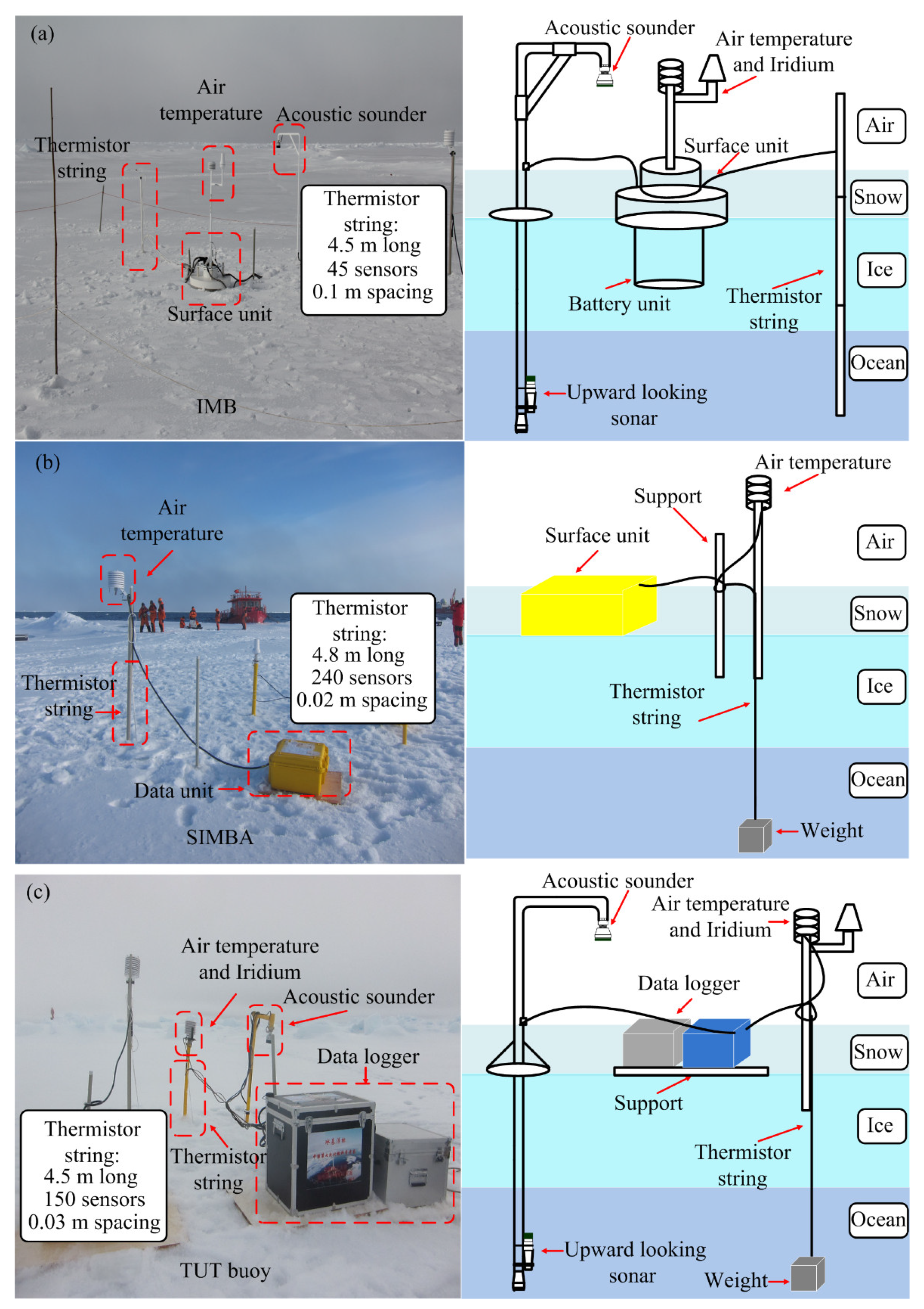
2.1. IMB Data
2.2. SIMBA Data
2.3. TUT Buoy Data
3. Methods for Data Processing
3.1. Determination of the Sea Ice Thickness/Snow Depth and Interfaces Among Air, Snow, Ice, and Water
3.1.1. Interface between Air and Snow or Sea Ice
3.1.2. Interface between Ice and Ocean
3.2. Change Point Detection Method
- Input: The sea ice temperature profile or the daily amplitude of temperature profiles or the vertical temperature gradients Sk (k = 1, 2, 3, …, N).
- Step 1: For the input parameters Sk (k = 1, 2, 3, …, N), we use the Equation (10) to get a change point C0 and two new profiles Sk (k = 1, 2, 3, …, C0) and Sk (k = C0 + 1, C0 + 2, C0 + 3, …, N).
- Step 2: We use the Equation (10) to process Sk (k = 1, 2, 3, …, C0) to get a change point C11. Then a change point C12 detected by the Equation (11) based on Sk (k = C11 + 1, C11 + 2, C11 + 3, …, N). The error of change point estimation is E1.
- Step 3: For the profile Sk (k = C0 + 1, C0 + 2, C0 + 3, …, N), we use the Equation (11) to get a change point C22. A new change point C21 detected by the Equation (10) based on Sk (k = 1, 2, 3, …, C22). The error of change point estimation is E2.
- Step 4: If E1 < E2, C11 and C12 are two change points representing the top and lower interfaces. Otherwise, C21 and C22 are two change points.
- Output: Two change points and calculated ice thickness and snow depth.
3.3. Maximum Likelihood Detection Method
4. Estimation Error
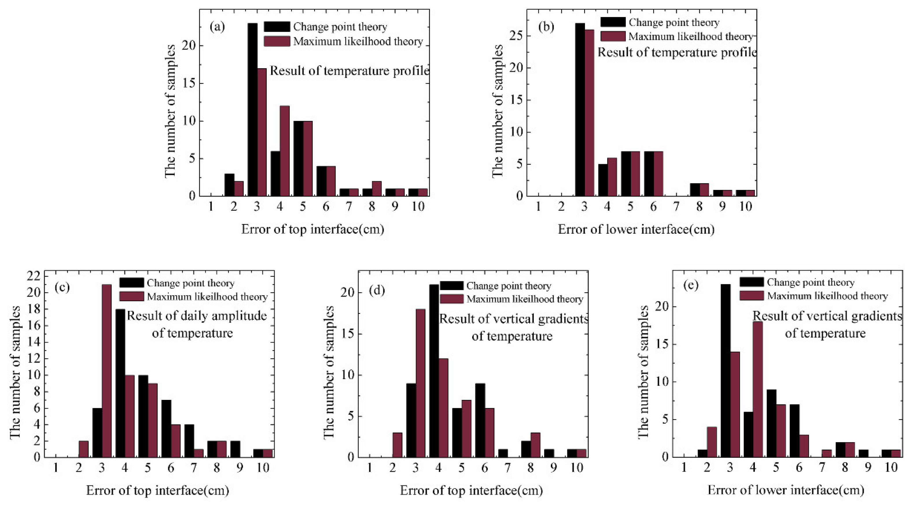
4.1. Estimation Error of the Change Point Detection Method
4.1.1. The Results Calculated Using Ice Temperature Profile
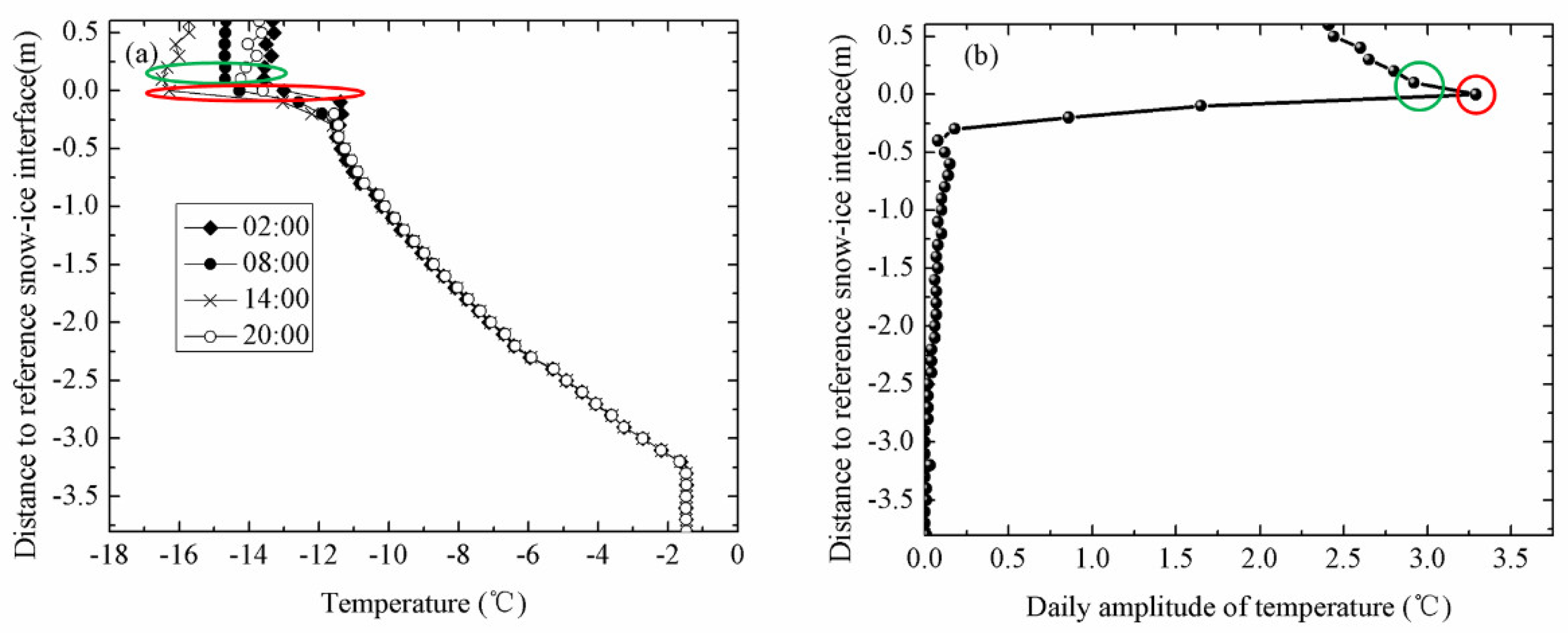
4.1.2. The Results Calculated Using Daily Amplitude of Temperature Profiles
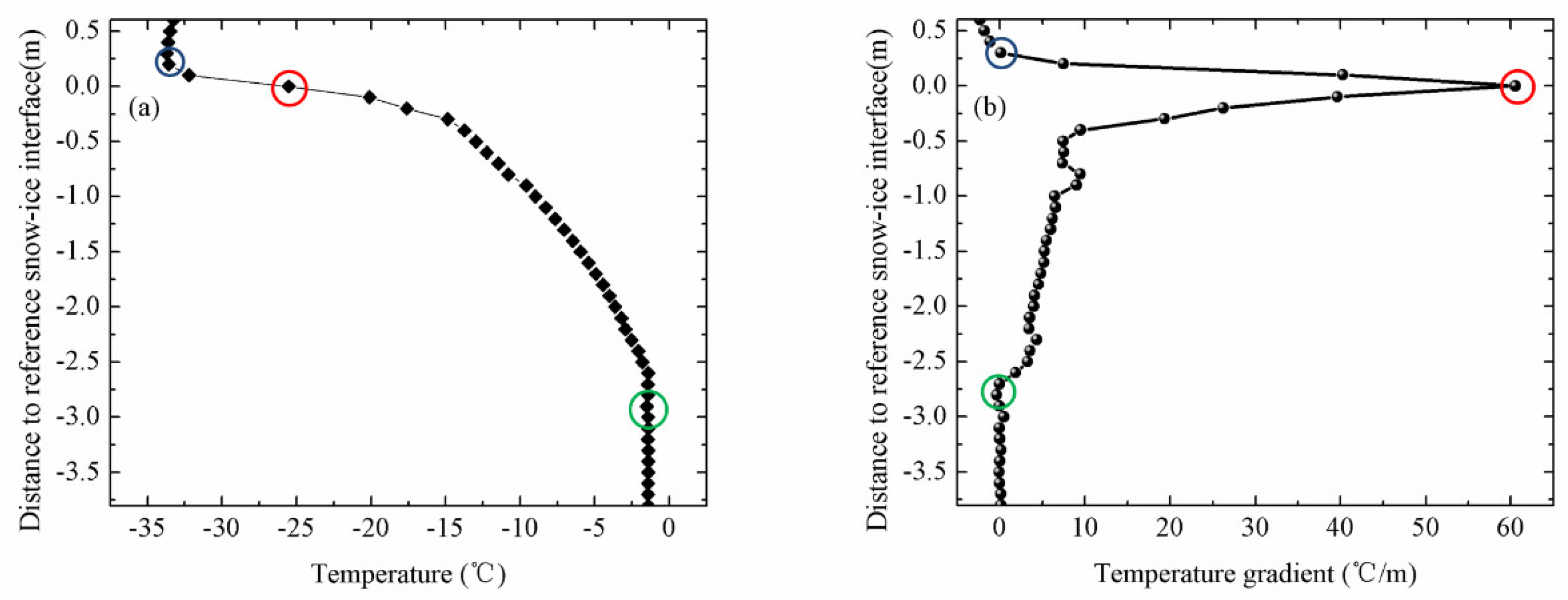
4.1.3. The Results Calculated Using Vertical Gradients of Temperature
4.2. Estimation Error of the Maximum Likelihood Detection Method
4.2.1. The Results Calculated Using Ice Temperature Profile
4.2.2. The Results Calculated Using Daily Amplitude of Temperature Profile
4.2.3. The Results Calculated Using Vertical Gradients of Temperature
4.3. Statistical Errors of the Two Methods
5. Factors Influencing on the Estimation Error
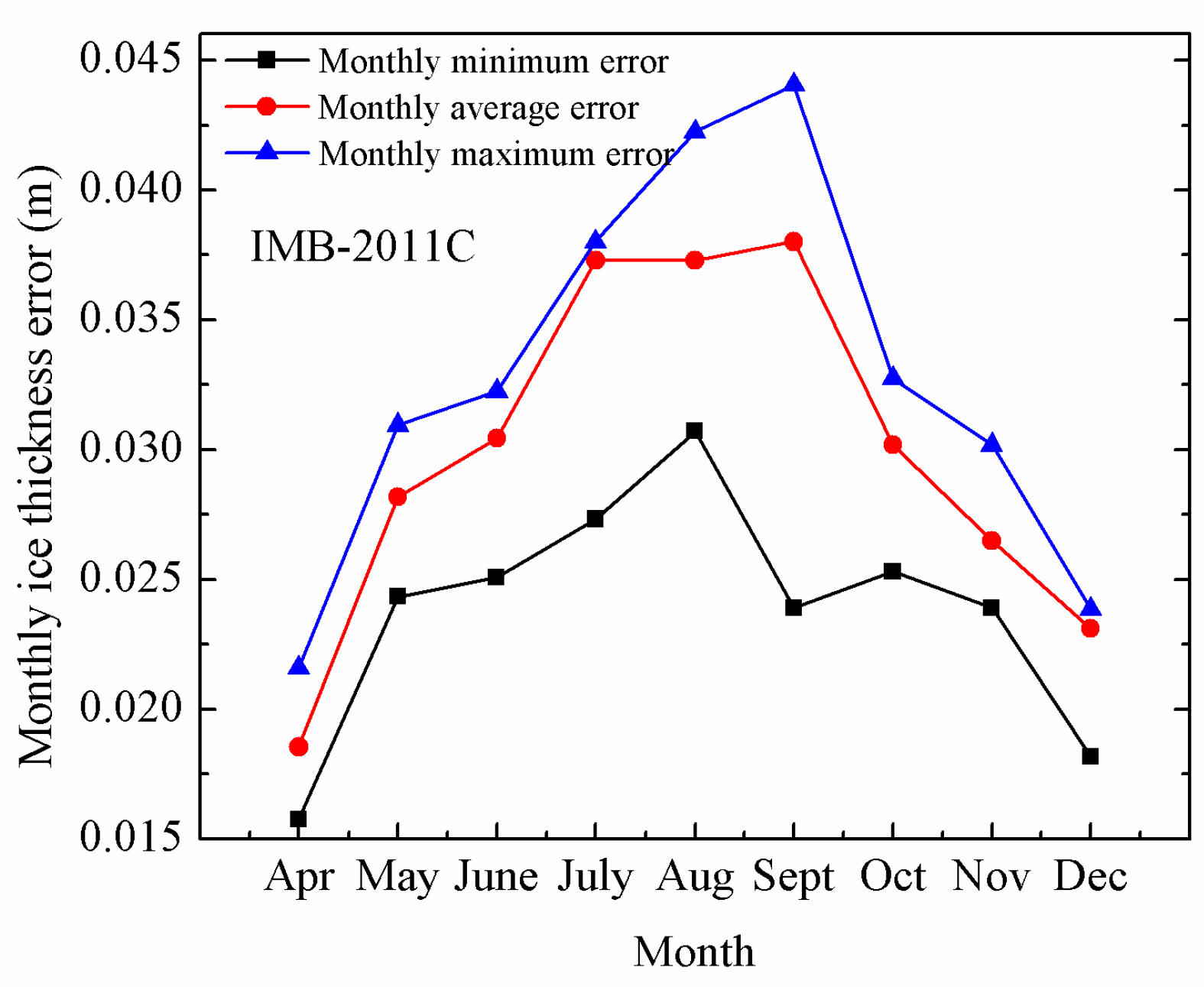
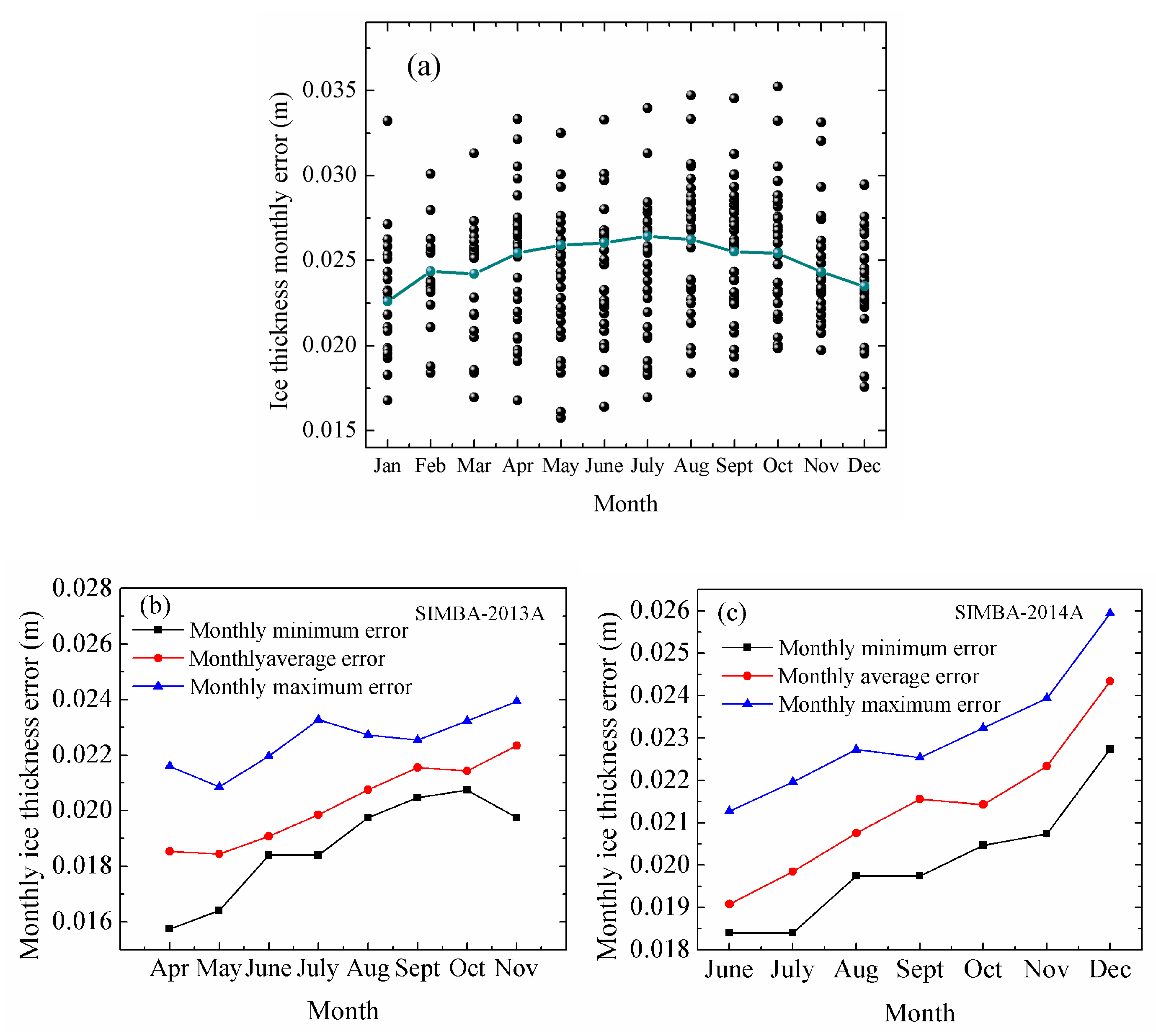
5.1. Seasonal Dependence of Estimation Error
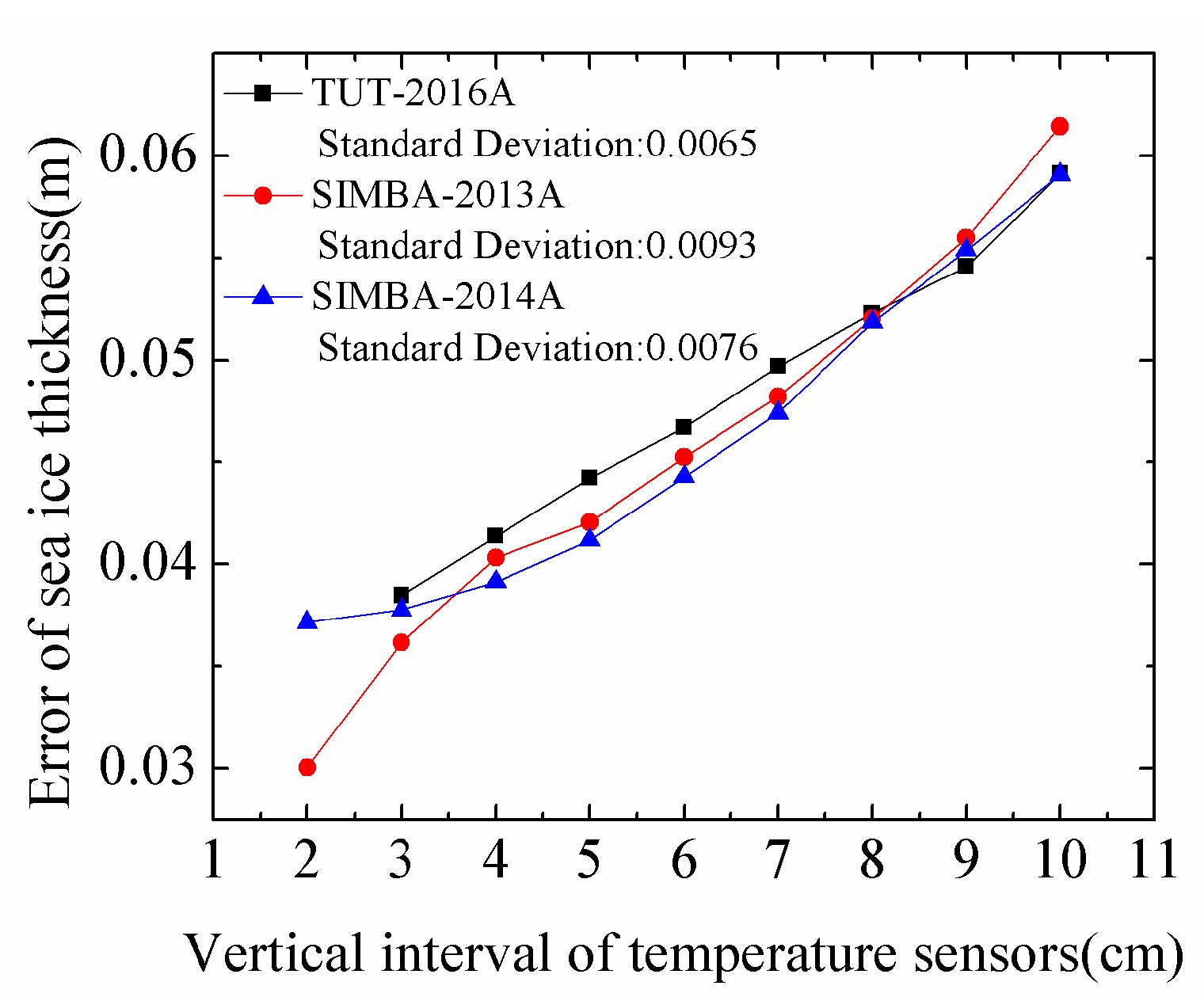
5.2. The Influence of the Vertical Interval of Temperature Sensors
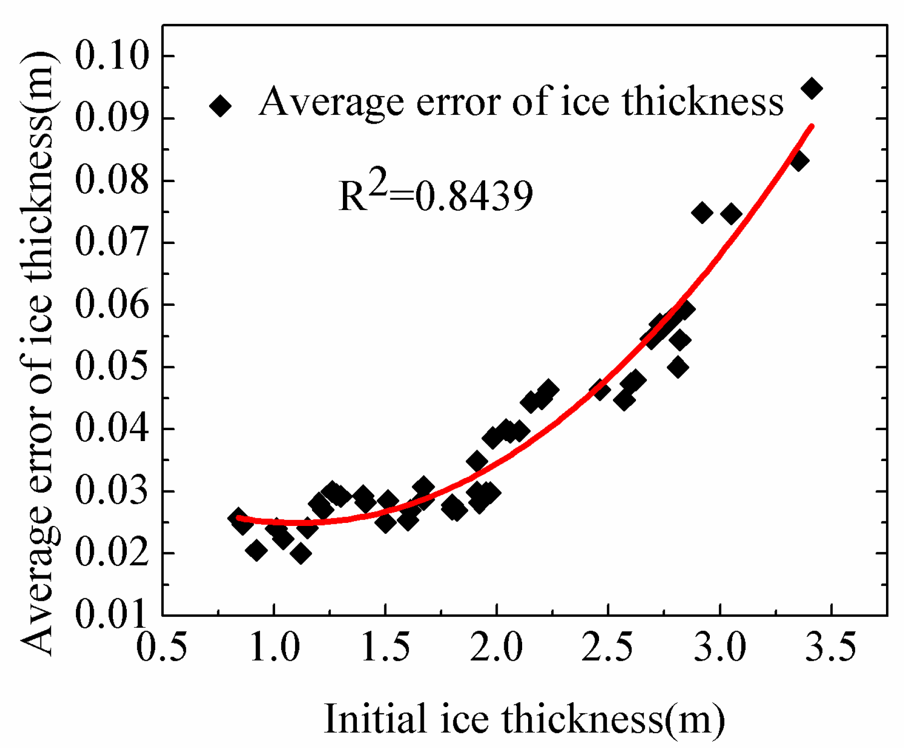
5.3. The Influence of Initial Ice Thickness
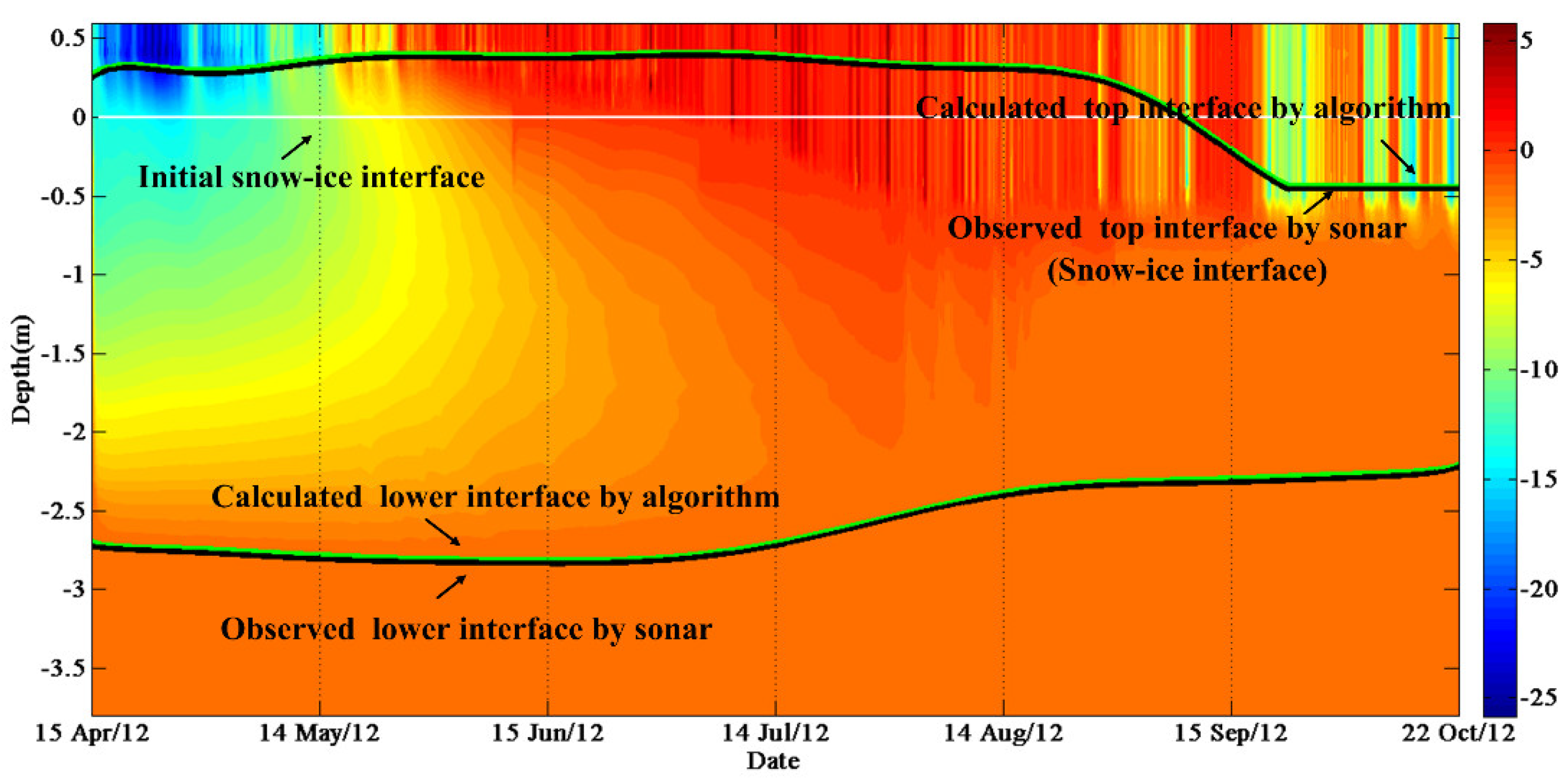
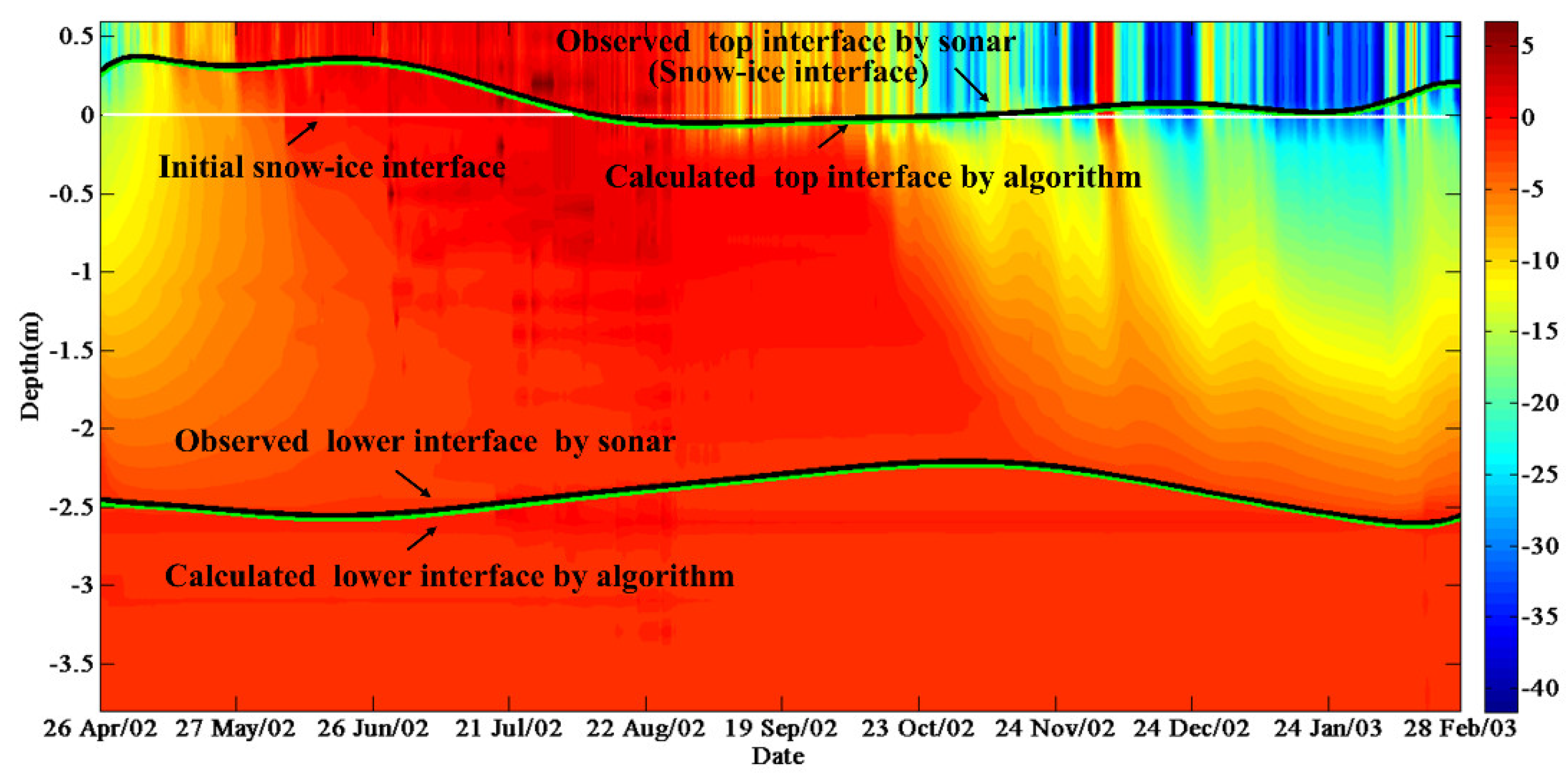
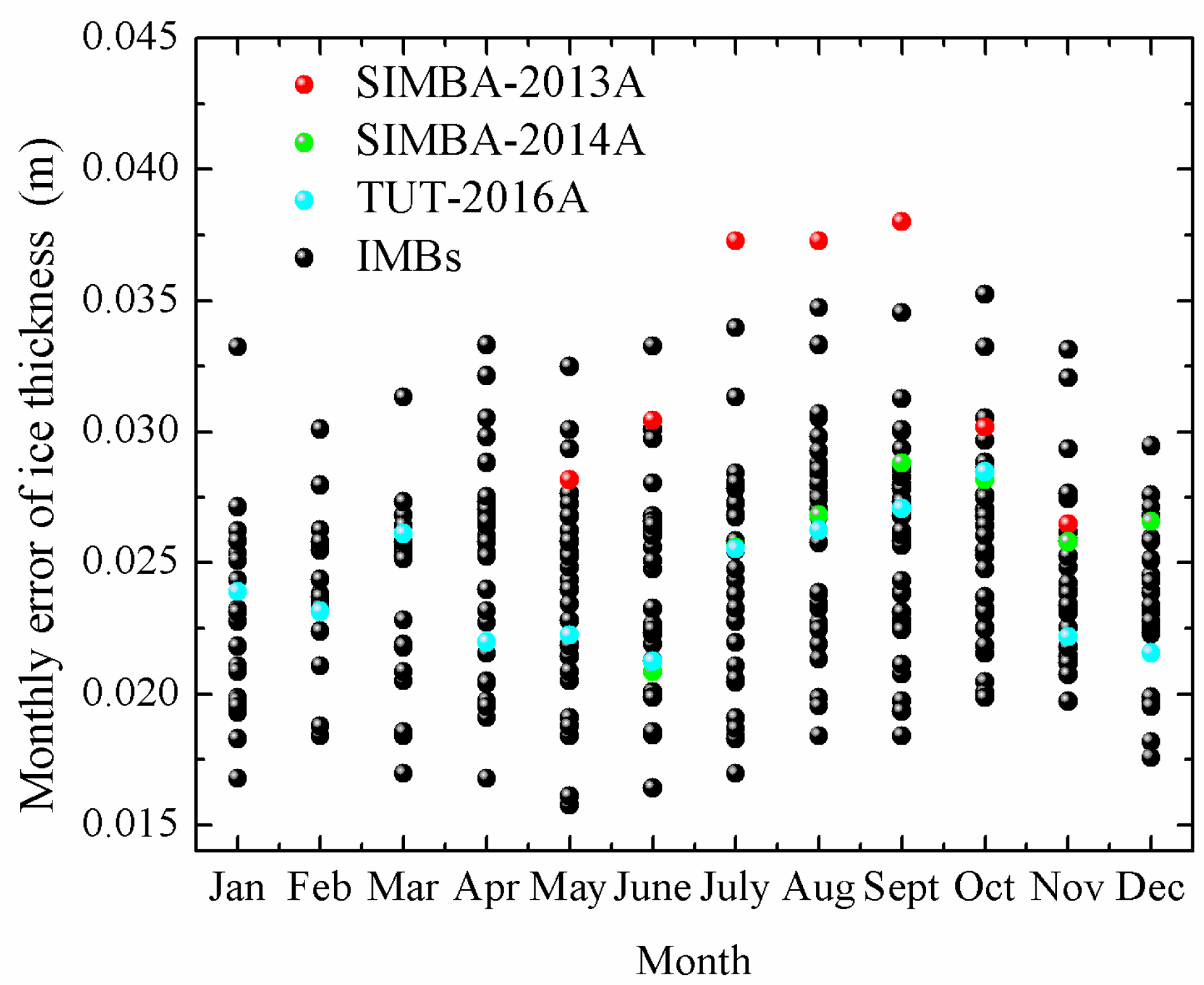
5.4. Comparison between the Results Observed by the Buoys
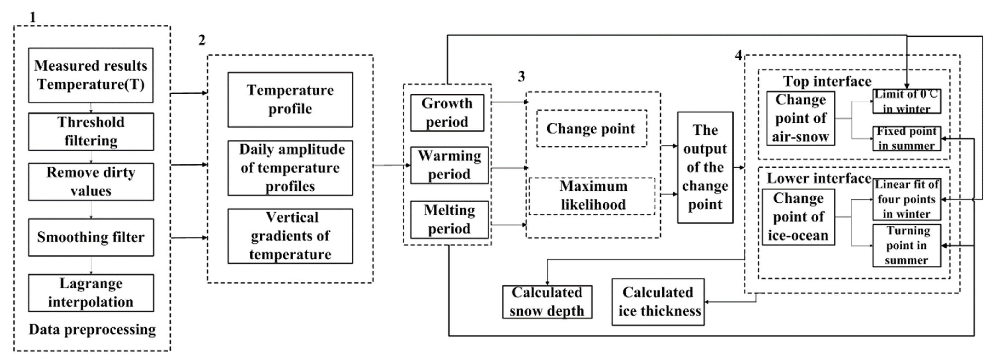
6. Procedure to Determine Snow Depth and Ice Thickness
- Data preprocessing. Firstly, measured results of temperature profile of sea ice are processed by threshold filtering and removing the outliers, such as 30 °C or −60 °C. In the second place, smoothing filter is used to filter out irrelevant data. In the third place, we use interpolation to handle missing values by creating an interpolation function to replace the null values of the temperature profile of sea ice.
- Based on the temperature profiles, the vertical gradients of temperature profiles are calculated. Then the period of sea ice is determined.
- (1)
- Calculate the intersection of the temperature profile and 0 °C. If the intersection is lower than the initial snow-ice interface, the period of sea ice is the melting period.
- (2)
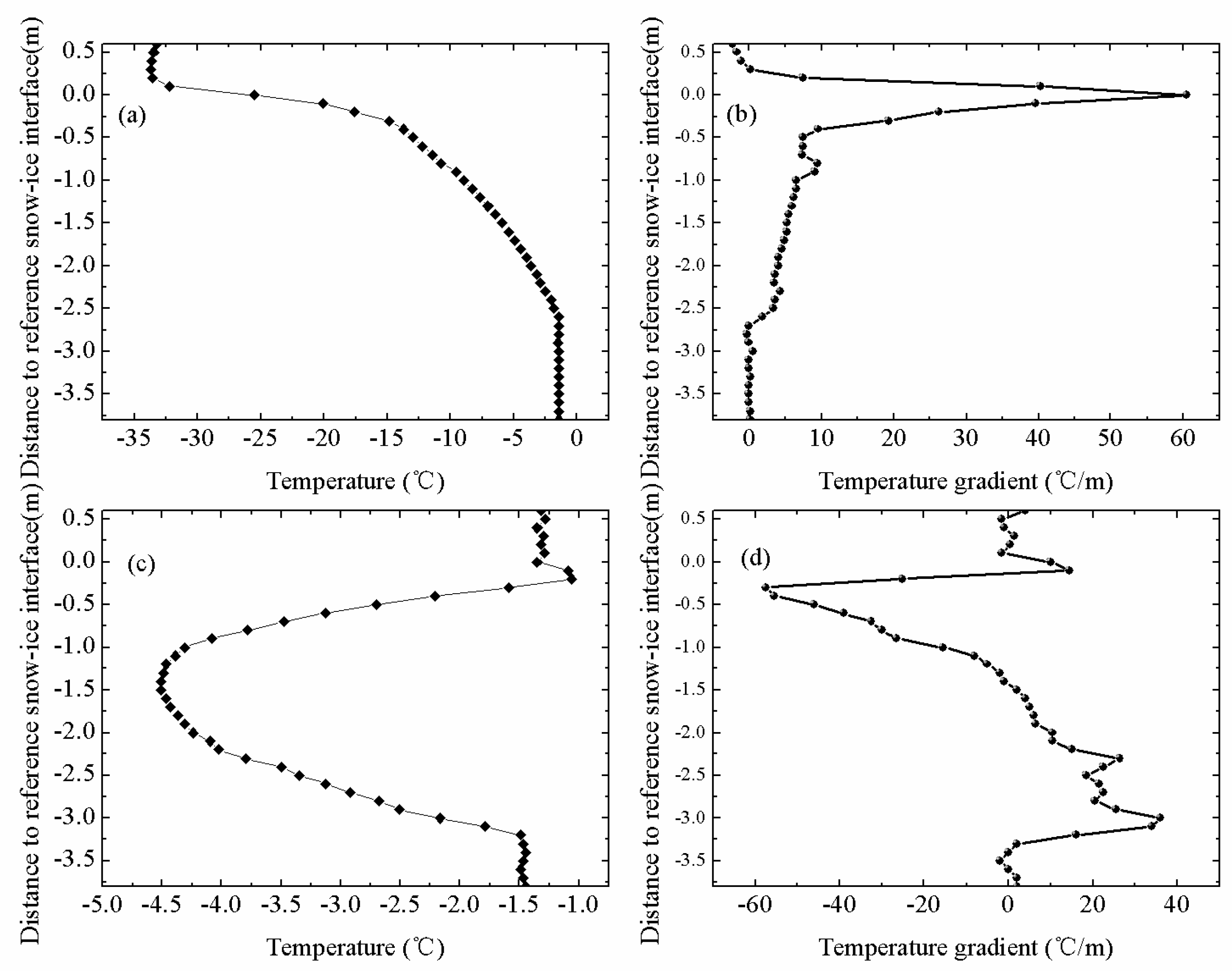
- If the intersection is higher than the initial snow-ice interface, the temperature profiles and the vertical gradients of temperature profiles are used to identify the period of sea ice. If the vertical temperature profile is linear, it is the ice growth period. If the temperature profile is C-type, it is the warming period. And in the growth and warming period, the vertical gradients of temperature profiles are different, thus the period can be identified as shown in Figure 15.
- Use the change point theory and maximum likelihood theory to generate the output of the change points.
- Use the change points to obtain the top and lower interfaces as described in Section 3.1. The snow depths and ice thicknesses are then obtained.
7. Conclusions
Author Contributions
Funding
Acknowledgments
Conflicts of Interest
References
- Screen, J.A.; Simmonds, I. The central role of diminishing sea ice in recent Arctic temperature amplification. Nature 2010, 464, 1334–1337. [Google Scholar] [CrossRef] [PubMed]
- Rothrock, D.A.; Percival, D.B.; Wensnahan, M. The decline in arctic sea-ice thickness: Separating the spatial, annual, and interannual variability in a quarter century of submarine data. J. Geophys. Res. Oceans 2008, 113, C05003. [Google Scholar] [CrossRef]
- Perovich, D.K.; Grenfell, T.C.; Light, B. Transpolar observations of the morphological properties of Arctic sea ice. J. Geophys. Res. 2009, 114, C00A04. [Google Scholar] [CrossRef]
- Frey, K.E.; Perovich, D.K.; Light, B. The spatial distribution of solar radiation under a melting Arctic sea ice cover. Geophys. Res. Lett. 2011, 38, L22501. [Google Scholar] [CrossRef]
- Haas, C.; Thomas, D.N.; Bareiss, J. Surface properties and processes of perennial Antarctic sea ice in summer. J. Glaciol. 2001, 47, 613–625. [Google Scholar] [CrossRef]
- Light, B.; Grenfell, T.C.; Perovich, D.K. Transmission and absorption of solar radiation by Arctic sea ice during the melt season. J. Geophys. Res. 2008, 113, C03023. [Google Scholar] [CrossRef]
- Lei, R.B.; Li, Z.J.; Cheng, Y.F. A new apparatus for monitoring sea ice thickness based on the magnetostrictive–delay–line principle. J. Atmos. Ocean. Technol. 2009, 26, 818–827. [Google Scholar] [CrossRef]
- Laxon, S.; Peacock, N.; Smith, D. High interannual variability of sea ice thickness in the Arctic region. Nature 2003, 425, 947–950. [Google Scholar] [CrossRef] [PubMed]
- Liu, J.; Schmidt, G.A.; Martinson, D.G. Sensitivity of sea ice to physical parameterizations in the GISS global climate model. J. Geophys. Res. 2003, 108, 3053. [Google Scholar] [CrossRef]
- Kwok, R.; Rothrock, D.A. Decline in Arctic sea ice thickness from submarine and ICESat records: 1958–2008. Geophys. Res. Lett. 2009, 36. [Google Scholar] [CrossRef]
- Haas, C.; Hendricks, S.; Eicken, H. Synoptic airborne thickness surveys reveal state of Arctic sea ice cover. Geophys. Res. Lett. 2010, 37. [Google Scholar] [CrossRef]
- Haas, C.; Pfaffling, A.; Hendricks, S. Reduced ice thickness in Arctic Transpolar Drift favours rapid ice retreat. Geophys. Res. Lett. 2008, 35, L17501. [Google Scholar] [CrossRef]
- Rack, W.; Haas, C.; Langhorne, P. Airborne thickness and freeboard measurements over the McMurdo Ice Shelf, Antarctica, and implications for ice density. J. Geophys. Res. Oceans 2013, 118, 5899–5907. [Google Scholar] [CrossRef]
- Perovich, D.K.; Elder, B. Estimates of ocean heat flux at SHEBA. Geophys. Res. Lett. 2002, 29, 1344. [Google Scholar] [CrossRef]
- Lei, R.B.; Li, N.; Heil, P. Multiyear sea ice thermal regimes and oceanic heat flux derived from an ice mass balance buoy in the Arctic Ocean. J. Geophys. Res. Oceans 2014, 119, 537–547. [Google Scholar] [CrossRef]
- Lei, R.B.; Cheng, B.; Heil, P. Seasonal and Interannual Variations of Sea Ice Mass Balance from the Central Arctic to the Greenland Sea. J. Geophys. Res. Oceans 2018, 123, 2422–2439. [Google Scholar] [CrossRef]
- Richter-Menge, J.A.; Perovich, D.K.; Elder, B. Ice mass balance buoys: A tool for measuring and attributing changes in the thickness of the Arctic sea ice cover. Ann. Glaciol. 2006, 44, 205–210. [Google Scholar] [CrossRef]
- Jackson, K.; Wilkinson, J.; Maksym, T. A novel and low cost sea ice mass balance buoy. J. Atmos. Ocean. Technol. 2013, 30, 13825. [Google Scholar] [CrossRef]
- McPhee, M.G.; Untersteiner, N. Using sea ice to measure heat flux in the ocean. J. Geophys. Res. Oceans 1982, 87, 2071–2074. [Google Scholar] [CrossRef]
- Cheng, B.; Zhang, Z.H.; Vihma, T. Model experiments on snow and ice thermodynamics in the Arctic Ocean with CHINARE 2003 data. J. Geophys. Res. 2008, 113, C09020. [Google Scholar] [CrossRef]
- Hoppmann, M.; Nicolaus, M.; Hunkeler, P.A. Seasonal evolution of an ice-shelf influenced fast-ice regime, derived from an autonomous thermistor chain. J. Geophys. Res. Oceans 2015, 120, 1703–1724. [Google Scholar] [CrossRef]
- Provost, C.; Sennéchael, N.; Miguet, J. Observations of flooding and snow-ice formation in a thinner Arctic sea ice regime during the N-ICE2015 campaign: Influence of basal ice melt and storms. J. Geophys. Res. Oceans 2017, 122, 7115–7134. [Google Scholar] [CrossRef]


| Buoy Type | Interval of Temperature Sensor/m | Length of Thermistor String/m | Buoy Number | Sonar 1 | Temperature Accuracy/°C |
|---|---|---|---|---|---|
| IMB | 0.10 | 4.5 | 47 | Y | ±0.1 |
| SIMBA | 0.02 | 4.8 | 2 | N | ±0.1 |
| TUT | 0.03 | 4.5 | 1 | Y | ±0.1 |
| Method | Parameter | Error of Snow Depth/m | Error of Ice Thickness/m |
|---|---|---|---|
| Change point method | Temperature profile | 0.036 ± 0.016 | 0.039 ± 0.017 |
| Change point method | Daily amplitude of temperature | 0.046 ± 0.016 | |
| Change point method | Vertical gradients of temperature | 0.046 ± 0.016 | 0.038 ± 0.017 |
| Maximum likelihood method | Temperature profile | 0.038 ± 0.015 | 0.036 ± 0.017 |
| Maximum likelihood method | Daily amplitude of temperature | 0.037 ± 0.016 | |
| Maximum likelihood method | Vertical gradients of temperature | 0.038 ± 0.016 | 0.037 ± 0.016 |
© 2018 by the authors. Licensee MDPI, Basel, Switzerland. This article is an open access article distributed under the terms and conditions of the Creative Commons Attribution (CC BY) license (http://creativecommons.org/licenses/by/4.0/).
Share and Cite
Zuo, G.; Dou, Y.; Lei, R. Discrimination Algorithm and Procedure of Snow Depth and Sea Ice Thickness Determination Using Measurements of the Vertical Ice Temperature Profile by the Ice-Tethered Buoys. Sensors 2018, 18, 4162. https://doi.org/10.3390/s18124162
Zuo G, Dou Y, Lei R. Discrimination Algorithm and Procedure of Snow Depth and Sea Ice Thickness Determination Using Measurements of the Vertical Ice Temperature Profile by the Ice-Tethered Buoys. Sensors. 2018; 18(12):4162. https://doi.org/10.3390/s18124162
Chicago/Turabian StyleZuo, Guangyu, Yinke Dou, and Ruibo Lei. 2018. "Discrimination Algorithm and Procedure of Snow Depth and Sea Ice Thickness Determination Using Measurements of the Vertical Ice Temperature Profile by the Ice-Tethered Buoys" Sensors 18, no. 12: 4162. https://doi.org/10.3390/s18124162
APA StyleZuo, G., Dou, Y., & Lei, R. (2018). Discrimination Algorithm and Procedure of Snow Depth and Sea Ice Thickness Determination Using Measurements of the Vertical Ice Temperature Profile by the Ice-Tethered Buoys. Sensors, 18(12), 4162. https://doi.org/10.3390/s18124162