A Low-Light Sensor Image Enhancement Algorithm Based on HSI Color Model


Abstract
1. Introduction
2. Related Works
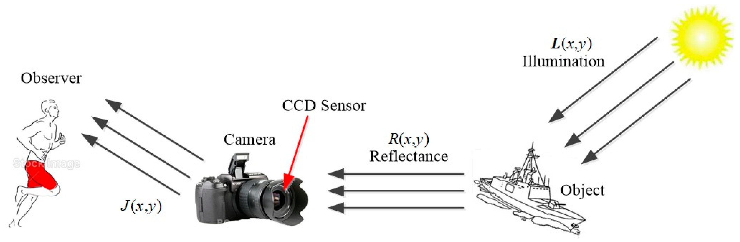
2.1. Retinex Model
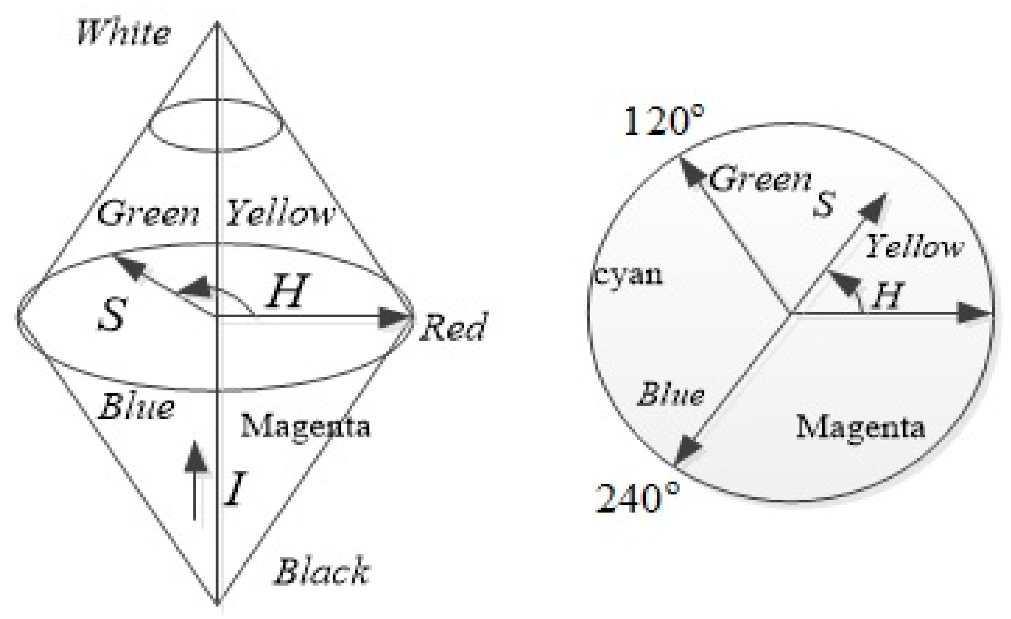
2.2. HSI Color Model
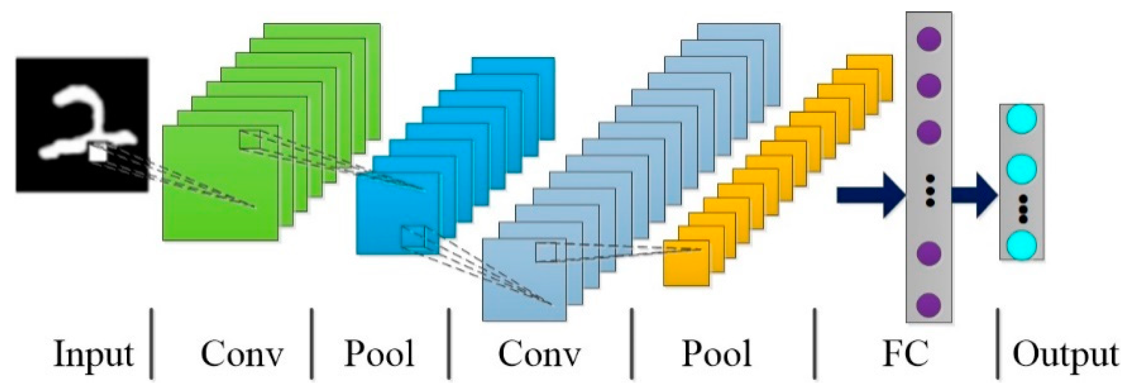
2.3. Convolutional Neural Network Model
3. Proposed Method
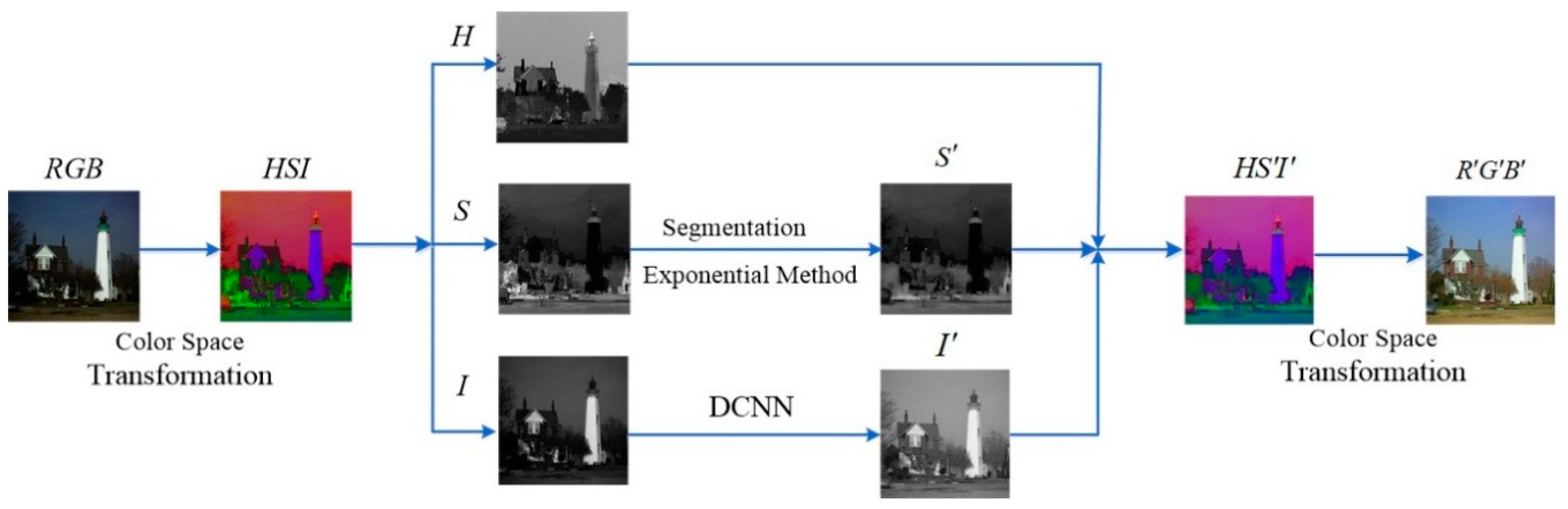
3.1. The Overall Framework of Our Mehod
3.2. Saturation Component Enhancement
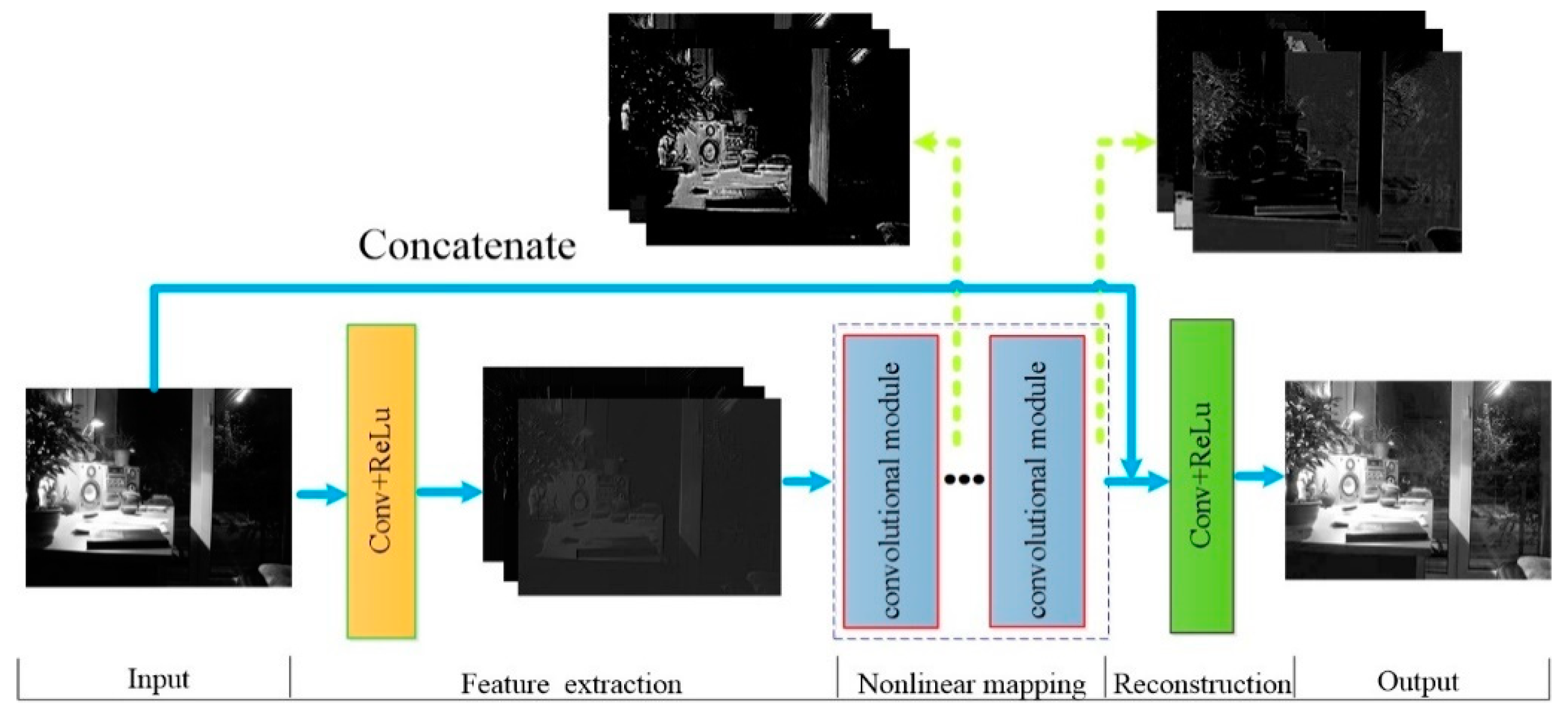
3.3. Intensity Component Enhancement
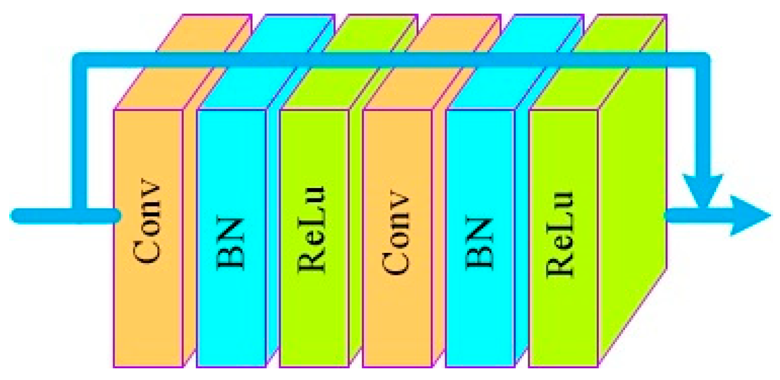
Network Architecture
4. Experiments Results
4.1. Dataset Generation
4.2. Parameter Settings
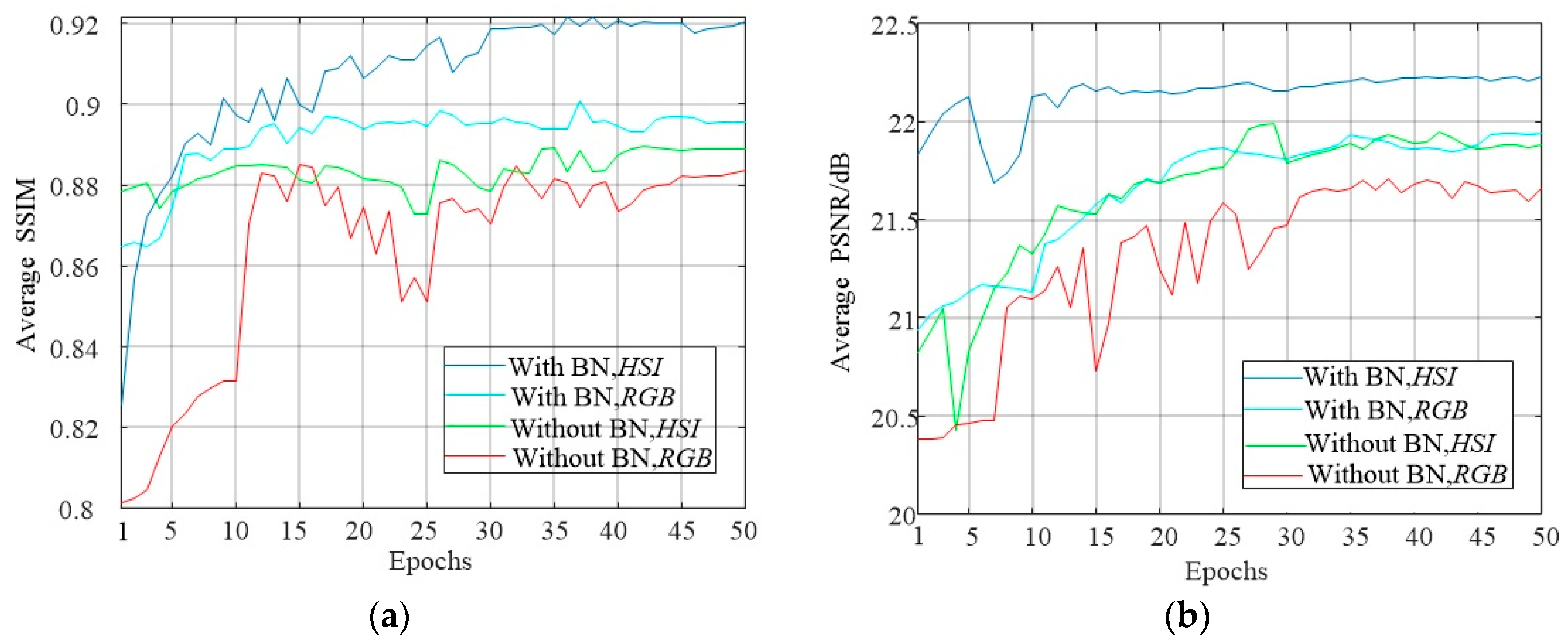
4.3. Study of DCNN Parameters
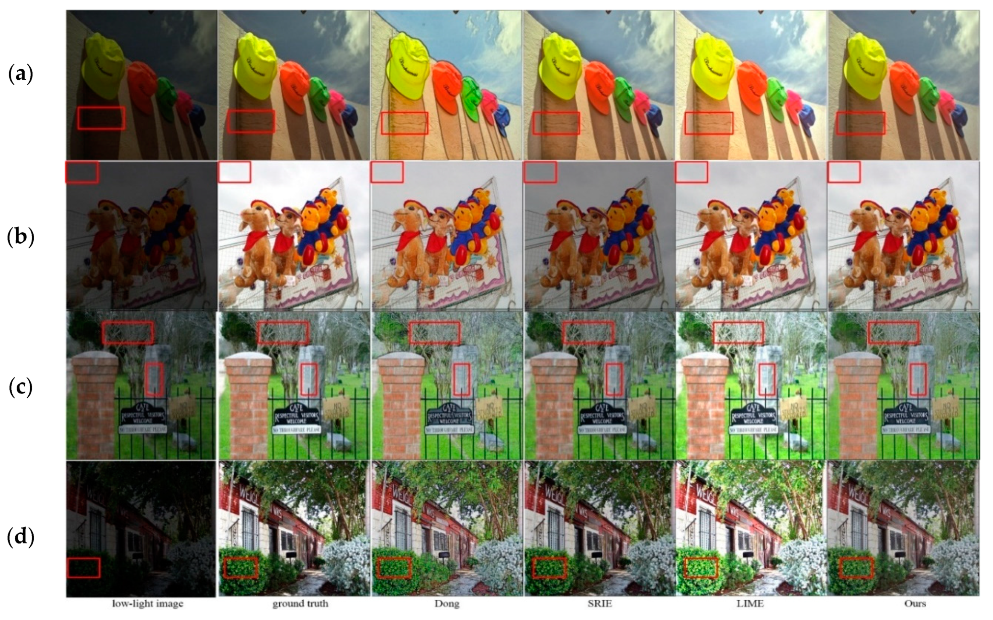
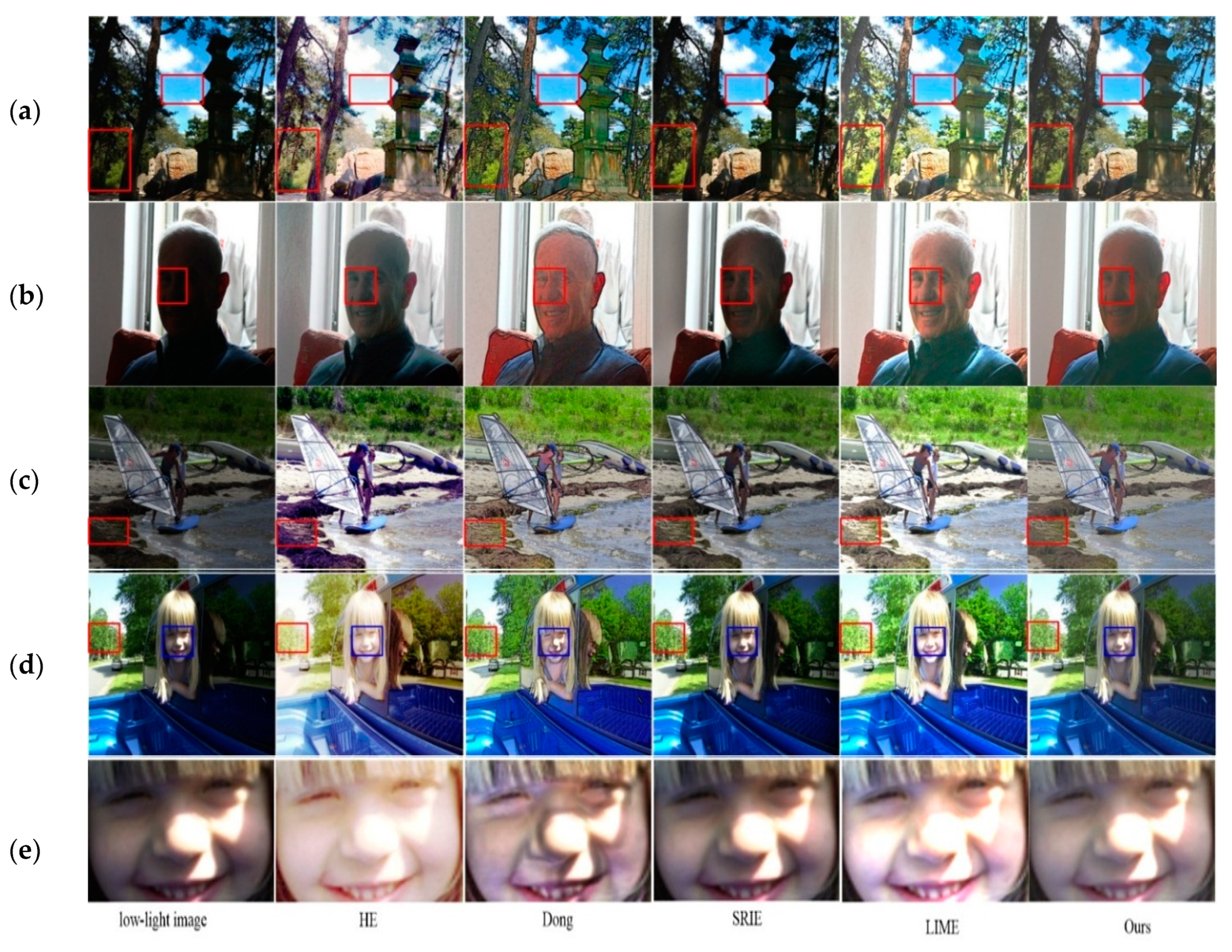
4.4. Comparison with State-of-the-Art Methods
4.4.1. Evaluation on Synthetic Test Dataset
4.4.2. Evaluation on Real-Word Dataset
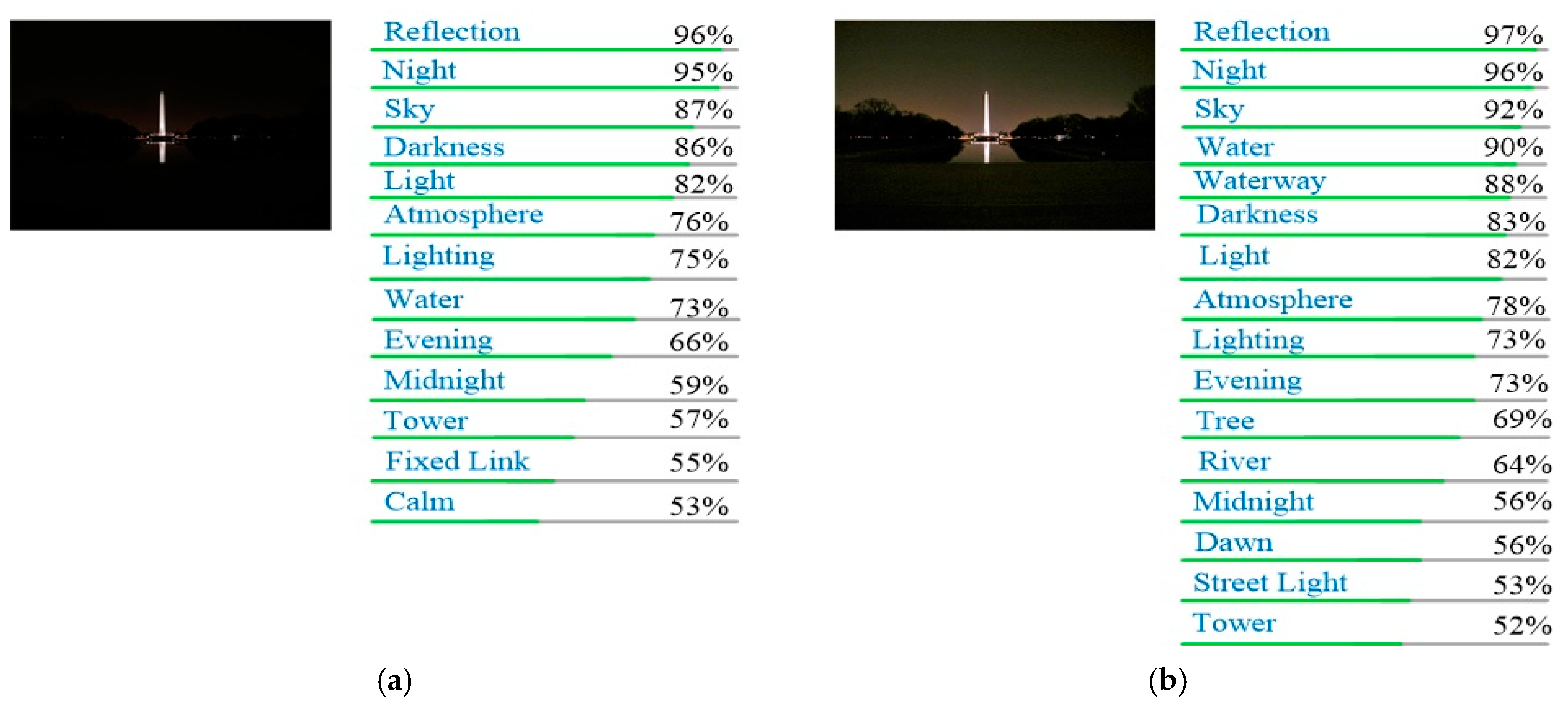
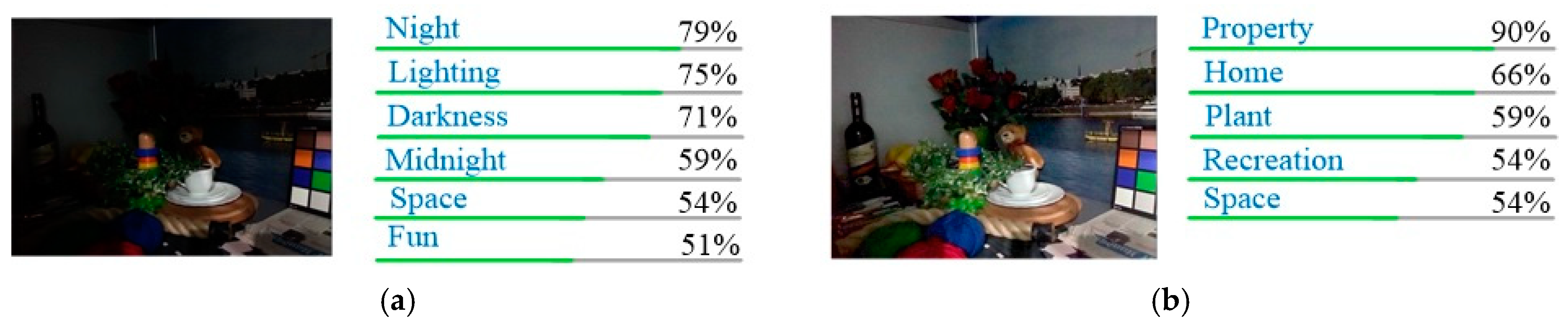
4.5. Application
5. Conclusions
Author Contributions
Funding
Conflicts of Interest
References
- Helmers, H.; Schellenberg, M. CMOS vs. CCD sensors in speckle interferometry. Opt. Laser Technol. 2003, 35, 587–595. [Google Scholar] [CrossRef]
- Tan, Y.; Li, Q.; Li, Y.; Tian, J. Aircraft detection in high-resolution SAR images based on a gradient textural saliency map. Sensors 2015, 15, 23071–23094. [Google Scholar] [CrossRef] [PubMed]
- Pizer, S.M.; Amburn, E.P.; Austin, J.D.; Cromartie, R.; Geselowitz, A.; Greer, T.; ter Haar Romeny, B.; Zimmerman, J.B.; Zuiderveld, K. Adaptive histogram equalization and its variations. Comput. Vis. Graph. Image Process. 1987, 39, 355–368. [Google Scholar] [CrossRef]
- Pisano, E.D.; Zong, S.; Hemminger, B.M. Contrast Limited Adaptive Histogram Equalization image processing to improve the detection of simulated spiculations in dense mammograms. J. Digit. Imaging 1998, 11, 193–200. [Google Scholar] [CrossRef] [PubMed]
- Edwin, H.L. The retinex theory of color vision. Sci. Am. 1977, 237, 108–129. [Google Scholar]
- Zhang, S.; Wang, T.; Dong, J.Y.; Yu, H. Underwater Image Enhancement via Extended Multi-Scale Retinex. Neurocomputing 2017, 245, 1–9. [Google Scholar] [CrossRef]
- Jobson, D.J.; Rahman, Z.; Woodell, G.A. A multiscale retinex for bridging the gap between color images and the human observation of scenes. IEEE Trans. Image Process. 1997, 6, 965–976. [Google Scholar] [CrossRef] [PubMed]
- Fu, X.Y.; Zeng, D.; Huang, Y.; Zhang, X.P.; Ding, X.H. A weighted variational model for simultaneous reflectance and illumination estimation. In Proceedings of the 2016 IEEE Conference on Computer Vision and Pattern Recognition (CVPR), Las Vegas, NV, USA, 26–30 June 2016. [Google Scholar]
- Guo, X.J.; Li, Y.; Ling, H.B. LIME: Low-Light Image Enhancement via Illumination Map Estimation. IEEE Trans. Image Process. 2017, 26, 982–993. [Google Scholar] [CrossRef] [PubMed]
- Hao, S.; Feng, Z.; Guo, Y. Low-light image enhancement with a refined illumination map. Multimed. Tools Appl. 2018, 77, 29639–29650. [Google Scholar] [CrossRef]
- Dong, X.; Wang, G.; Pang, Y.; Li, W.X.; Wen, J.T.; Meng, W.; Liu, Y. Fast efficient algorithm for enhancement of low lighting video. In Proceedings of the International Conference on Multimedia & Expo (ICME 2011), Barcelona, Spain, 11–15 July 2011. [Google Scholar]
- Wu, F.; Kin, T.U. Low-Light image enhancement algorithm based on HSI color space. In Proceedings of the 10th International Congress on Image and Signal Processing, Biomedical Engineering and Informatics (CISP-BMEI 2017), Shanghai, China, 14–16 October 2017. [Google Scholar]
- Nandal, A.; Bhaskar, V.; Dhaka, A. Contrast-based image enhancement algorithm using grey-scale and colour space. IET Signal Process. 2018, 12, 514–521. [Google Scholar] [CrossRef]
- Krizhevsky, A.; Sutskever, I.; Hinton, G.E. ImageNet classification with deep convolutional neural networks. In Proceedings of the 25th International Conference on Neural Information Processing Systems (NIPS), Lake Tahoe, NV, USA, 3–8 December 2012. [Google Scholar]
- Ren, S.Q.; He, K.M.; Girshick, R.; Sun, J. Faster r-cnn: Towards real-time object detection with region proposal networks. In Proceedings of the 28th International Conference on Neural Information Processing Systems (NIPS), Montreal, QC, Canada, 7–12 December 2015; MIT Press: Cambridge, MA, USA, 2015; pp. 91–99. [Google Scholar]
- Wang, L.J.; Ouyang, W.L.; Wang, X.G.; Lu, H.C. Visual tracking with fully convolutional networks. In Proceedings of the IEEE International Conference on Computer Vision (ICCV), CentroParque Convention Center, Santiago, Chile, 7–13 December 2015; IEEE Computer Society: Washington, DC, USA, 2015; pp. 3119–3127. [Google Scholar]
- Lore, K.G.; Akintayo, A.; Sarkar, S. LLNet: A deep autoencoder approach to natural low-light image enhancement. Pattern Recognit. 2017, 61, 650–662. [Google Scholar] [CrossRef]
- Zhang, W.F.; Liang, J.; Ren, L.Y. Fast polarimetric dehazing method for visibility enhancement in HSI colour space. J. Opt. 2017, 19, 095606. [Google Scholar] [CrossRef]
- He, S.F.; Lau, R.W.; Liu, W.X. SuperCNN: A Superpixelwise Convolutional Neural Network for Salient Object Detection. Int. J. Comput. Vis. 2015, 115, 330–344. [Google Scholar] [CrossRef]
- Fu, X.; Huang, J.; Zeng, D. Removing Rain from Single Images via a Deep Detail Network. In Proceedings of the 2017 IEEE Conference on Computer Vision and Pattern Recognition (CVPR), Honolulu, HI, USA, 21–26 July 2017; pp. 1715–1723. [Google Scholar]
- Glorot, X.; Bordes, A.; Bengio, Y. Deep sparse rectifier neural networks. In Proceedings of the 14th International Conference on Artificial Intelligence and Statistics (AISTATS), Fort Lauderdale, FL, USA, 11–13 April 2011. [Google Scholar]
- Huang, G.; Liu, Z. Densely Connected Convolutional Networks. In Proceedings of the 2017 IEEE Conference on Computer Vision and Pattern Recognition (CVPR), Honolulu, HI, USA, 21–26 July 2017; pp. 2261–2269. [Google Scholar]
- Ioffe, S.; Szegedy, C. Batch Normalization: Accelerating Deep Network Training by Reducing Internal Covariate Shift. PMLR 2015, 37, 448–456. [Google Scholar]
- Li, J.; Feng, J. Deep convolutional neural network for latent fingerprint enhancement. Signal Process. Image Commun. 2017, 60, 52–63. [Google Scholar] [CrossRef]
- Xie, S.; Tu, Z. Holistically-Nested Edge Detection. Int. J. Comput. Vis. 2015, 125, 3–18. [Google Scholar] [CrossRef]
- Vedaldi, A.; Lenc, K. Matconvnet: Convolutional neural networks for matlab. In Proceedings of the 23rd Annual ACM Conference on Multimedia Conference, Brisbane, Australia, 26–30 October 2015. [Google Scholar]
- He, K.; Zhang, X.; Ren, S. Delving Deep into Rectifiers: Surpassing Human-Level Performance on ImageNet Classification. In Proceedings of the 2015 IEEE International Conference on Computer Vision (ICCV) ICCV ’15, Santiago, Chile, 7–13 December 2015; pp. 1026–1034. [Google Scholar]
- Dong, C.; Chen, C.L.; He, K.M. Image Super-Resolution Using Deep Convolutional Networks. IEEE Trans. Pattern Anal. Mach. Intell. 2016, 38, 295–307. [Google Scholar] [CrossRef] [PubMed]
- Gonzalez, R.C.; Woods, R.E. Digital Image Processing; Prentice–Hall: Englewood Cliffs, NJ, USA, 2017. [Google Scholar]
- Sheikh, H.R.; Sabir, M.F.; Bovik, A.C. A Statistical Evaluation of Recent Full Reference Image Quality Assessment Algorithms. IEEE Trans. Image Process. 2006, 15, 3440–3451. [Google Scholar] [CrossRef] [PubMed]
- Wang, S.H.; Zheng, J.; Hu, H.M. Naturalness Preserved Enhancement Algorithm for Non-Uniform Illumination Images. IEEE Trans. Image Process. 2013, 22, 3538–3548. [Google Scholar] [CrossRef] [PubMed]
- NASA. Retinex Image Processing. Available online: http://dragon.larc.nasa.gov/retinex/pao/news/ (accessed on 20 October 2018).
- Lee, C.; Kim, C.S. Contrast enhancement based on layered difference representation. In Proceedings of the 19th IEEE International Conference on Image Processing, Orlando, FL, USA, 30 September–3 October 2012. [Google Scholar]
- Vassilios Vonikakis. Available online: https://sites.google.com/site/vonikakis/datasets (accessed on 20 October 2018).
- Wang, S.; Luo, G. Naturalness Preserved Image Enhancement Using a priori Multi-Layer Lightness Statistics. IEEE Trans. Image Process. 2018, 27, 938–948. [Google Scholar] [CrossRef] [PubMed]
- Liu, J.Y.; Yang, W.H. Joint Denoising and Enhancement for Low-Light Images via Retinex Model. In Proceedings of the 14th International Forum on Digital TV and Wireless Multimedia Communication, Shanghai, China, 8–9 November 2017. [Google Scholar]
- Chow, L.S.; Rajagopal, H.; Paramesran, R. Correlation between subjective and objective assessment of magnetic resonance (MR) images. Magn. Reson. Imaging 2016, 34, 820–831. [Google Scholar] [CrossRef] [PubMed]
- Ying, Z.Q.; Li, G.; Gao, W. A Bio-Inspired Multi-Exposure Fusion Framework for Low-Light Image Enhancement. Available online: https://github.com/baidut/BIMEF (accessed on 20 October 2018).


| Layers | Filters Numbers | PSNR | LOE |
|---|---|---|---|
| 5 | 21.74 | 401 | |
| 5 | 21.87 | 394 | |
| 7 | 22.23 | 371 | |
| 7 | 22.31 | 365 | |
| 9 | 22.04 | 383 | |
| 9 | 22.17 | 378 |
| Method | HE | Dong | SRIE | LIME | Ours |
|---|---|---|---|---|---|
| PSNR | 16.19 | 16.29 | 21.08 | 13.47 | 21.33 |
| SSIM | 0.7985 | 0.7947 | 0.9579 | 0.8097 | 0.9204 |
| MSE | 1928.3 | 1699.6 | 686.4 | 3230.7 | 389 |
| LOE | 505 | 2040 | 776 | 1277 | 402 |
| Method | HE | Dong | SRIE | LIME | Ours |
| entropy | 7.1412 | 6.9541 | 6.9542 | 7.2612 | 7.1425 |
| Chromaticity change | 0.2474 | 0.0313 | 0.0045 | 0.0124 | 0.0032 |
| LOE | 571 | 1484 | 972 | 1390 | 378 |
| VIF | 0.4782 | 0.4262 | 0.6153 | 0.3444 | 0.7356 |
© 2018 by the authors. Licensee MDPI, Basel, Switzerland. This article is an open access article distributed under the terms and conditions of the Creative Commons Attribution (CC BY) license (http://creativecommons.org/licenses/by/4.0/).
Share and Cite
Ma, S.; Ma, H.; Xu, Y.; Li, S.; Lv, C.; Zhu, M. A Low-Light Sensor Image Enhancement Algorithm Based on HSI Color Model. Sensors 2018, 18, 3583. https://doi.org/10.3390/s18103583
Ma S, Ma H, Xu Y, Li S, Lv C, Zhu M. A Low-Light Sensor Image Enhancement Algorithm Based on HSI Color Model. Sensors. 2018; 18(10):3583. https://doi.org/10.3390/s18103583
Chicago/Turabian StyleMa, Shiping, Hongqiang Ma, Yuelei Xu, Shuai Li, Chao Lv, and Mingming Zhu. 2018. "A Low-Light Sensor Image Enhancement Algorithm Based on HSI Color Model" Sensors 18, no. 10: 3583. https://doi.org/10.3390/s18103583
APA StyleMa, S., Ma, H., Xu, Y., Li, S., Lv, C., & Zhu, M. (2018). A Low-Light Sensor Image Enhancement Algorithm Based on HSI Color Model. Sensors, 18(10), 3583. https://doi.org/10.3390/s18103583