Validation of an Improved Statistical Theory for Sea Surface Whitecap Coverage Using Satellite Remote Sensing Data


Abstract
1. Introduction
2. Model Description
2.1. Parametric Expressions of Whitecap Coverage
2.2. Theoretical Expressions of the Whitecap Coverage for the General Sea State
3. Validation
3.1. Data
3.2. θ and ρ
3.3. Model Analysis
4. Discussion and Conclusions
4.1. Discussion
4.2. Conclusions
Author Contributions
Acknowledgments
Conflicts of Interest
References
- Romero, L.; Lenain, L.; Melville, W.K. Observations of Surface-Wave-Current Interaction. J. Phys. Oceanogr. 2017, 47, 615–632. [Google Scholar] [CrossRef]
- Phillips, O.M.; Weyl, P.K. The Dynamics of the Upper Ocean, 2nd ed.; Cambridge University Press: New York, NY, USA, 1977; p. 344. ISBN 9780521214216. [Google Scholar]
- Zhang, S.; Cao, R.; Xie, L. Energy dissipation through wind-generated breaking waves. Chin. J. Oceanol. Limnol. 2012, 30, 822–825. [Google Scholar] [CrossRef]
- He, H.L.; Song, J.B. Determining the onset and strength of unforced wave breaking in a numerical wave tank. China Ocean Eng. 2014, 28, 501–509. [Google Scholar] [CrossRef]
- Cardone, V.J. Specification of the Wind Distribution in the Marine Boundary Layer for Wave Forecasting. Ph.D. Thesis, New York University, New York, NY, USA, 1970. [Google Scholar]
- Monahan, E.C.; O’Muircheartaigh, I.G. Whitecaps and the passive remote sensing of the ocean surface. Int. J. Remote Sens. 1986, 7, 627–642. [Google Scholar] [CrossRef]
- Kraan, G.; Oost, W.A.; Janssen, P.A.E.M. Wave Energy Dissipation by Whitecaps. J. Atmos. Ocean. Technol. 1996, 13, 262. [Google Scholar] [CrossRef]
- Cavaleri, L.; Alves, J.H.; Ardhuin, F.; Babanin, A.; Banner, M.; Belibassakis, K.; Benoit, M.; Donelan, M.; Groeneweg, J.; Herbers, T.H.; et al. Wave modelling—The state of the art. Prog. Oceanogr. 2007, 75, 603–674. [Google Scholar] [CrossRef]
- Thomson, J.; Gemmrich, J.R.; Jessup, A.T. Energy dissipation and the spectral distribution of whitecaps. Geophys. Res. Lett. 2009, 36, 192–200. [Google Scholar] [CrossRef]
- Lamarre, E.; Melville, W.K. Air entrainment and dissipation in breaking waves. Nature 1991, 351, 469–472. [Google Scholar] [CrossRef]
- Melville, W.K.; Loewen, M.R.; Lamarre, E. Sound Production and Air Entrainment by Breaking Waves: A Review of Recent Laboratory Experiments. In Breaking Waves; Banner, M.L., Grimshaw, R.H.J., Eds.; Springer: Berlin/Heidelberg, Germany, 1992; pp. 139–146. ISBN 9783642848490. [Google Scholar]
- Zhao, D.L. Progress in sea spay and its effects on air-sea interaction. Adv. Earth Sci. 2012, 27, 624–632. [Google Scholar]
- Monahan, E.C. Whitecap Coverage as a Remotely Monitorable Indication of the Rate of Bobbie Injection into the Oceanic Mixed Layer. In Sea Surface Sound; Bryan, R.K., Ed.; Springer: Berlin/Heidelberg, Germany, 1988; Volume 238, pp. 85–96. ISBN 9789401078566. [Google Scholar]
- Monahan, E.C. Occurrence and evolution of acoustically relevant subsurface bubble plumes and their associated, remotely monitoriable, surface whitecaps. In Natural Physical Sources of Underwater Sound; Kerman, B., Ed.; Kluwer Academic Publishers: Dordrecht, The Netherlands, 1990; pp. 503–524. [Google Scholar]
- Potter, H.; Smith, G.B.; Snow, C.M.; Dowgiallo, D.J.; Bobak, J.P.; Anguelova, M.D. Whitecap lifetime stages from infrared imagery with implications for microwave radiometric measurements of whitecap fraction. J. Geophys. Res. 2016, 120, 7521–7537. [Google Scholar] [CrossRef]
- Randolph, K.; Dierssen, H.M.; Cifuentes-Lorenzen, A.; Balch, W.M.; Monahan, E.C.; Zappa, C.J.; Drapeau, D.T.; Bowler, B. Novel methods for optically measuring whitecaps under natural wave breaking conditions in the Southern Ocean. J. Atmos. Ocean. Technol. 2016, 34, 533–554. [Google Scholar] [CrossRef]
- Callaghan, A.; de Leeuw, G.; Cohen, L.; O’Dowd, C.D. Relationship of oceanic whitecap coverage to wind speed and wind history. Geophys. Res. Lett. 2008, 35, 285–295. [Google Scholar] [CrossRef]
- Dyachenko, S.; Newell, A.C. Whitecapping. Stud. Appl. Math. 2016, 137, 199–213. [Google Scholar] [CrossRef]
- Anguelova, M.D.; Webster, F. Whitecap coverage from satellite measurements: A first step toward modeling the variability of oceanic whitecaps. J. Geophys. Res. 2006, 111, C03–C017. [Google Scholar] [CrossRef]
- Salisbury, D.J.; Anguelova, M.D.; Brooks, I.M. On the variability of whitecap fraction using satellite-based observations. J. Geophys. Res. 2013, 118, 6201–6222. [Google Scholar] [CrossRef]
- Gordon, H.R. Atmospheric correction of ocean color imagery in the Earth Observing System era. J. Geophys. Res. 1997, 102, 17081–17106. [Google Scholar] [CrossRef]
- Frouin, R.; Iacobellis, S.F.; Deschamps, P.Y. Influence of oceanic whitecaps on the Global Radiation Budget. Geophys. Res. Lett. 2001, 28, 1523–1526. [Google Scholar] [CrossRef]
- Monahan, E.C.; Spillane, M.C. The Role of Oceanic Whitecaps in Air-Sea Gas Exchange. In Gas Transfer at Water Surfaces; Brutsaert, W., Jirka, G.H., Eds.; Springer: Berlin/Heidelberg, Germany, 1984; Volume 2, pp. 495–503. ISBN 9789048183937. [Google Scholar]
- Woolf, D.K. Bubbles and their role in gas exchange. In The Sea Surface and Global Change; Liss, P.S., Duce, R.A., Eds.; Cambridge University Press: Cambridge, UK, 1997; Volume 2, pp. 173–205. ISBN 9780521562737. [Google Scholar]
- Asher, W.E.; Wanninkhof, R. The effect of bubble-mediated gas transfer on purposeful dual-gaseous tracer experiments. J. Geophys. Res. 1998, 103, 10555–10560. [Google Scholar] [CrossRef]
- Woolf, D.K.; Leifer, I.S.; Nightingale, P.D.; Rhee, T.S.; Bowyer, P.; Caulliez, G.; De Leeuw, G.; Larsen, S.E.; Liddicoat, M.; Baker, J.; et al. Modelling of bubble-mediated gas transfer: Fundamental principles and a laboratory test. J. Mar. Syst. 2007, 66, 71–91. [Google Scholar] [CrossRef]
- Woolf, D.K. Parametrization of gas transfer velocities and sea-state-dependent wave breaking. Tellus 2005, 57, 87–94. [Google Scholar] [CrossRef]
- Guan, C.L.; Sun, J. Similarities of some wind input and dissipation source terms. China Ocean Eng. 2004, 18, 629–642. [Google Scholar]
- Guan, C.L.; Hu, W.; Sun, J.; Li, R. The whitecap coverage model from breaking dissipation parametrizations of wind waves. J. Geophys. Res. 2007, 112, 395–412. [Google Scholar] [CrossRef]
- Yuan, Y.; Han, L.; Hua, F.; Zhang, S.; Qiao, F.; Yang, Y.; Xia, C. The statistical theory of breaking entrainment depth and surface whitecap coverage of real sea waves. J. Phys. Oceanogr. 2009, 39, 143–161. [Google Scholar] [CrossRef]
- Anguelova, M.D.; Hwang, P.A. Using Energy Dissipation Rate to Obtain Active Whitecap Fraction. J. Phys. Oceanogr. 2015, 46, 461–481. [Google Scholar] [CrossRef]
- Wang, H.; Yang, Y.; Sun, B.; Shi, Y. Improvements to the statistical theoretical model for wave breaking based on the ratio of breaking wave kinetic and potential energy. Sci. China Earth Sci. 2017, 59, 1–8. [Google Scholar] [CrossRef]
- Monahan, E.C. Oceanic whitecaps. J. Phys. Oceanogr. 1971, 1, 139–144. [Google Scholar] [CrossRef]
- Monahan, E.C.; Muircheartaigh, I. Optimal Power-Law Description of Oceanic Whitecap Coverage Dependence on Wind Speed. J. Phys. Oceanogr. 1980, 10, 2094–2099. [Google Scholar] [CrossRef]
- Spillane, M.C.; Monahan, E.C.; Bowyer, P.A.; Doyle, D.M.; Stabeno, P.J. Whitecaps and Global Fluxes. In Oceanic Whitecaps; Monahan, E.C., Niocaill, G.M., Eds.; Springer: Dordrecht, The Netherlands, 1986; Volume 2, pp. 209–218. ISBN 9789401085755. [Google Scholar]
- Bortkovskiĭ, R.S.; Monahan, E.C. AirSea Exchange of Heat and Moisture during Storms. Atmos. Sci. Libr. 1987, 24, 89–112. [Google Scholar]
- Wu, J. Variations of Whitecap Coverage with Wind Stress and Water Temperature. J. Phys. Oceanogr. 1988, 18, 1448–1453. [Google Scholar] [CrossRef]
- Hanson, J.L.; Phillips, O.M. Wind Sea Growth and Dissipation in the Open Ocean. J. Phys. Oceanogr. 1999, 29, 1633–1648. [Google Scholar] [CrossRef]
- Reising, S.C.; Asher, W.E.; Rose, L.A.; Aziz, M.A. Passive Polarimetric Remote Sensing of the Ocean Surface: The Effects of Surface Roughness and Whitecaps. Presented at the International Union of Radio Science, Maastricht, The Netherlands, 17–24 August 2002. [Google Scholar]
- Stramska, M.; Petelski, T. Observations of oceanic whitecaps in the north polar waters of the Atlantic. J. Geophys. Res. 2003, 4504, 1121–1142. [Google Scholar] [CrossRef]
- Villarino, R.; Camps, A.; Vall-Ilossera, M.; Miranda, J.; Arenas, J. Sea foam effects on the brightness temperature at L-band. In Proceedings of the Geoscience and Remote Sensing Symposium, IGARSS ′03, Toulouse, France, 21–25 July 2003. [Google Scholar]
- Lafon, C.; Piazzola, J.; Forget, P.; Le Calve, O.; Despiau, S. Analysis of the Variations of the Whitecap Fraction as Measured in a Coastal Zone. Bound-Lay. Meteorol. 2004, 111, 339–360. [Google Scholar] [CrossRef]
- Goddijnmurphy, L.; Woolf, D.K.; Callaghan, A.H. Parameterizations and Algorithms for Oceanic Whitecap Coverage. J. Phys. Oceanogr. 2011, 41, 742–756. [Google Scholar] [CrossRef]
- Sugihara, Y.; Tsumori, H.; Ohga, T.; Yoshioka, H.; Serizawa, S. Variation of whitecap coverage with wave-field conditions. J. Mar. Syst. 2007, 66, 47–60. [Google Scholar] [CrossRef]
- Zhao, D.; Toba, Y. Dependence of Whitecap Coverage on Wind and Wind-Wave Properties. J. Oceanogr. 2001, 57, 603–616. [Google Scholar] [CrossRef]
- Kinsman, B. Wind waves: Their generation and propagation on the ocean surface. Fungal Biol.-UK 1965, 119, 859–869. [Google Scholar]
- Jones, I.S.F.; Toba, Y. Wind Stress over the Ocean; Cambridge University Press: Cambridge, UK, 2001; p. 307. ISBN 0521662435. [Google Scholar]
- Yang, Y.Z.; Qiao, F.L.; Pan, Z.D. Wave Assimilation and Numerical Prediction. Chin. J. Oceanol. Limnol. 2000, 18, 301–308. [Google Scholar]
- Yang, Y.; Ji, Y.; Yuan, Y. The nonlinear interaction process in the wave assimilation model and its experiments. Chin. J. Oceanol. Limnol. 2003, 21, 18–26. [Google Scholar]
- Jiang, X.; Wang, D.; Gao, D.; Zhang, T. Experiments on exactly computing non-linear energy transfer rate in MASNUM-WAM. Chin. J. Oceanol. Limnol. 2016, 34, 821–834. [Google Scholar] [CrossRef]
- Yang, Y.Z.; Qiao, F.L.; Zhao, W.; Teng, Y.; Yuan, Y. MASNUM ocean wave numerical model in spherical coordinates and its application. Acta Oceanol. Sin. 2005, 27, 1–7. [Google Scholar]
- Anguelova, M.D.; Bobak, J.P.; Asher, W.E.; Dowgiallo, D.J.; Moat, B.I.; Pascal, R.W.; Yelland, M.J. Validation of satellite-based estimates of whitecap coverage: Approaches and initial results. In Proceedings of the 16th Air-Sea Interaction Conference, AMS, Phoenix, AZ, USA, 11–15 January 2009. [Google Scholar]
- Anguelova, M.D.; Gaiser, P.W. Microwave emissivity of sea-foam layers with vertical profile of dielectric properties. Remote Sens. Environ. 2013, 139, 81–96. [Google Scholar] [CrossRef]
- Data. Available online: https://aquarius.oceansciences.org/cgi/data.cgi (accessed on 26 July 2017).
- EMC: Data Assimilation Team. Grid-Point Statistical Interpolation (GSI). Available online: http://www.emc.ncep.noaa.gov/gmb/gdas/ (accessed on 13 May 2016).
- Nordberg, W.; Conaway, J.; Ross, D.B.; Wilheit, T. Measurements of Microwave Emission from a Foam-Covered, Wind-Driven Sea. J. Atmos. Sci. 1971, 28, 429–435. [Google Scholar] [CrossRef]
- Ross, D.B.; Cardone, V. Observations of oceanic whitecaps and their relation to remote measurements of surface wind Speed. J. Geophys. Res. 1974, 79, 444–452. [Google Scholar] [CrossRef]
- Monahan, E.C.; Fairall, C.W.; Davidson, K.L.; Boyle, P.J. Observed interrelation between 10 m winds, ocean whitecaps and marine aerosols. Q. J. R. Meteorol. Soc. 1983, 109, 379–392. [Google Scholar] [CrossRef]
- Scanlon, B.; Breivik, Ø.; Bidlot, J.R.; Janssen, P.A.; Callaghan, A.H.; Ward, B. Modeling Whitecap Fraction with a Wave Model. J. Phys. Oceanogr. 2015, 46, 887–894. [Google Scholar] [CrossRef]


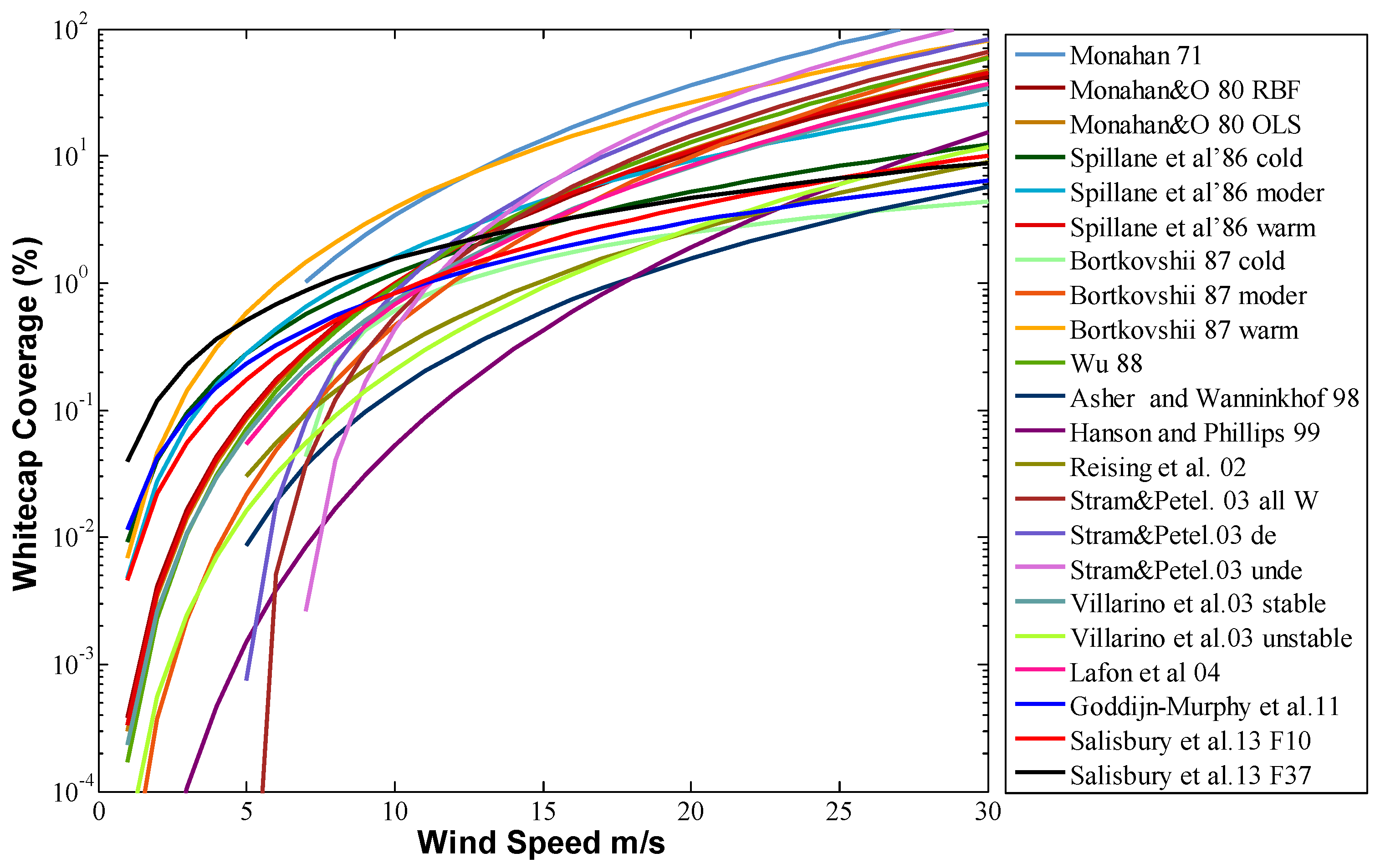
| No. | Reference | As Referred to in Figure 1 | Equation | Note |
|---|---|---|---|---|
| 1 | Monahan [33] | Monahan 71 | As a percentage, U > 7 m/s | |
| 2 | Monahan and O’Muircheartaigh [34] | Monahan & O 80 RBF | ||
| 3 | Monahan and O’Muircheartaigh [34] | Monahan & O 80 OLS | ||
| 4 | Spillane et al. [35] | Spillane et al.’ 86 cold | ||
| 5 | Spillane et al. [35] | Spillane et al.’ 86 moder | ||
| 6 | Spillane et al. [35] | Spillane et al.’ 86 warm | ||
| 7 | Bortkovskii [36] | Bortkovshii 87 cold | As a percentage | |
| 8 | Bortkovskii [36] | Bortkovshii 87 moder | A percentage | |
| 9 | Bortkovskii [36] | Bortkovshii 87 warm | As a percentage | |
| 10 | Wu [37] | Wu 88 | ||
| 11 | Asher and Wanninkhof [25] | Asher and Wanninkhof 98 | ||
| 12 | Hanson and Phillips [38] | Hanson and Phillips 99 | ||
| 13 | Reising et al. [39] | Reising et al. 02 | ||
| 14 | Stramska and Petelski [40] | Stram & Petel. 03 all W | All W measured | |
| 15 | Stramska and Petelski [40] | Stram & Petel. 03 de | Developed sea | |
| 16 | Stramska and Petelski [40] | Stram & Petel. 03 unde | Undeveloped sea | |
| 17 | Villarino et al. [41] | Villarino et al. 03 stable | Stable conditions | |
| 18 | Villarino et al. [41] | Villarino et al. 03 unstable | Unstable conditions | |
| 19 | Lafon et al. [42] | Lafon et al. 04 | As a percentage, U > 5 m/s | |
| 20 | Goddijn et al. [43] | Goddijn-Murphy et al. 11 | ||
| 21 | Salisbury et al. [20] | Salisbury et al. 13 F10 | 10 GHz, horizontal polarization | |
| 22 | Salisbury et al. [20] | Salisbury et al. 13 F37 | 37 GHz, horizontal polarization |
| Model/Sensor Access | Variable | Resolution | Variable Used |
|---|---|---|---|
| Windsat (Coriolis) | Brightness temperature TB (K) | 0.5° × 0.5° | W(TB) algorithm |
| Naval Research Laboratory | |||
| SSM/I (F13) Remote Sensing Systems 1 | Water vapor Cloud liquid water | 0.25° × 0.25° | W(TB) algorithm |
| SeaWinds (QuikSCAT) | Wind speed U10 (m s−1) | 0.25° × 0.25° | W(TB) algorithm |
| PODAAC/JPL 2 | Wind direction Udir (°) | Whitecap coverage expression | |
| MASNUM Wave Model | |||
| GDAS/NCEP 3 | U10, Udir, SST (°C) | 1° × 1° | W(TB) algorithm |
| θ | 8 | 8.6 | 9.2 | 9.8 | 10.4 | 11 | |
|---|---|---|---|---|---|---|---|
| ρ | |||||||
| 0.53 | 1 | 8 | 15 | 22 | 29 | 36 | |
| 0.54 | 2 | 9 | 16 | 23 | 30 | 37 | |
| 0.55 | 3 | 10 | 17 | 24 | 31 | 38 | |
| 0.56 | 4 | 11 | 18 | 25 | 32 | 39 | |
| 0.57 | 5 | 12 | 19 | 26 | 33 | 40 | |
| 0.58 | 6 | 13 | 20 | 27 | 34 | 41 | |
| 0.59 | 7 | 14 | 21 | 28 | 35 | 42 | |
| θ | 8 | 8.6 | 9.2 | 9.8 | 10.4 | 11 | ||
|---|---|---|---|---|---|---|---|---|
| r | ||||||||
| ρ | ||||||||
| 0.53 | 0.6267 | 0.6267 | 0.6265 | 0.6262 | 0.6262 | 0.6262 | ||
| 0.54 | 0.6059 | 0.6059 | 0.6059 | 0.6059 | 0.6059 | 0.6068 | ||
| 0.55 | 0.5835 | 0.5835 | 0.5829 | 0.5821 | 0.5821 | 0.5820 | ||
| 0.56 | 0.5558 | 0.5552 | 0.5546 | 0.5536 | 0.5536 | 0.5530 | ||
| 0.57 | 0.5250 | 0.5250 | 0.5250 | 0.5249 | 0.5249 | 0.5249 | ||
| 0.58 | 0.4977 | 0.4977 | 0.4977 | 0.4979 | 0.4982 | 0.4982 | ||
| 0.59 | 0.4717 | 0.4717 | 0.4717 | 0.4717 | 0.4717 | 0.4710 | ||
| Max (%) | Mean (%) | |
|---|---|---|
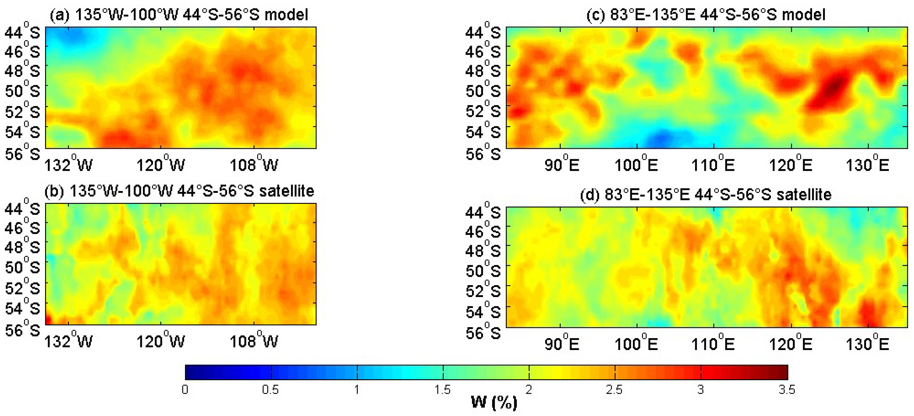
| Model result | 2.966 | 2.227 |
| Satellite result | 3.166 | 2.201 |
| Max (%) | Mean (%) | |
|---|---|---|
| Model result | 3.428 | 2.078 |
| Satellite result | 3.076 | 2.137 |
© 2018 by the authors. Licensee MDPI, Basel, Switzerland. This article is an open access article distributed under the terms and conditions of the Creative Commons Attribution (CC BY) license (http://creativecommons.org/licenses/by/4.0/).
Share and Cite
Wang, H.; Yang, Y.; Dong, C.; Su, T.; Sun, B.; Zou, B. Validation of an Improved Statistical Theory for Sea Surface Whitecap Coverage Using Satellite Remote Sensing Data. Sensors 2018, 18, 3306. https://doi.org/10.3390/s18103306
Wang H, Yang Y, Dong C, Su T, Sun B, Zou B. Validation of an Improved Statistical Theory for Sea Surface Whitecap Coverage Using Satellite Remote Sensing Data. Sensors. 2018; 18(10):3306. https://doi.org/10.3390/s18103306
Chicago/Turabian StyleWang, Haili, Yongzeng Yang, Changming Dong, Tianyun Su, Baonan Sun, and Bin Zou. 2018. "Validation of an Improved Statistical Theory for Sea Surface Whitecap Coverage Using Satellite Remote Sensing Data" Sensors 18, no. 10: 3306. https://doi.org/10.3390/s18103306
APA StyleWang, H., Yang, Y., Dong, C., Su, T., Sun, B., & Zou, B. (2018). Validation of an Improved Statistical Theory for Sea Surface Whitecap Coverage Using Satellite Remote Sensing Data. Sensors, 18(10), 3306. https://doi.org/10.3390/s18103306