A Novel Attitude Determination System Aided by Polarization Sensor

Abstract
:1. Introduction
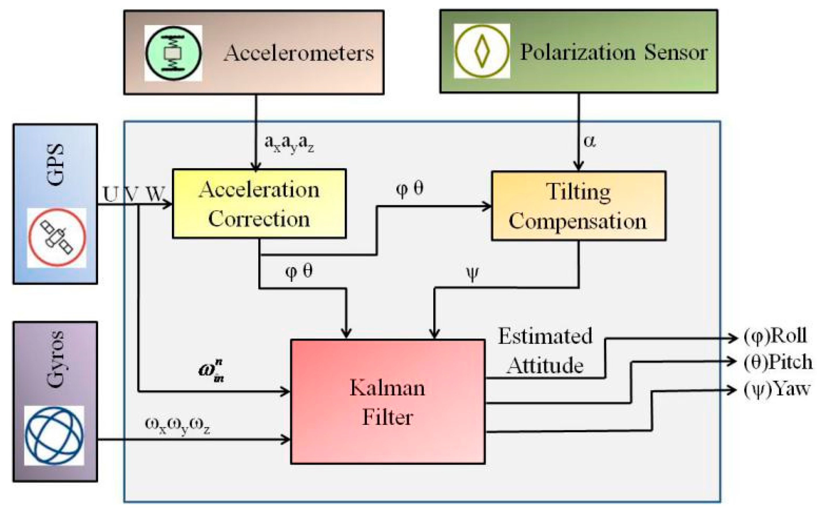
2. System Framework and Coordinates
2.1. System Framework
2.2. Coordinate Systems and Notations
3. Sensor Modeling
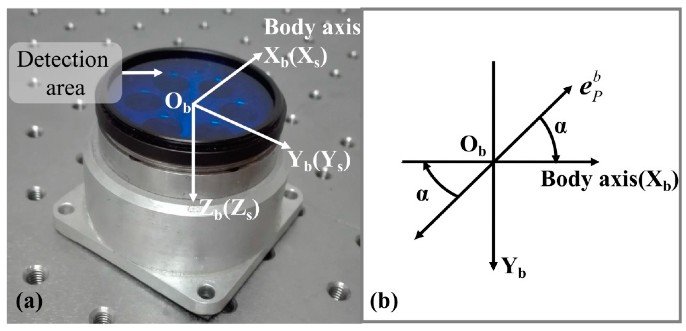
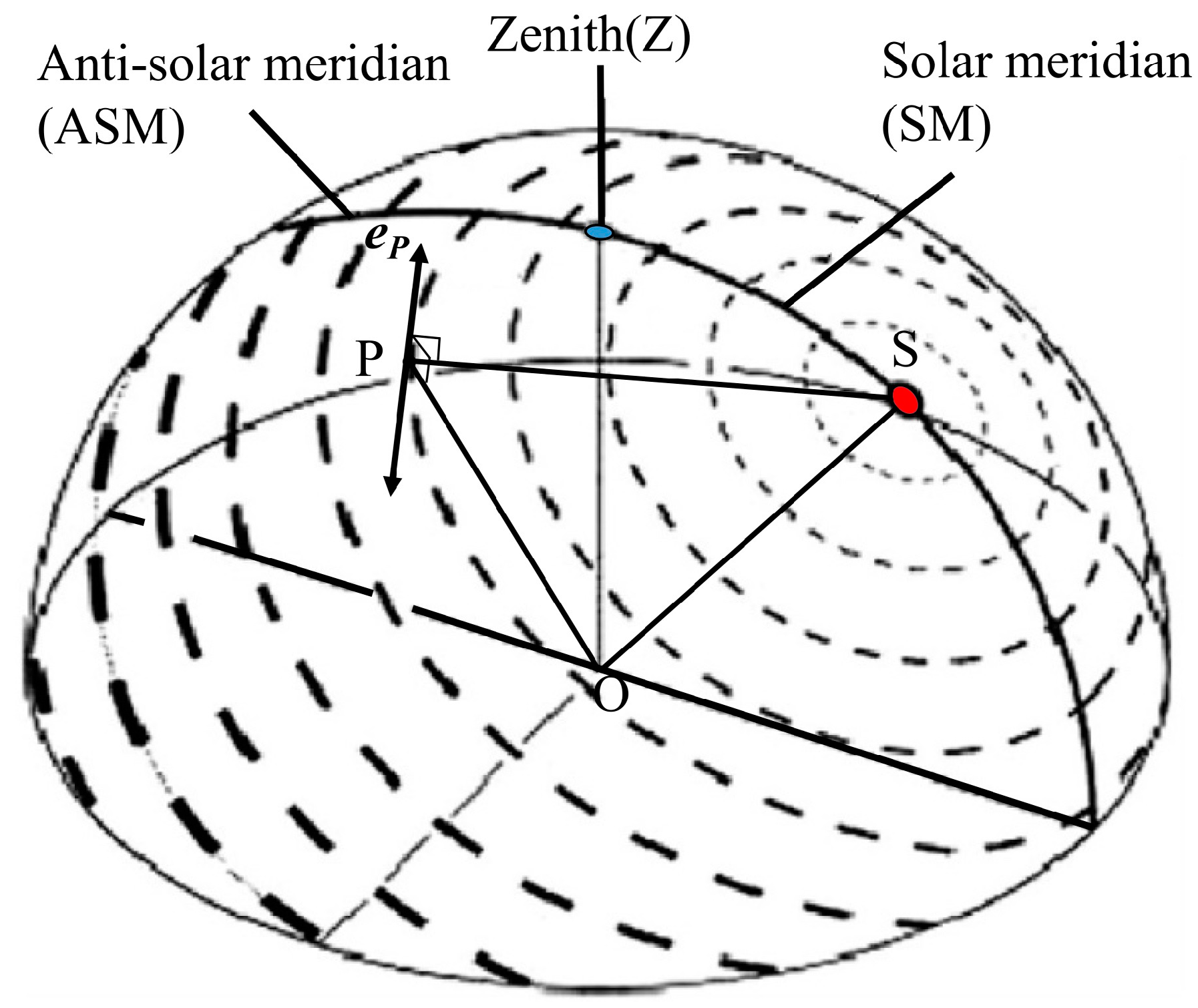
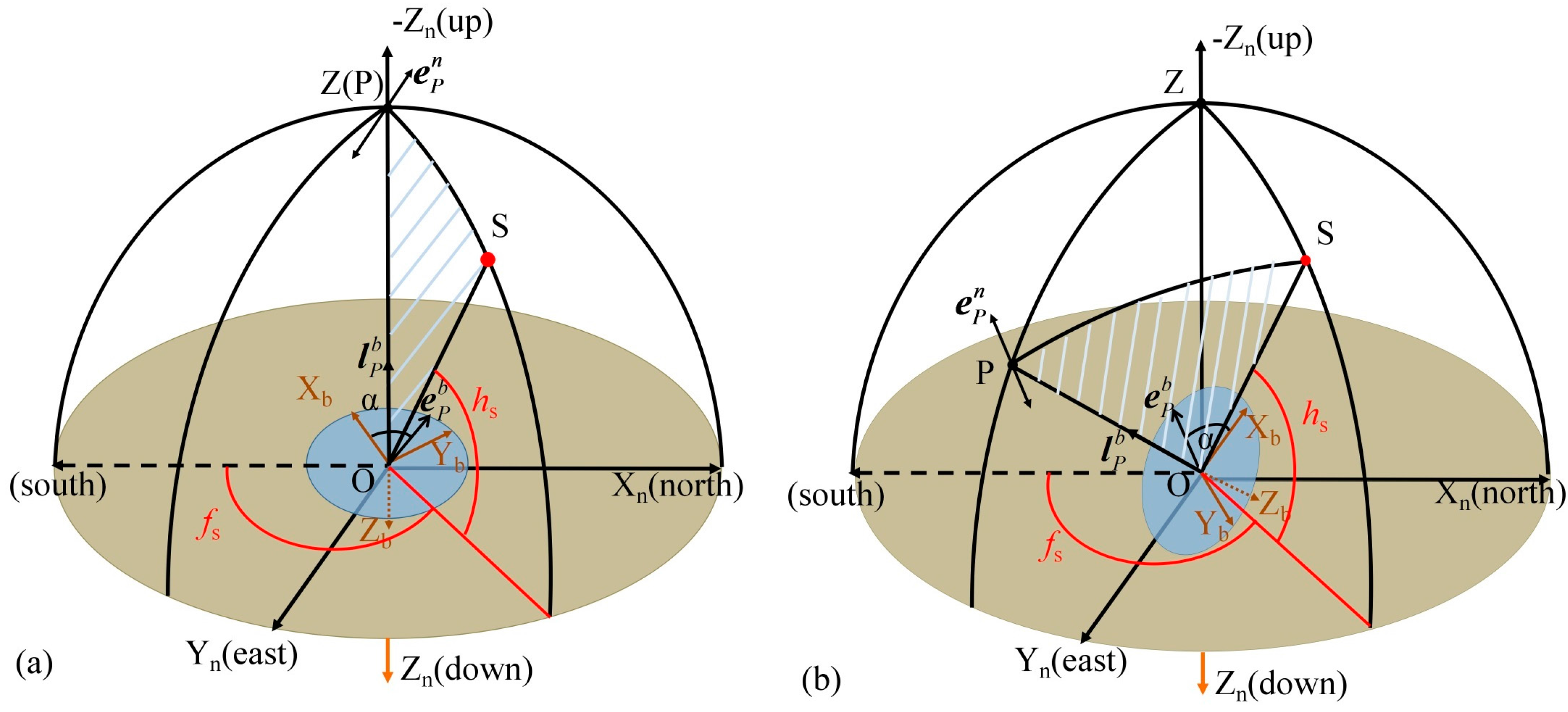
3.1. The Improved Model of Polarization Sensor
3.2. The Attitude Determination Based on Theory of Gravity
4. The Data Fusion Algorithm Based on EKF
4.1. The Kinematical Model Using Quaternion
4.2. State Model and Observation Model of Kalman Filter
4.3. Noise Parameters Determination
5. Experimental Results and Discussion
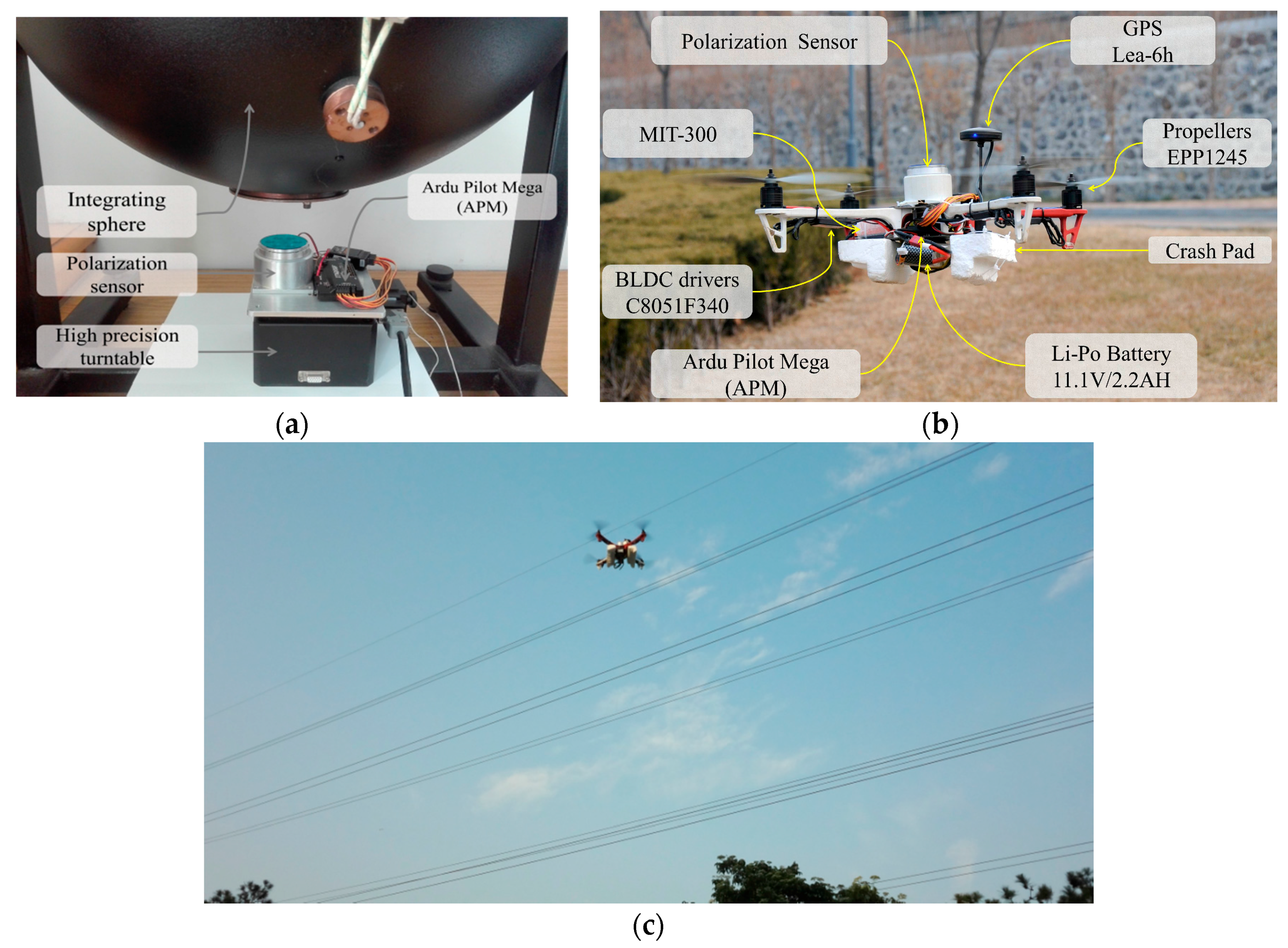
5.1. Hardware Configuration and Scenario Description
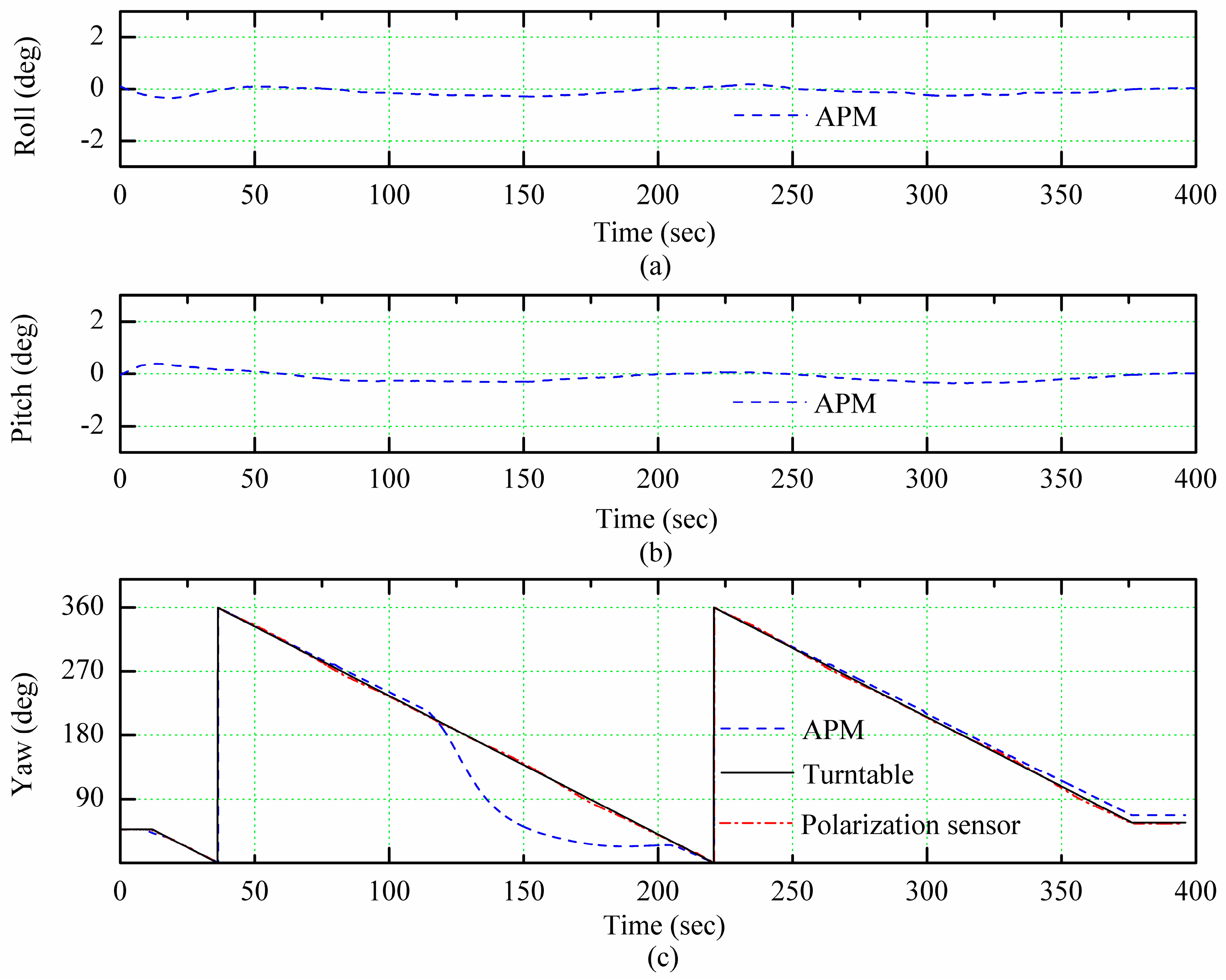
5.2. Indoor Test
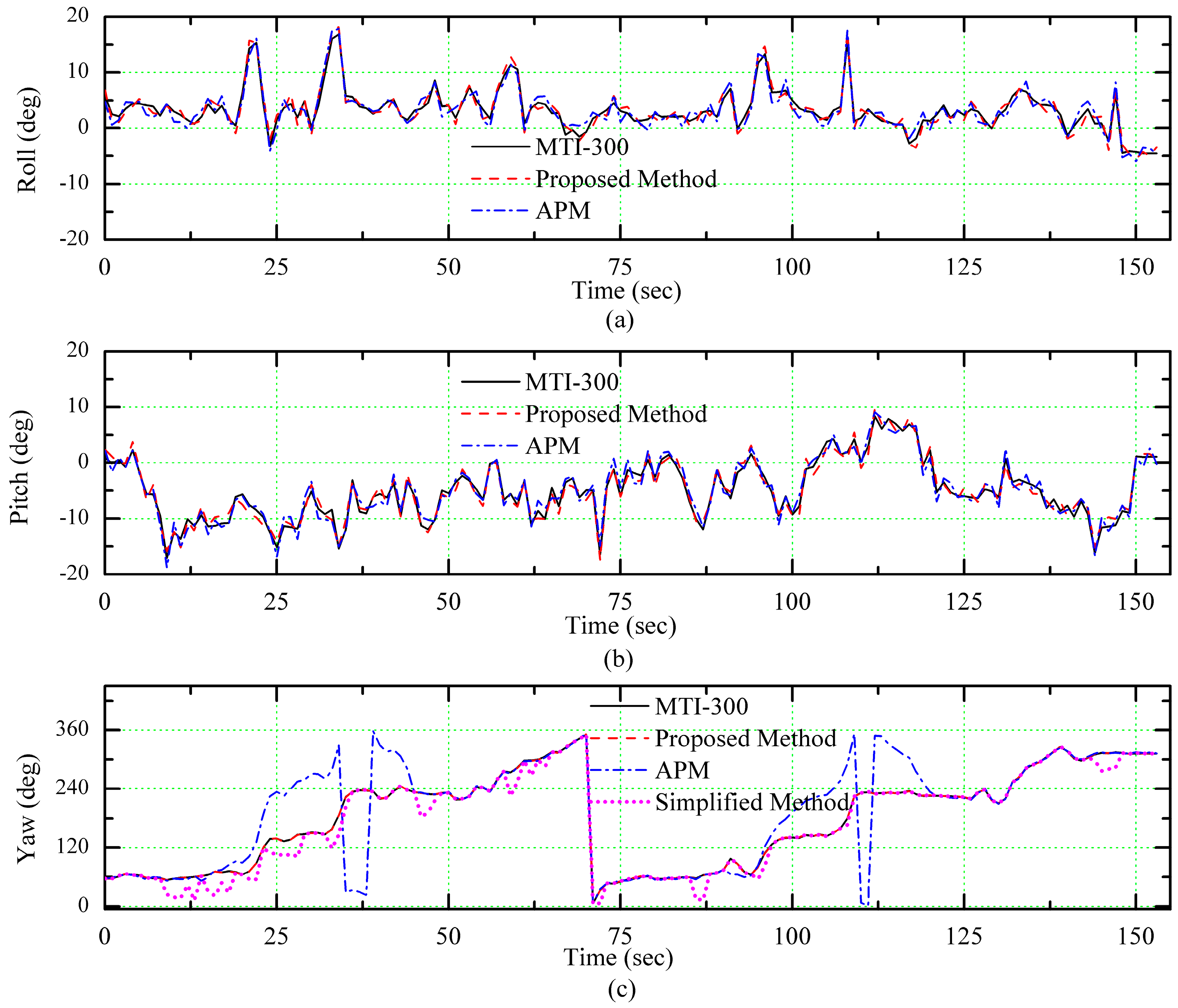
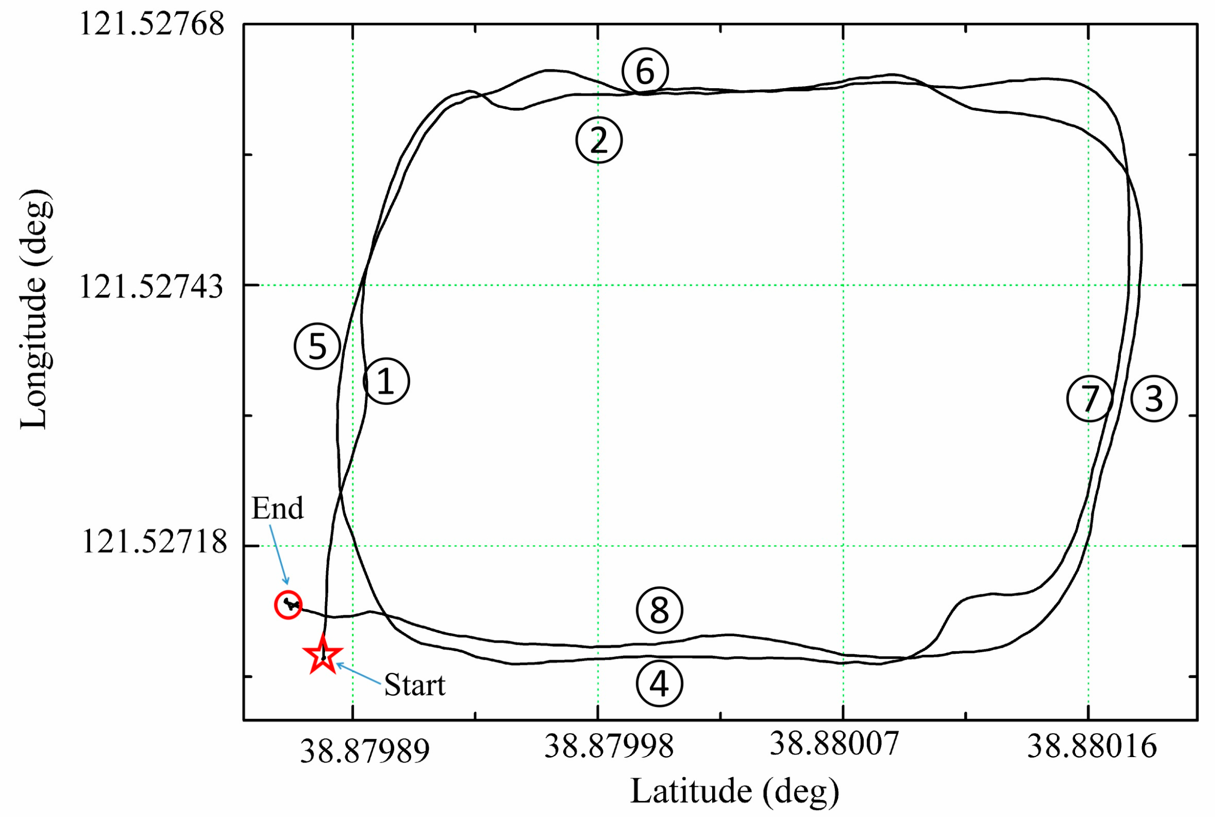
5.3. Outdoor Test
6. Conclusions
Acknowledgments
Author Contributions
Conflicts of Interest
References
- Li, T.; Zhang, H.; Niu, X.; Gao, Z. Tightly-Coupled Integration of Multi-GNSS Single-Frequency RTK and MEMS-IMU for Enhanced Positioning Performance. Sensors 2017, 17, 2462. [Google Scholar] [CrossRef] [PubMed]
- Hinüber, E.L.V.; Reimer, C.; Schneider, T.; Stock, M. INS/GNSS Integration for Aerobatic Flight Applications and Aircraft Motion Surveying. Sensors 2017, 17, 941. [Google Scholar] [CrossRef] [PubMed]
- Eling, C.; Klingbeil, L.; Kuhlmann, H. Real-Time Single-Frequency GPS/MEMS-IMU Attitude Determination of Lightweight UAVs. Sensors 2015, 15, 26212–26235. [Google Scholar] [CrossRef] [PubMed]
- Wang, J.; Yang, G.; Li, J.; Zhou, X. An Anline Gravity Modeling Method Applied for High Precision Free-INS. Sensors 2016, 16, 1541. [Google Scholar] [CrossRef] [PubMed]
- Wang, J.L.; Li, W. Effective Adaptive Kalman Filter for MEMS-IMU/Magnetometers Integrated Attitude and Heading Reference Systems. J. Navig. 2013, 66, 99–113. [Google Scholar]
- Yoo, T.S.; Hong, S.K.; Yoon, H.M.; Park, S. Gain-Scheduled Complementary Filter Design for a MEMS Based Attitude and Heading Reference System. Sensors 2011, 11, 3816–3830. [Google Scholar] [CrossRef] [PubMed]
- Han, S.; Wang, J. A Novel Method to Integrate IMU and Magnetometers in Attitude and Heading Reference Systems. J. Navig. 2011, 64, 727–738. [Google Scholar] [CrossRef]
- Lambrinos, D.; Kobayashi, H.; Pfeifer, R.; Maris, M.; Labhart, T.; Wehner, R. An Autonomous Agent Navigating with a Polarized Light Compass. Adapt. Behav. 1997, 6, 131–161. [Google Scholar] [CrossRef]
- Belenkii, M. Celestial Compass with Sky Polarization. U.S. Patent 20,150,042,793, 12 February 2015. [Google Scholar]
- Dacke, M.; Nilsson, D.E.; Scholtz, C.H.; Byrne, M.; Warrant, E.J. Insect Orientation to Polarized Moonlight. Nature 2003, 424, 33. [Google Scholar] [CrossRef] [PubMed]
- Lambrinos, D.; Möller, R.; Labhart, T.; Pfeifer, R.; Wehner, R. A Mobile Robot Employing Insect Strategies for Navigation. Robot. Auton. Syst. 2000, 30, 39–64. [Google Scholar] [CrossRef]
- Chu, J.; Wang, H.; Chen, W.; Li, R. Application of A Novel Polarization Sensor to Mobile Robot Navigation. In Proceedings of the International Conference on Mechatronics and Automation, Changchun, Jilin, China, 9–12 August 2009; pp. 3763–3768. [Google Scholar]
- Kong, X.; Wu, W.; Zhang, L.; He, X.; Wang, Y. Performance Improvement of Visual-Inertial Navigation System by Using Polarized Light Compass. Ind. Robot Int. J. 2016, 43, 588–595. [Google Scholar] [CrossRef]
- Chahl, J.; Mizutani, A. Biomimetic Attitude and Orientation Sensors. IEEE Sens. J. 2012, 12, 289–297. [Google Scholar] [CrossRef]
- Cui, Y.; Chu, J.K.; Cao, N.N.; Zhao, K.C. Study on Measuring System for Characteristics and Distribution of Skylight Polarization. In Key Engineering Materials; Trans Tech Publications: Stafa-Zurich, Switzerland, 2010; Volume 437, pp. 369–373. [Google Scholar]
- Pomozi, I.; Horváth, G.; Wehner, R. How The Clear-Sky Angle of Polarization Pattern Continues Underneath Clouds: Full-Sky Measurements and Implications for Animal Orientation. J. Exp. Biol. 2001, 204, 2933–2942. [Google Scholar] [PubMed]
- Chu, J.; Zhao, K.; Zhang, Q.; Wang, T. Design of a Novel Polarization Sensor for Navigation. In Proceedings of the International Conference on Mechatronics and Automation, Harbin, China, 5–8 August 2007; pp. 3161–3166. [Google Scholar]
- Ma, T.; Hu, X.; Zhang, L.; Lian, J.; He, X.; Wang, Y. An evaluation of skylight polarization patterns for navigation. Sensors 2015, 15, 5895–5913. [Google Scholar] [CrossRef] [PubMed]
- Miyazaki, D.; Ammar, M.; Kawakami, R.; Ikeuchi, K. Estimating Sunlight Polarization Using a Fish-eye Lens. IPSJ Trans. Comput. Vis. Appl. 2010, 1, 288–300. [Google Scholar] [CrossRef]
- Zhi, W. A Novel Attitude and Heading Reference Systems Based on Bionic Polarization Sensors. J. Inf. Comput. Sci. 2015, 12, 5363–5374. [Google Scholar] [CrossRef]
- Ma, D.M.; Shiau, J.K.; Wang, I.C.; Lin, Y.H. Attitude Determination Using a MEMS-Based Flight Information Measurement Unit. Sensors 2012, 12, 1–23. [Google Scholar] [CrossRef] [PubMed]
- Hemerly, E.M.; Maciel, B.C.O.; Milhan, A.D.P.; Schad, V.R. Attitude and Heading Reference System with Acceleration Compensation. Aircr. Eng. Aerosp. Technol. 2012, 84, 87–93. [Google Scholar] [CrossRef]
- Savage, P.G. Strapdown Inertial Navigation Integration Algorithm Design. I: Attitude algorithms. J. Guid. Control Dyn. 2012, 21, 19–28. [Google Scholar] [CrossRef]
- Liang, X.; Yuan, W.Z.; Chang, H.L.; Wei, Q.; Yuan, G.M.; Jiang, C.Y. Application of Quaternion-Based Extended Kalman Filter for MAV Attitude Estimation Using MEMS Sensors. Nanotechnol. Precis. Eng. 2009, 7, 163–167. [Google Scholar]
- Markley, F.L.; Crassidis, J.L. Fundamentals of Spacecraft Attitude Determination and Control, 3rd ed.; Springer: New York, NY, USA, 2014; pp. 237–262. [Google Scholar]
- Premerlani, W.; Bizard, P. Direction Cosine Matrix IMU: Theory. Available online: http://owenson.me/build-your-own-quadcopter-autopilot/DCMDraft2.pdf (accessed on 5 January 2018).
- Chu, J.; Zhao, K.; Zhang, Q.; Wang, T. Construction and Performance Test of a Novel Polarization Sensor for Navigation. Sens. Actuator A Phys. 2008, 148, 75–82. [Google Scholar] [CrossRef]


| Sensors | Product Model | Specifications | Sampling Rates (Hz) |
|---|---|---|---|
| AHRS | MTI-300 | Roll dynamic value: 0.3° | 100 |
| Pitch Dynamic value: 0.3° | |||
| Yaw Dynamic value: 1.0° | |||
| MIMU | MPU6000 | Gyro Sensitivity: 131 LSB/(°/s) Full scale range: ±250°/s | 20 |
| Accelerometer Sensitivity: 4096 LSB/g Full scale range: ±8 g | |||
| Magnetometer | HMC5883 | Typical Noise Floor: 2 milligauss | 10 |
| Polarization sensor | Self-development | Accuracy (indoor): 0.2° Accuracy (outdoor): <2° | 10 |
| Methods | Roll (RMSE) | Pitch (RMSE) | Yaw (RMSE) |
|---|---|---|---|
| APM | 1.93° | 1.89° | 3.01° |
| Proposed Method | 1.87° | 1.85° | 1.25° |
| Simplified Method | Null | Null | 23.10° |
© 2018 by the authors. Licensee MDPI, Basel, Switzerland. This article is an open access article distributed under the terms and conditions of the Creative Commons Attribution (CC BY) license (http://creativecommons.org/licenses/by/4.0/).
Share and Cite
Zhi, W.; Chu, J.; Li, J.; Wang, Y. A Novel Attitude Determination System Aided by Polarization Sensor. Sensors 2018, 18, 158. https://doi.org/10.3390/s18010158
Zhi W, Chu J, Li J, Wang Y. A Novel Attitude Determination System Aided by Polarization Sensor. Sensors. 2018; 18(1):158. https://doi.org/10.3390/s18010158
Chicago/Turabian StyleZhi, Wei, Jinkui Chu, Jinshan Li, and Yinlong Wang. 2018. "A Novel Attitude Determination System Aided by Polarization Sensor" Sensors 18, no. 1: 158. https://doi.org/10.3390/s18010158
APA StyleZhi, W., Chu, J., Li, J., & Wang, Y. (2018). A Novel Attitude Determination System Aided by Polarization Sensor. Sensors, 18(1), 158. https://doi.org/10.3390/s18010158