Practical Use of Metal Oxide Semiconductor Gas Sensors for Measuring Nitrogen Dioxide and Ozone in Urban Environments

 ,
,
Abstract
1. Introduction
1.1. MOS Sensors
1.2. Previous Work from Other Groups
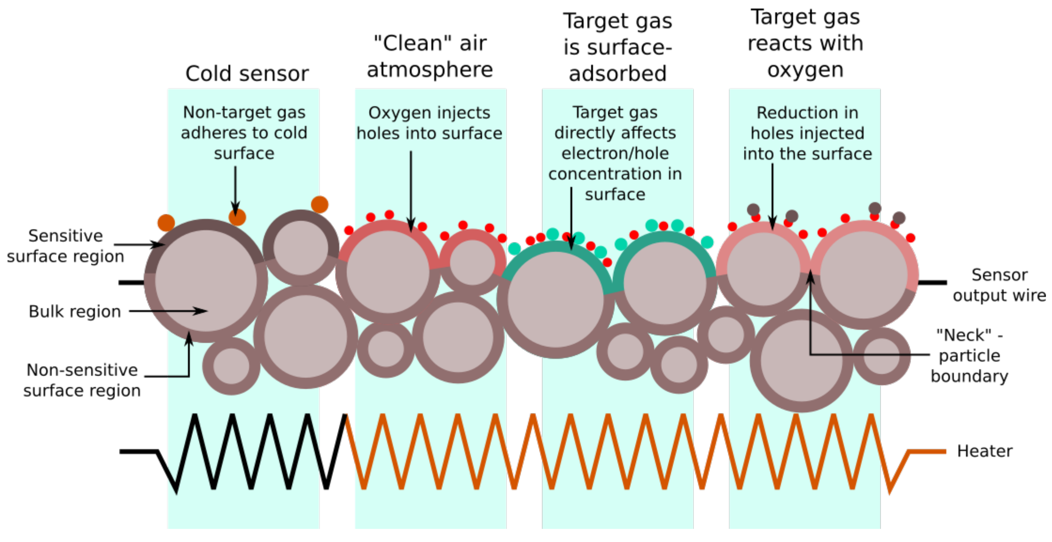
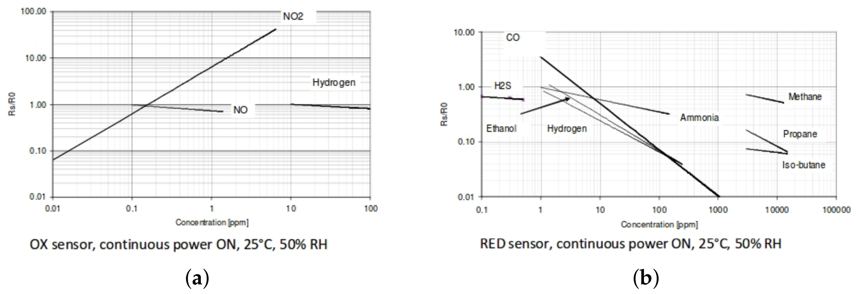
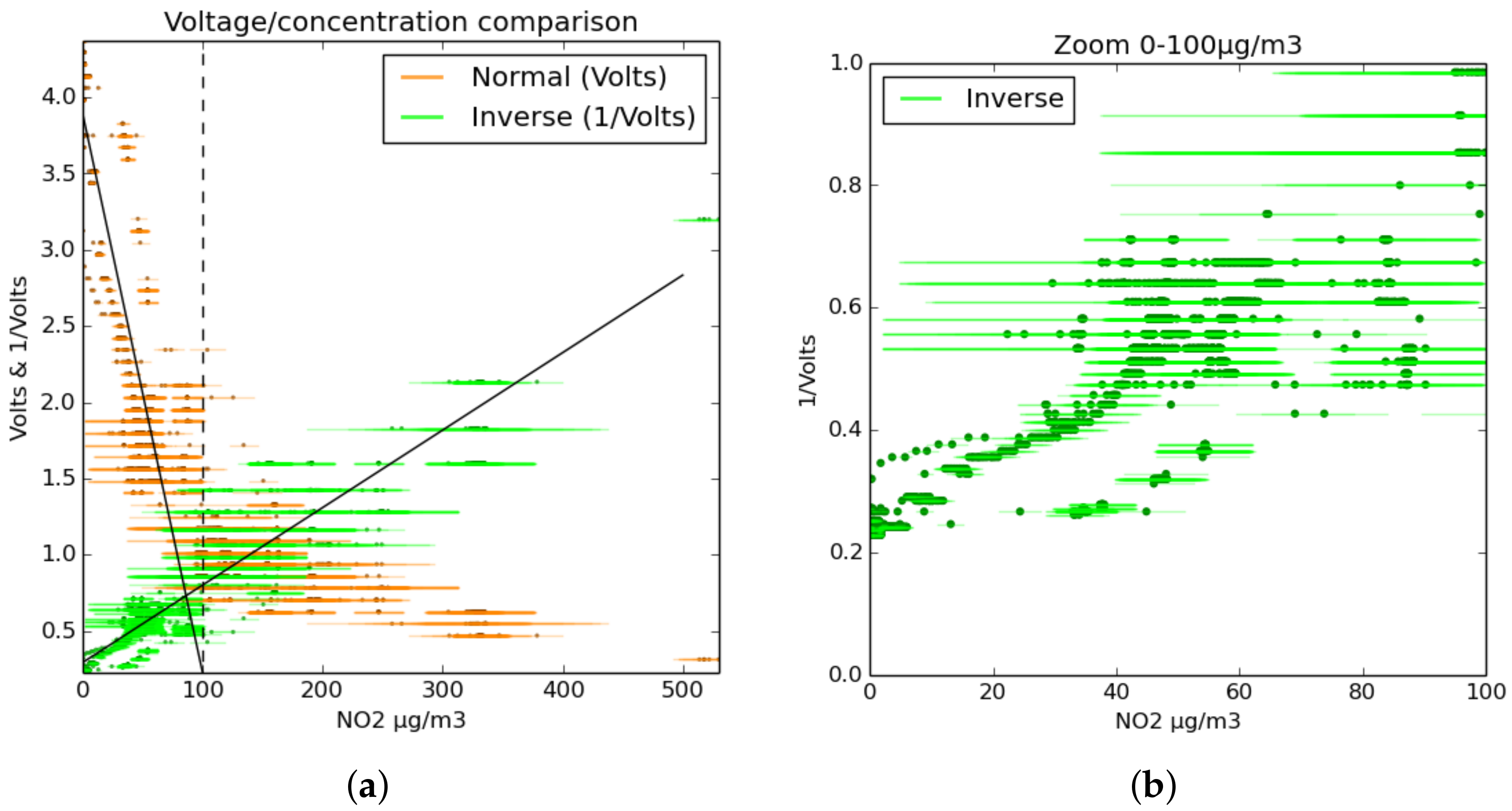
1.3. Theory of MOS Sensor Response
1.4. Warm-Up Time
1.5. Statistical Definitions
2. Materials and Methods
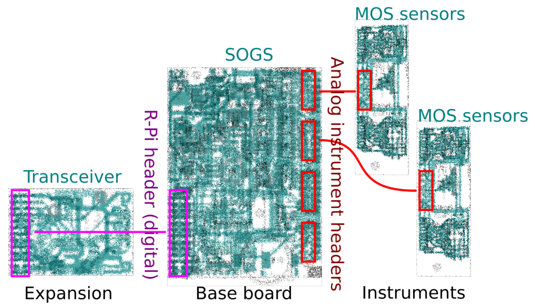
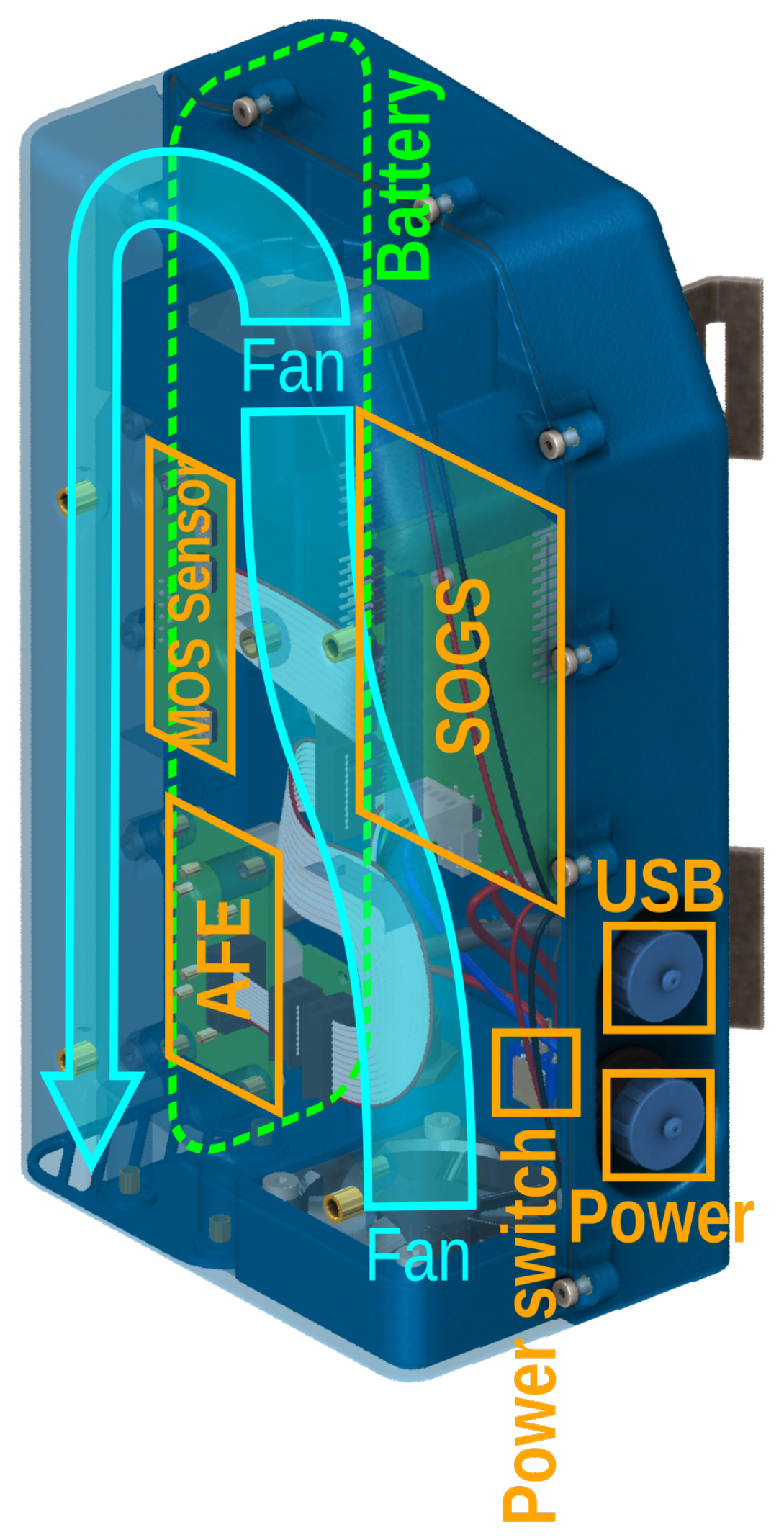
2.1. Instrument Architecture
2.2. Zephyr
3. Results and Discussion
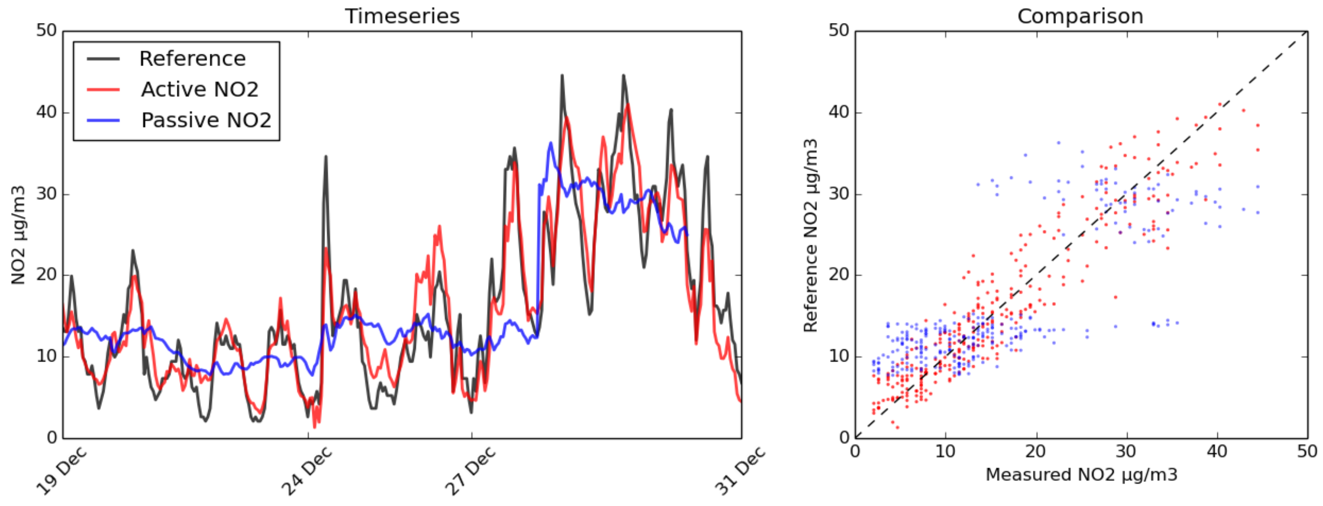
3.1. Comparison with BBCEAS
3.2. Calibration
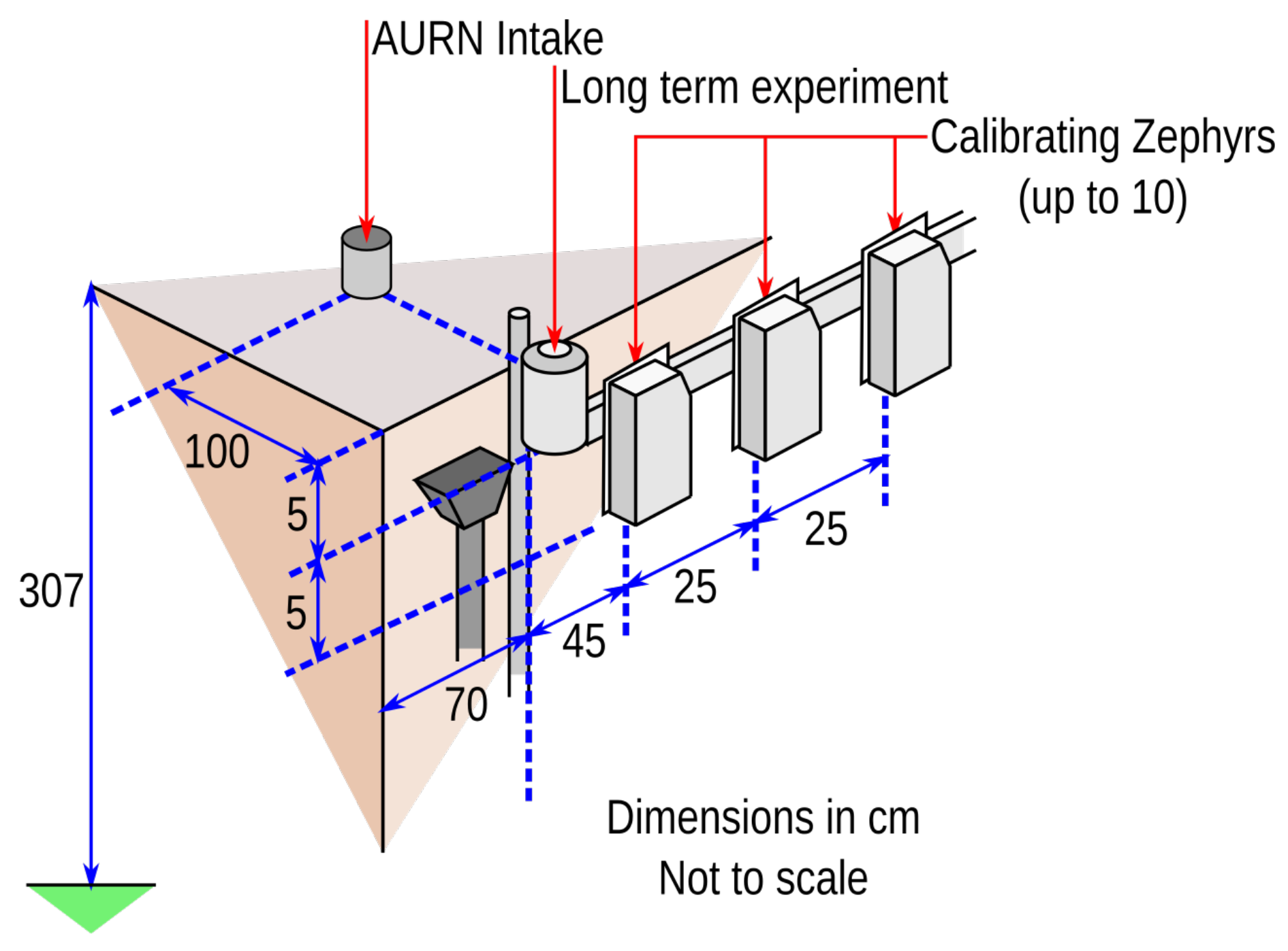
- The AURN intake has an isokinetic pump that draws air down to the chemiluminescence sensors operated on behalf of DEFRA.
- The second is on a long-term SOGS-based experiment using MOS sensors. This instrument uses an older casing for pollution observing devices, but identical MOS sensor boards to the most modern Zephyr designs. This device has been out on the AURN since December 2014.
- The third group of sensor intakes belongs to MOS sensors, which are mounted on plates along a horizontal crossbar. There are ten mounting points for these sensors, roughly 25 cm apart each.
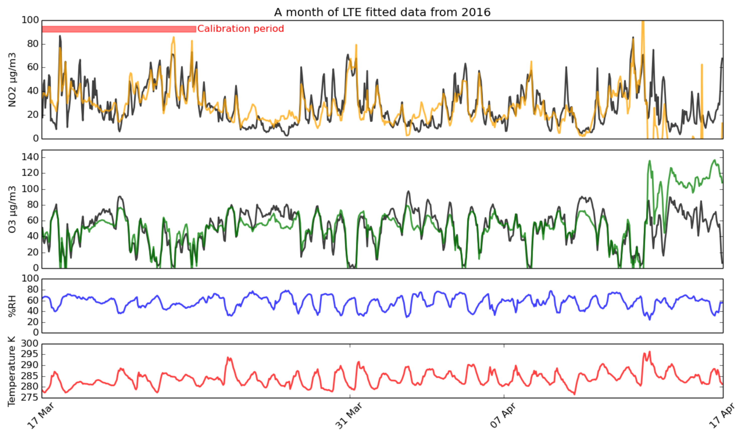
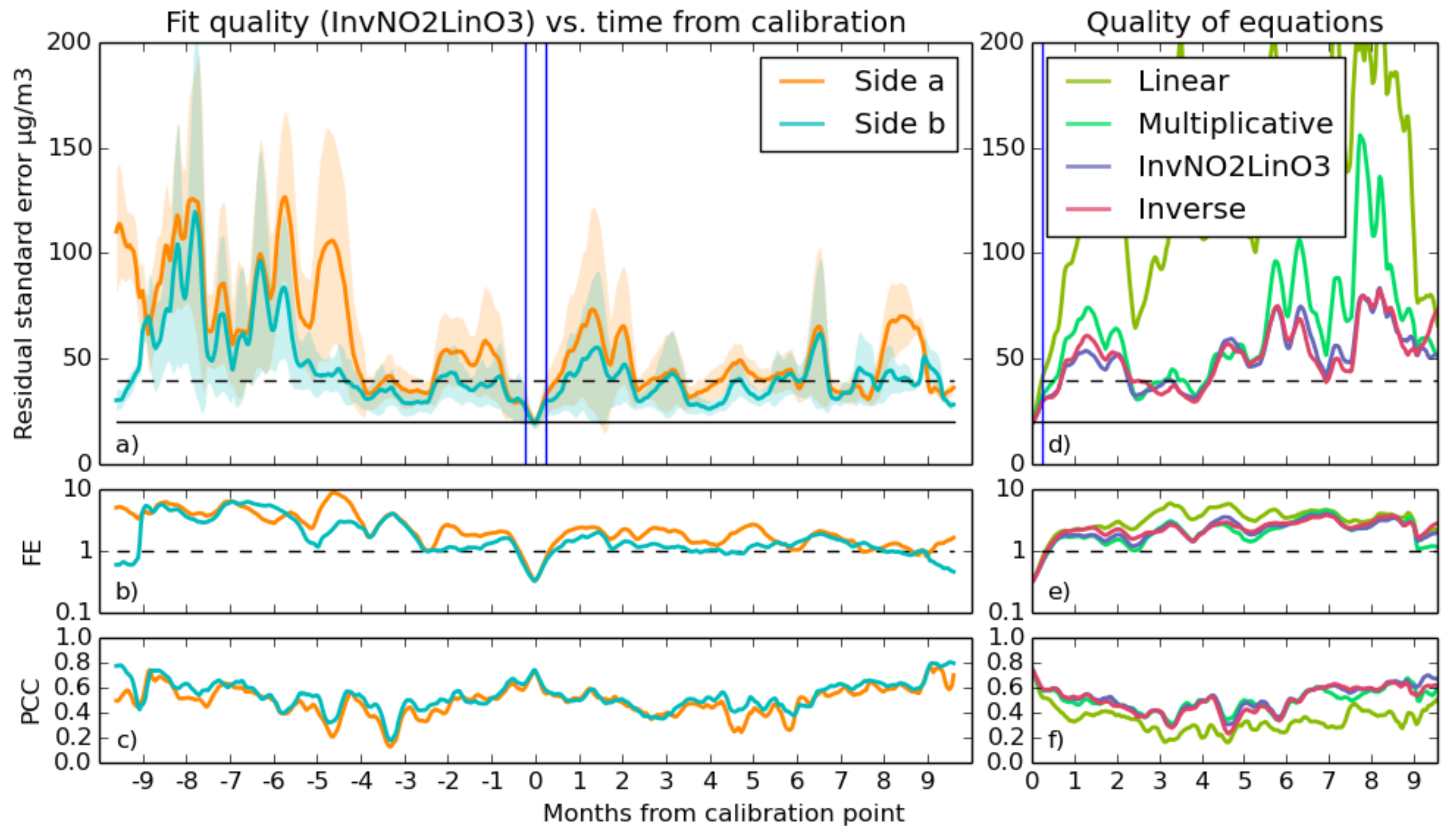
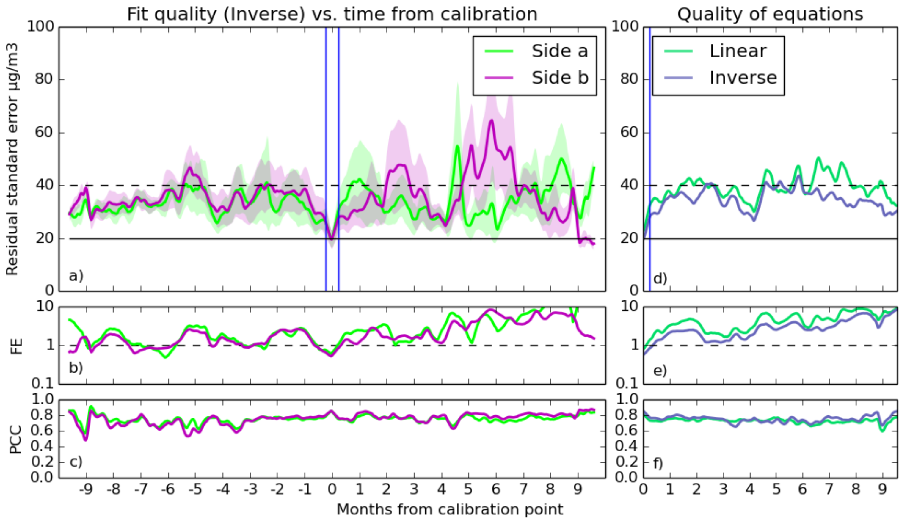
3.2.1. Long-Term Experiment and Calibration Equations
- Linear:This equation assumes that the influence of temperature and humidity is proportional to total sensor resistance and allows for ozone sensor cross-interference.
- Multiplicative linear:This equation uses product terms to factor in the effect that temperature and ozone interference has on the sensor’s performance. The use of the temperature term as a multiplicative factor with the voltage was suggested by the response of CO sensors to changing temperatures in Piedrahita et al. [30].
- Inverse:This modified equation uses inverse terms in an attempt to more accurately model the curve of the sensor’s response over a greater range.
- Inverse NO2, Linear O3 multiplicative:An alternative to the inverse equation that maintains linear terms on the ozone voltage is abbreviated as InvNO2LinO3.
- Linear:This simple equation keeps the multiplicative terms for temperature and humidity.
- Inverse:an ozone equation with inverted voltage terms.
- The AURN and MOS sensor time series was sliced into sections between six and seven days long when data were available, contracting to a minimum of six days where there were gaps in the data, at hourly offsets.
- A linear fit was taken using the calibration equation over every one of these periods, giving an array of fit coefficients.
- Each set of these coefficients was used to predict gas levels for the entire time series, producing an array of predicted time series.
- Using a similar moving window over each predicted data series, statistical functions measuring the goodness of fit were calculated. These functions are the Pearson correlation coefficient between prediction and reference (Equation (9)), residual standard error (Equation (7)) and residual fractional error (Equation (8)). Each application of this method to a prediction gives an error time series, which represents how good the fit is at a particular time. At the end of this process, there is one error time series for each prediction.
- The timestamps of the error time series were shifted so that they aligned over the week at which the calibration was taken. Thus, at time = zero, the standard error array for a particular time series gives the error over the same period at which the calibration that produced it took place.
- Finally, all of the error time series were split into day-lengths, and an average of all of them over each day was taken to give the statistical errors of the sensor’s prediction as a function of the time from the calibration. The standard error of the data in these day-long bins is a representation of the variation in quality of fits at predicting data at that particular time. The gaps in the original data are averaged over the entire length of this output, making it continuous.
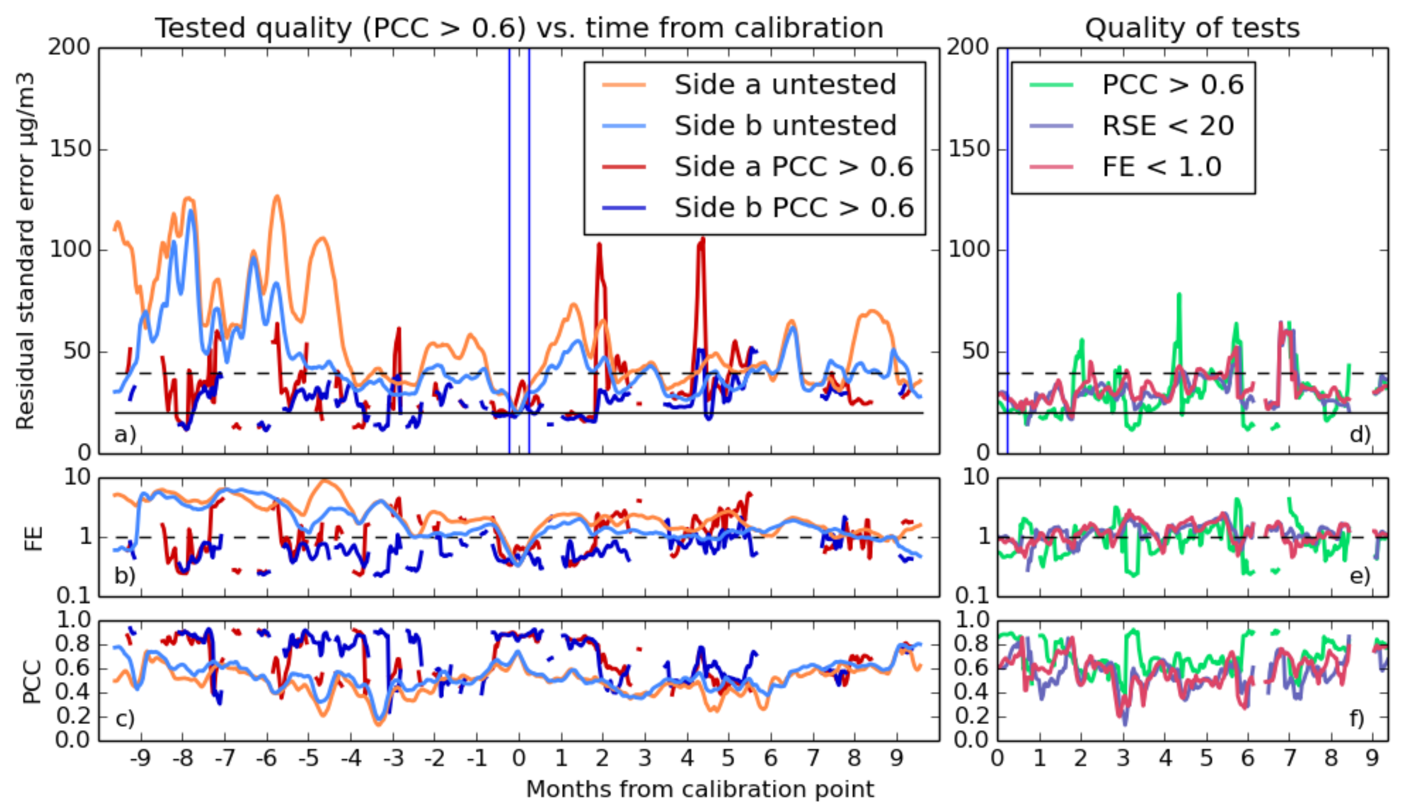
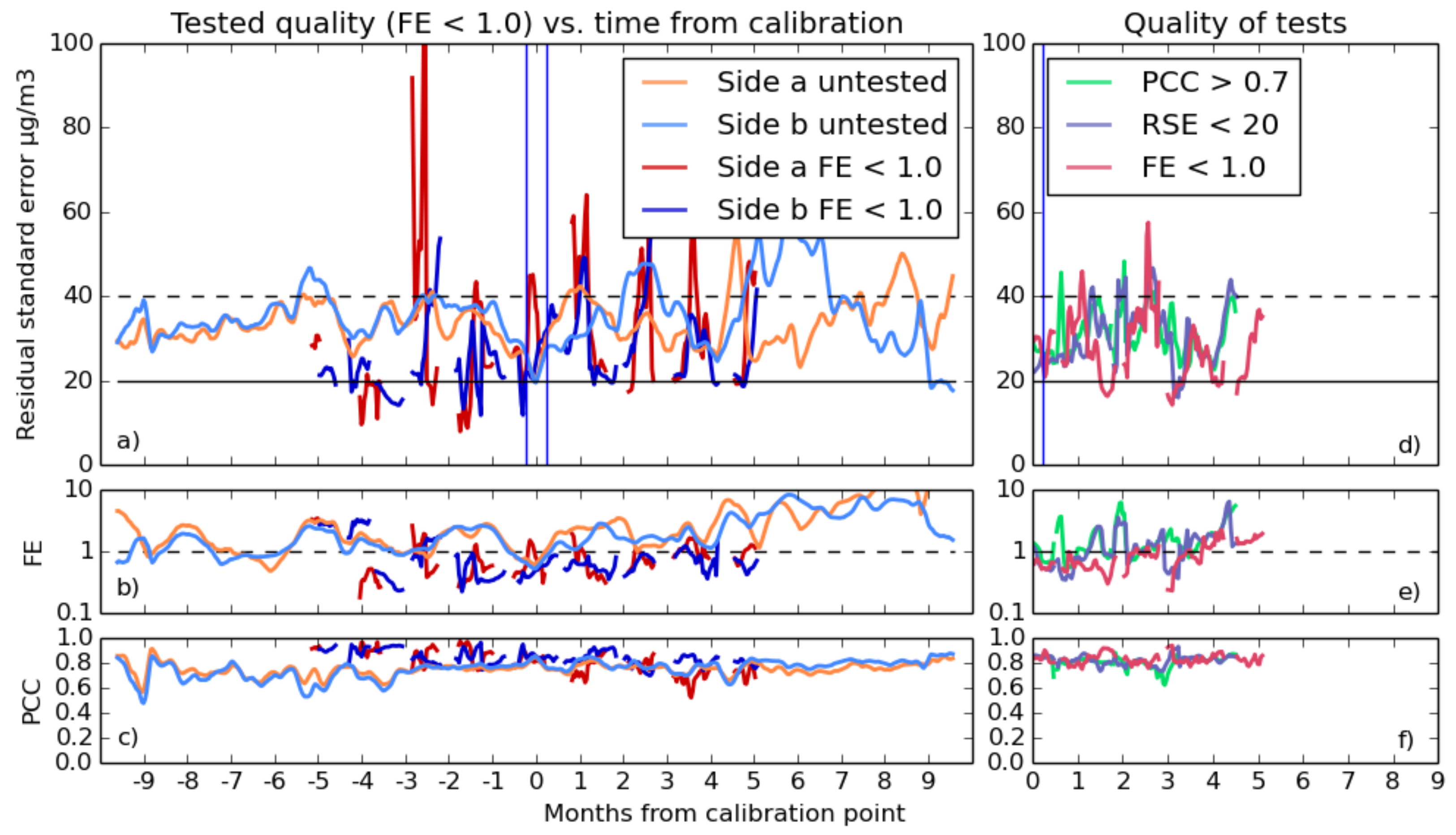
3.2.2. Selecting Good Fits
- With RSE, a fit qualifies if its standard error is below 20 , in line with the accuracy goals.
- For FE, the test is passed if the fractional error is below one. This is a fairly loose constraint, but during some calibrations, the predicted values, which are reasonable during the calibration period, start to deviate drastically during the validation period. This test will filter out those cases.
- There were several thresholds for correlation used, as the different gas fits typically were capable of differing levels of quality. Values of 0.6, 0.7 or 0.8 are all compared for both gases.
3.2.3. Calibration and Validation Times
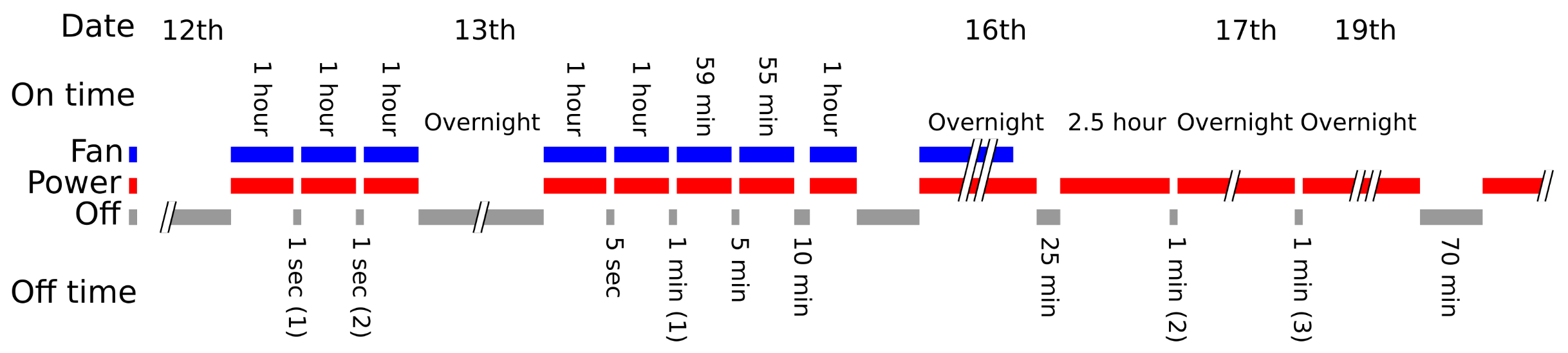
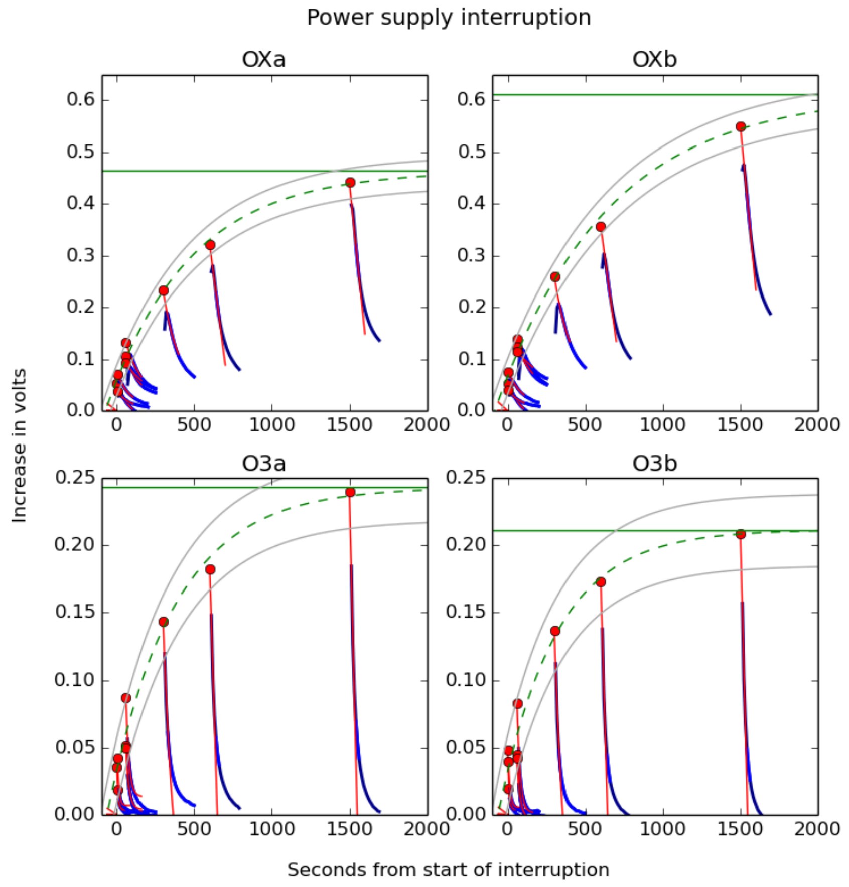
3.3. Warm-Up Time
3.3.1. Experimental Method
3.3.2. Discussion
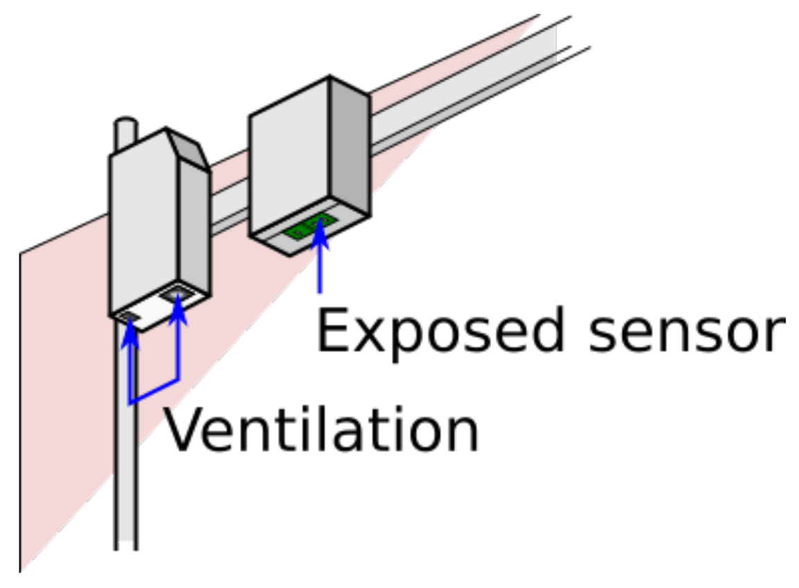
3.4. Airflow
Discussion
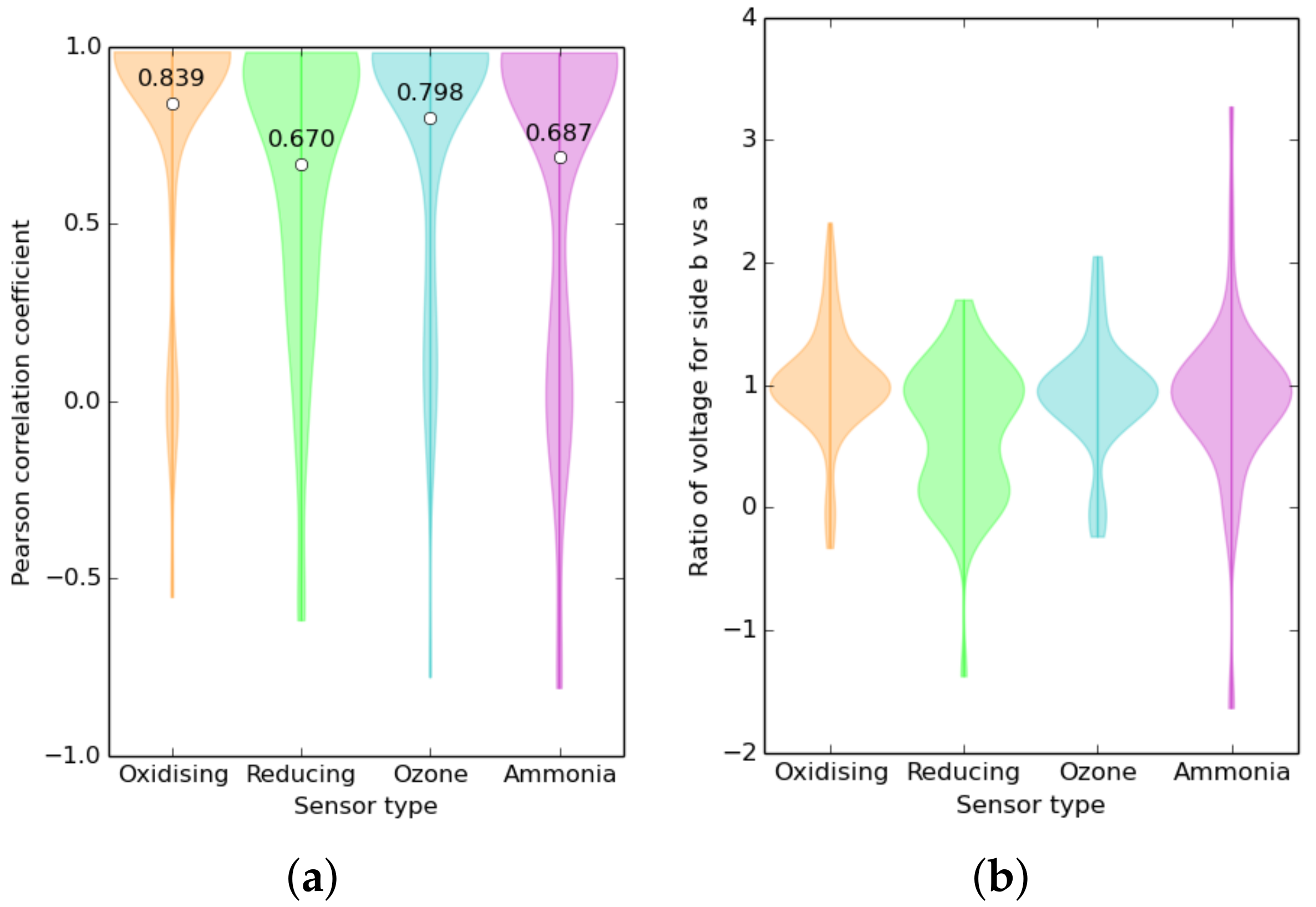
3.5. Variability between Sensors: Environment or Manufacturing?
4. Conclusions
Acknowledgments
Author Contributions
Conflicts of Interest
Abbreviations
| OMI | Ozone Monitoring Instrument |
| ANDI | Atmospheric Nitrogen Dioxide Imager |
| AURN | Automatic Urban/Rural Network |
| DEFRA | Department for the Environment, Food and Rural Affairs |
| MOS | Metal Oxide Semiconductor |
| LTE | Long-Term Experiment |
| FE | Fractional Error |
| RSE | Residual Standard Error |
| PCC | Pearson Correlation Coefficient |
| tFC | Time From Calibration |
| InvNO2LinO3 | Inverse NO2, Linear O3 equation |
References
- Gruber, N.; Galloway, J.N. An Earth-system perspective of the global nitrogen cycle. Nature 2008, 451, 293–296. [Google Scholar] [CrossRef] [PubMed]
- Zhiyong, W.; Xuemei, W.; Fei, C.; Turnipseed, A.A.; Guenther, A.B.; Dev, N.; Charusombat, U.; Beicheng, X.; Munger, J.W.; Alapaty, K. Evaluating the calculated dry deposition velocities of reactive nitrogen oxides and ozone from two community models over a temperate deciduous forest. Atmos. Environ. 2011, 45, 2663–2674. [Google Scholar]
- Rijnders, E.; Janssen, N.A.; Van Vliet, P.H.; Brunekreef, B. Personal and outdoor nitrogen dioxide concentrations in relation to degree of urbanization and traffic density. Int. J. Hydrogen Energy 2001, 109, 411. [Google Scholar]
- Erisman, J.W.; Grennfelt, P.; Sutton, M. Nitrogen emission and deposition: The European perspective. Sci. World J. 2001, 1, 879–896. [Google Scholar] [CrossRef] [PubMed]
- Hewitt, N. Spatial variations in nitrogen dioxide concentrations in an urban area. Atmos. Environ. B-URB 1991, 25, 429–434. [Google Scholar] [CrossRef]
- Briggs, D.J. The role of GIS: Coping with space (and time) in air pollution exposure assessment. J. Toxicol. Environ. Health 2005, 68, 1243–1261. [Google Scholar] [CrossRef] [PubMed]
- Yifang, Z.; Hinds, W.C.; Seongheon, K.; Si, S.; Sioutas, C. Study of ultrafine particles near a major highway with heavy-duty diesel traffic. Atmos. Environ. 2002, 36, 4323–4335. [Google Scholar]
- Levelt, P.F.; van den Oord, G.H.J.; Dobber, M.R.; Mälkki, A.; Visser, H.; de Vries, J.; Stammes, P.; Lundell, J.O.V.; Saari, H. The Ozone Monitoring Instrument. IEEE Trans. Geosci. Remote 2006, 44, 1093. [Google Scholar] [CrossRef]
- Lawrence, J.P.; Anand, J.S.; Vande Hey, J.D.; White, J.; Leigh, R.R.; Monks, P.S.; Leigh, R.J. High-resolution measurements from the airborne Atmospheric Nitrogen Dioxide Imager (ANDI). Atmos. Meas. Tech. 2015, 8, 4735–4754. [Google Scholar] [CrossRef]
- Model T200P Photolytic NO/NO2/NOX Analyser. Available online: http://www.et.co.uk/products/air-quality-monitoring/continuous-gas-analysers/no-no2-model-t200p-photolytic-nono2-nox-analyser (accessed on 6 May 2017).
- Kumar, P.; Morawska, L.; Martani, C.; Biskos, G.; Neophytou, M.; Di Sabatino, S.; Bell, M.; Norford, L.; Britter, R. The rise of low-cost sensing for manageing air pollution in cities. Environ. Int. 2015, 75, 199–205. [Google Scholar] [CrossRef] [PubMed]
- Palmes, E.D.; Gunnison, A.F.; DiMattio, J.; Tomczyk, C. Personal sampler for nitrogen dioxide. Am. Ind. Sci. Assoc. J. 1976, 37, 570–577. [Google Scholar] [CrossRef] [PubMed]
- Mead, M.I.; Popoola, O.A.M.; Stewart, G.B.; Landshoff, P.; Calleja, M.; Hayes, M.; Baldovi, J.J.; McLeod, M.W.; Hodgson, T.F.; Dicks, J.; et al. The use of electrochemical sensors for monitoring urban air quality in low-cost, high-density networks. Atmos. Environ. 2013, 70, 186–203. [Google Scholar] [CrossRef]
- Fine, G.F.; Cavanagh, L.M.; Afonja, A.; Binions, R. Metal oxide semi-conductor gas sensors in environmental monitoring. Sensors 2010, 10, 5469–5502. [Google Scholar] [CrossRef] [PubMed]
- Masson, N.; Piedrahita, R.; Hannigan, M. Approach for quantification of metal oxide type semiconductor gas sensors used for ambient air quality monitoring. Sens. Actuators B Chem. 2015, 208, 339–345. [Google Scholar] [CrossRef]
- Vezzoli, M.; Ponzoni, A.; Pardo, M.; Falasconi, M.; Faglia, G.; Sberveglieri, G. Exploratory data analysis for industrial safety application. Sens. Actuators B Chem. 2008, 131, 100–109. [Google Scholar] [CrossRef]
- Boon-Brett, L.; Bousek, J.; Moretto, P. Reliability of commercially available hydrogen sensors for detection of hydrogen at critical concentrations: Part II—Selected sensor test results. Int. J. Hydrogen Energy 2009, 34, 562–571. [Google Scholar] [CrossRef]
- Buttner, W.J.; Post, M.B.; Burgess, R.; Rivkin, C. An overview of hydrogen safety sensors and requirements. Int. J. Hydrogen Energy 2011, 36, 2462–2470. [Google Scholar] [CrossRef]
- Williams, D.E.; Salmond, J.; Fai, Y.; Jin, A.; Wright, B.; Wilson, J.; Henshaw, G.S.; Wells, D.B.; Ding, G.; Wagner, J.; et al. Development of low-cost ozone and nitrogen dioxide measurement instruments suitable for use in an air quality monitoring network. In Proceedings of the 2009 IEEE Sensors, Christchurch, New Zealand, 25–28 October 2009; pp. 1099–1104. [Google Scholar]
- Elmi, I.; Zampolli, S.; Cozzani, E.; Mancarella, F.; Cardinali, G.C. Development of ultra-low-power consumption MOX sensors with ppb-level VOC detection capabilities for emerging applications. Sens. Actuator Chem. 2008, 135, 342–351. [Google Scholar] [CrossRef]
- Zampolli, S.; Elmi, I.; Mancarella, F.; Betti, P.; Dalcanale, E.; Cardinali, G.C.; Severi, M. Real-time monitoring of sub-ppb concentrations of aromatic volatiles with a MEMS-enabled miniaturized gas-chromatograph. Sens. Actuator Chem. 2009, 141, 322–328. [Google Scholar] [CrossRef]
- Williams, D.E.; Aliwell, S.R.; Pratt, K.F.E.; Caruana, D.J.; Jones, R.L.; Cox, R.A.; Hansford, G.M.; Halsall, J. Modelling the response of a tungsten oxide semiconductor as a gas sensor for the measurement of ozone. Meas. Sci. Technol. 2002, 13, 923. [Google Scholar] [CrossRef]
- Bicelli, S.; Depari, A.; Faglia, G.; Flammini, A.; Fort, A.; Mugnaini, M.; Ponzoni, A.; Vignoli, V.; Rocchi, S. Model and experimental characterization of the dynamic behavior of low-power carbon monoxide MOX sensors operated with pulsed temperature profiles. Meas. Sci. Technol. 2009, 58, 1324–1332. [Google Scholar] [CrossRef]
- Burresi, A.; Fort, A.; Rocchi, S.; Serrano, B.; Ulivieri, N.; Vignoli, V. Dynamic CO recognition in presence of interfering gases by using one MOX sensor and a selected temperature profile. Sens. Actuator Chem. 2005, 106, 40–43. [Google Scholar] [CrossRef]
- Ionescu, R.; Vancu, A.; Tomescu, A. Time-dependent humidity calibration for drift corrections in electronic noses equipped with SnO2 gas sensors. Sens. Actuators B Chem. 2000, 69, 283–286. [Google Scholar] [CrossRef]
- Sohn, J.H.; Atzeni, M.; Zeller, L.; Pioggia, G. Characterisation of humidity dependence of a metal oxide semiconductor sensor array using partial least squares. Sens. Actuators B Chem. 2008, 131, 230–235. [Google Scholar] [CrossRef]
- Romain, A.-C.; Nicolas, J.; Andre, P. In situ measurement of olfactive pollution with inorganic semiconductors: Limitations due to humidity and temperature influence. Semin. Food Anal. 1997, 2, 283–296. [Google Scholar]
- Lei, Z.; Feng-Chun, T.; Xiong-Wei, P.; Xin, Y. A rapid discreteness correction scheme for reproducibility enhancement among a batch of MOS gas sensors. Sens. Actuators A Phys. 2014, 205, 170–176. [Google Scholar]
- Romain, A.-C.; Nicolas, J. Long term stability of metal oxide-based gas sensors for e-nose environmental applications: An overview. Sens. Actuators B Chem. 2010, 146, 502–506. [Google Scholar] [CrossRef]
- Piedrahita, R.; Xiang, Y.; Masson, N.; Ortega, J.; Collier, A.; Jiang, Y.; Li, K.; Dick, R.; Lv, Q.; Hannigan, M.; et al. The next generation of low-cost personal air quality sensors for quantitative exposure monitoring. Atmos. Meas. Tech. 2014, 7, 3325–3336. [Google Scholar] [CrossRef]
- Directive 2008/50/EC of the European Parliament. Off. J. Eur. Union 2008, 152, 1–44. Available online: http://ec.europa.eu/environment/air/quality/standards.htm (accessed on 18 July 2017).
- Vitz, E.D.; Chan, H. LIMSport VII. Semiconductor gas sensors as GC detectors and “breathalyzers”. J. Chem. Educ. 1995, 72, 920. [Google Scholar] [CrossRef]
- Meixner, H.; Lampe, U. Metal oxide sensors. Sens. Actuators B Chem. 1996, 33, 198–202. [Google Scholar] [CrossRef]
- Naisbitt, S.C.; Pratt, K.F.E.; Williams, D.E.; Parkin, I.P. A microstructural model of semiconducting gas sensor response: The effects of sintering temperature on the response of chromium titanate (CTO) to carbon monoxide. Sens. Actuators B Chem. 2006, 114, 969–977. [Google Scholar] [CrossRef]
- Scott, B. Utilizing Portable Air Quality Monitors to Assess the Patterns of Ozone along the Northern Front Range of Colorado. SOARS 2014. Available online: https://pdfs.semanticscholar.org/5eb7/4f0ae4ed93be65c1e3048b8dc4684fce8617.pdf (accessed on 13 July 2017).
- Spinelle, L.; Gerboles, M.; Villani, M.G.; Aleixandre, M.; Bonavitacola, F. Field calibration of a cluster of low-cost available sensors for air quality monitoring. Part A: Ozone and nitrogen dioxide. Sens. Actuators B Chem. 2015, 215, 249–257. [Google Scholar] [CrossRef]
- MICS 4514 Datasheet (0278 Revision 15). Available online: https://www.sgxsensortech.com/content/uploads/2014/08/0278_Datasheet-MiCS-4514.pdf (accessed on 13 July 2017).


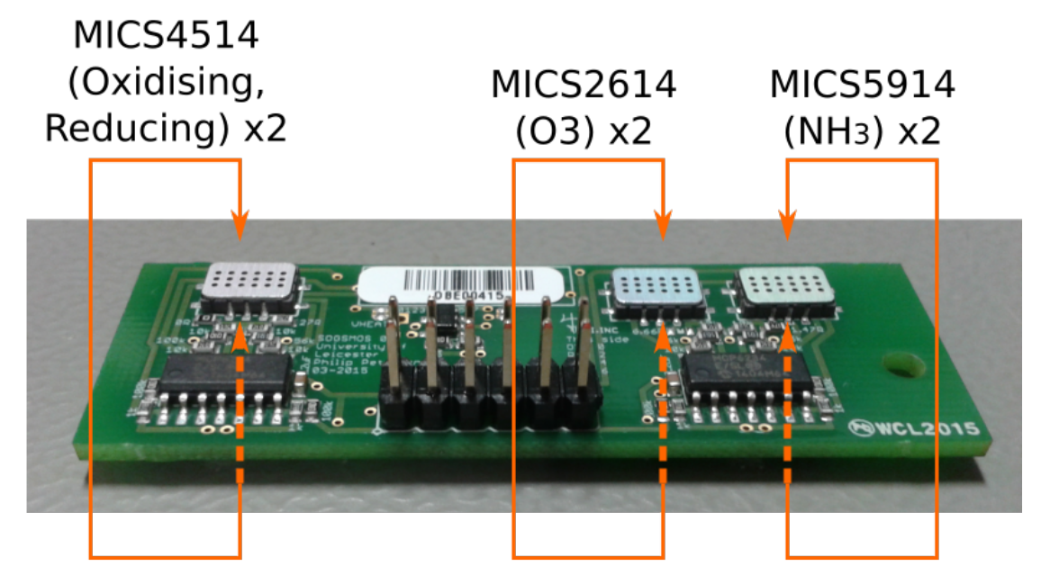
| Parameter Measured | Sensor Part Number | Method of Detection | Gas Detected and Detection limits | Resolution |
|---|---|---|---|---|
| Reducing Gases | SGX Sensortech MICS-4514 | redox reaction | CO: 1–1000 ppm | N/A |
| NH3: 1–500 ppm | ||||
| C2H5OH: 10–500 ppm | ||||
| H2: 1–1000 ppm | ||||
| CH4: >1000 ppm | ||||
| Oxidising Gases | SGX Sensortech | redox reaction | NO2: 0.05–10 ppm | N/A |
| MICS-4514 | H2: 1–1000 ppm | |||
| O3 | SGX Sensortech | redox reaction | 10–1000 ppb | N/A |
| MICS-2614 | ||||
| NH3 | SGX Sensortech MICS-5914 | redox reaction | NH3: 1-500 ppm | N/A |
| C2H5OH: 10–500 ppm | ||||
| H2: 1–1000 ppm | ||||
| C3H8: >1000 ppm | ||||
| C2H8(CH4)2: >1000 ppm | ||||
| Temperature and Relative Humidity | GE Measurement and Control CC2D25 | Polyimide capacitance | Temperature: −40–125 °C Relative humidity: 0–100% | ±0.3 °C 2% |
| Gas | Metric | Side | Untested | PCC > 0.6 | PCC > 0.7 | PCC > 0.8 | RSE < 20 | FE < 1.0 | ||||||
|---|---|---|---|---|---|---|---|---|---|---|---|---|---|---|
| Mean | 2SD | Mean | 2SD | Mean | 2SD | Mean | 2SD | Mean | 2SD | Mean | 2SD | |||
| NO2 | RSE | a | 57.2 | 50.1 | 32.5 | 33.5 | 24.7 | 13.1 | 20.3 | 9.3 | 34.5 | 31.1 | 35.0 | 29.6 |
| b | 44.2 | 33.7 | 25.7 | 16.5 | 22.2 | 11.4 | 20.4 | 10.1 | 29.0 | 16.3 | 28.4 | 14.3 | ||
| FE | a | 2.60 | 3.28 | 1.38 | 2.20 | 0.77 | 1.05 | 0.63 | 1.05 | 1.47 | 1.86 | 1.51 | 1.91 | |
| b | 1.98 | 2.94 | 0.67 | 0.73 | 0.59 | 0.69 | 0.44 | 0.27 | 1.01 | 1.08 | 0.94 | 1.07 | ||
| PCC | a | 0.49 | 0.23 | 0.68 | 0.33 | 0.73 | 0.37 | 0.87 | 0.09 | 0.57 | 0.33 | 0.57 | 0.33 | |
| b | 0.54 | 0.22 | 0.71 | 0.35 | 0.72 | 0.38 | 0.85 | 0.14 | 0.54 | 0.46 | 0.60 | 0.35 | ||
| Used | a | 100% | 54% | 15% | 12% | 75% | 82% | |||||||
| b | 100% | 60% | 24% | 11% | 74% | 74% | ||||||||
| O3 | RSE | a | 33.6 | 10.9 | 34.4 | 32.4 | 32.6 | 29.0 | 35.4 | 34.6 | 32.6 | 29.4 | 31.6 | 31.9 |
| b | 35.5 | 15.8 | 32.4 | 22.4 | 30.3 | 26.8 | 27.1 | 17.5 | 31.0 | 28.8 | 26.4 | 18.3 | ||
| FE | a | 3.62 | 8.79 | 3.09 | 13.5 | 3.31 | 15.3 | 3.42 | 14.7 | 3.12 | 14.8 | 0.89 | 1.27 | |
| b | 2.37 | 3.67 | 2.01 | 3.53 | 2.13 | 3.92 | 1.52 | 3.40 | 1.94 | 4.10 | 0.91 | 1.52 | ||
| PCC | a | 0.75 | 0.09 | 0.78 | 0.18 | 0.81 | 0.15 | 0.81 | 0.15 | 0.80 | 0.18 | 0.80 | 0.19 | |
| b | 0.75 | 0.14 | 0.81 | 0.14 | 0.82 | 0.14 | 0.84 | 0.11 | 0.83 | 0.12 | 0.85 | 0.12 | ||
| Used | a | 100% | 79% | 81% | 58% | 75% | 29% | |||||||
| b | 100% | 82% | 78% | 56% | 75% | 42% | ||||||||
| Gas | Metric | Side | Untested | PCC > 0.6 | PCC > 0.7 | PCC > 0.8 | RSE < 20 | FE < 1.0 | ||||||
|---|---|---|---|---|---|---|---|---|---|---|---|---|---|---|
| Mean | 2SD | Mean | 2SD | Mean | 2SD | Mean | 2SD | Mean | 2SD | Mean | 2SD | |||
| NO2 | RSE | a | 37.5 | 22.6 | 24.4 | 9.69 | 20.5 | 6.37 | 20.0 | 5.43 | 28.9 | 12.1 | 28.5 | 10.1 |
| b | 32.6 | 14.0 | 19.9 | 5.09 | 19.3 | 7.37 | 20.3 | 4.31 | 23.4 | 8.70 | 22.7 | 7.77 | ||
| FE | a | 1.39 | 1.34 | 0.80 | 1.35 | 0.49 | 0.36 | 0.50 | 0.38 | 1.16 | 1.03 | 0.99 | 0.82 | |
| b | 1.06 | 0.88 | 0.66 | 1.01 | 0.41 | 0.21 | 0.46 | 0.28 | 0.62 | 0.44 | 0.59 | 0.39 | ||
| PCC | a | 0.57 | 0.13 | 0.85 | 0.14 | 0.89 | 0.04 | 0.89 | 0.02 | 0.64 | 0.28 | 0.64 | 0.30 | |
| b | 0.59 | 0.14 | 0.82 | 0.27 | 0.86 | 0.31 | 0.89 | 0.04 | 0.69 | 0.29 | 0.67 | 0.37 | ||
| Used | a | 100% | 58% | 50% | 50% | 75% | 83% | |||||||
| b | 100% | 77% | 58% | 45% | 87% | 85% | ||||||||
| O3 | RSE | a | 30.5 | 12.8 | 28.9 | 16.6 | 27.0 | 10.9 | 27.9 | 17.0 | 23.9 | 7.64 | 33.3 | 22.1 |
| b | 28.4 | 8.21 | 29.8 | 17.3 | 27.7 | 18.8 | 25.4 | 13.0 | 25.4 | 9.53 | 26.8 | 12.0 | ||
| FE | a | 1.41 | 1.26 | 0.81 | 1.11 | 0.83 | 0.91 | 1.28 | 1.83 | 0.76 | 0.83 | 0.80 | 0.85 | |
| b | 1.04 | 0.77 | 1.21 | 2.15 | 1.46 | 3.13 | 0.81 | 1.07 | 0.53 | 0.33 | 0.53 | 0.32 | ||
| PCC | a | 0.77 | 0.07 | 0.83 | 0.12 | 0.82 | 0.12 | 0.82 | 0.14 | 0.84 | 0.10 | 0.80 | 0.12 | |
| b | 0.78 | 0.06 | 0.81 | 0.15 | 0.82 | 0.20 | 0.84 | 0.10 | 0.83 | 0.08 | 0.84 | 0.06 | ||
| Used | a | 100% | 90% | 88% | 83% | 73% | 50% | |||||||
| b | 100% | 91% | 77% | 75% | 93% | 80% | ||||||||
© 2017 by the authors. Licensee MDPI, Basel, Switzerland. This article is an open access article distributed under the terms and conditions of the Creative Commons Attribution (CC BY) license (http://creativecommons.org/licenses/by/4.0/).
Share and Cite
Peterson, P.J.D.; Aujla, A.; Grant, K.H.; Brundle, A.G.; Thompson, M.R.; Vande Hey, J.; Leigh, R.J. Practical Use of Metal Oxide Semiconductor Gas Sensors for Measuring Nitrogen Dioxide and Ozone in Urban Environments. Sensors 2017, 17, 1653. https://doi.org/10.3390/s17071653
Peterson PJD, Aujla A, Grant KH, Brundle AG, Thompson MR, Vande Hey J, Leigh RJ. Practical Use of Metal Oxide Semiconductor Gas Sensors for Measuring Nitrogen Dioxide and Ozone in Urban Environments. Sensors. 2017; 17(7):1653. https://doi.org/10.3390/s17071653
Chicago/Turabian StylePeterson, Philip J. D., Amrita Aujla, Kirsty H. Grant, Alex G. Brundle, Martin R. Thompson, Josh Vande Hey, and Roland J. Leigh. 2017. "Practical Use of Metal Oxide Semiconductor Gas Sensors for Measuring Nitrogen Dioxide and Ozone in Urban Environments" Sensors 17, no. 7: 1653. https://doi.org/10.3390/s17071653
APA StylePeterson, P. J. D., Aujla, A., Grant, K. H., Brundle, A. G., Thompson, M. R., Vande Hey, J., & Leigh, R. J. (2017). Practical Use of Metal Oxide Semiconductor Gas Sensors for Measuring Nitrogen Dioxide and Ozone in Urban Environments. Sensors, 17(7), 1653. https://doi.org/10.3390/s17071653