State Estimation Using Dependent Evidence Fusion: Application to Acoustic Resonance-Based Liquid Level Measurement


Abstract
:1. Introduction
2. Foundations of Dempster-Shafer (DS) Evidence Theory
2.1. Basic Concepts in DS Evidence Theory
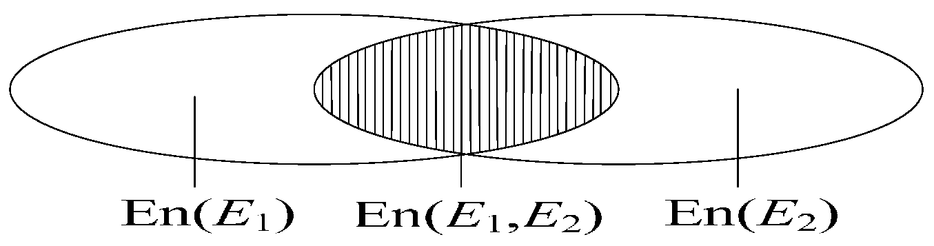
2.2. The Degree of Dependence and the Combination of Dependent Evidence
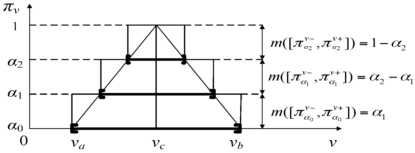
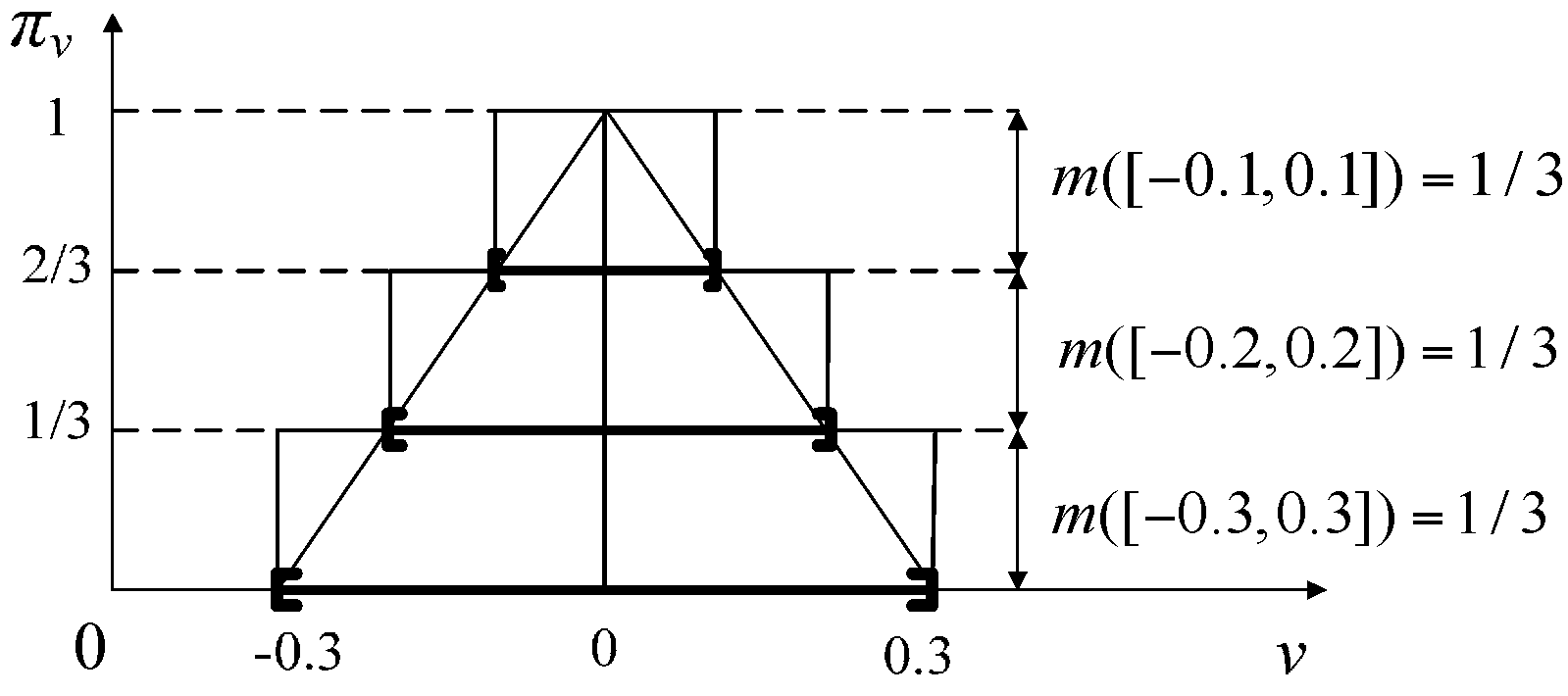
2.3. The Random Set Description of Evidence
2.3.1. Random Set and Random Relation
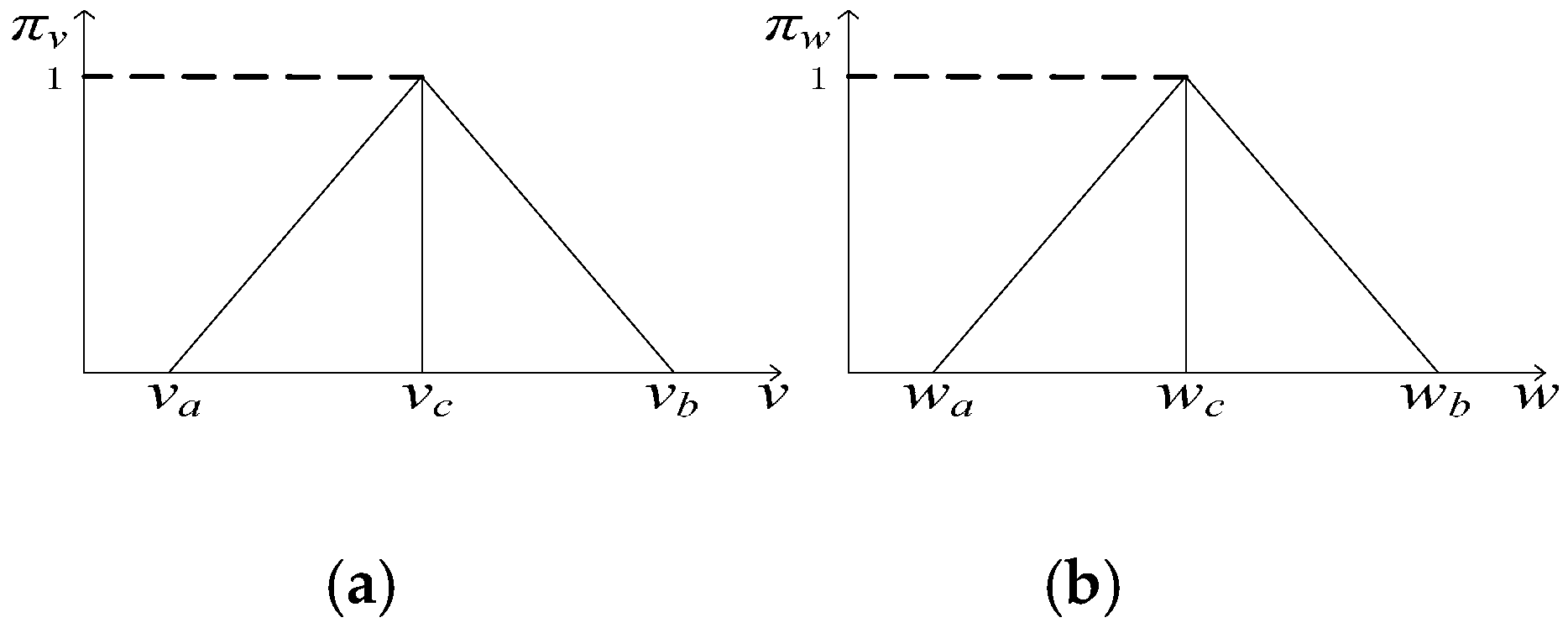
2.3.2. Extension Principles
3. State Estimation Based on Dependent Evidence Fusion
3.1. Dynamic System Model under Bounded Noises
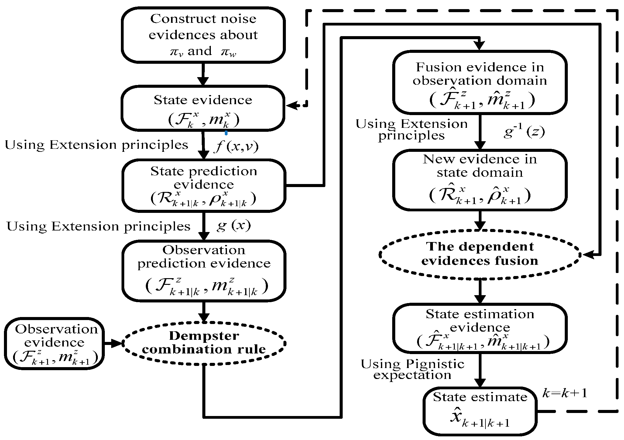
3.2. Recursive Algorithm of State Estimation Based on Extension Principles and Dependent Evidence Fusion
4. Application to Liquid Level Measurement
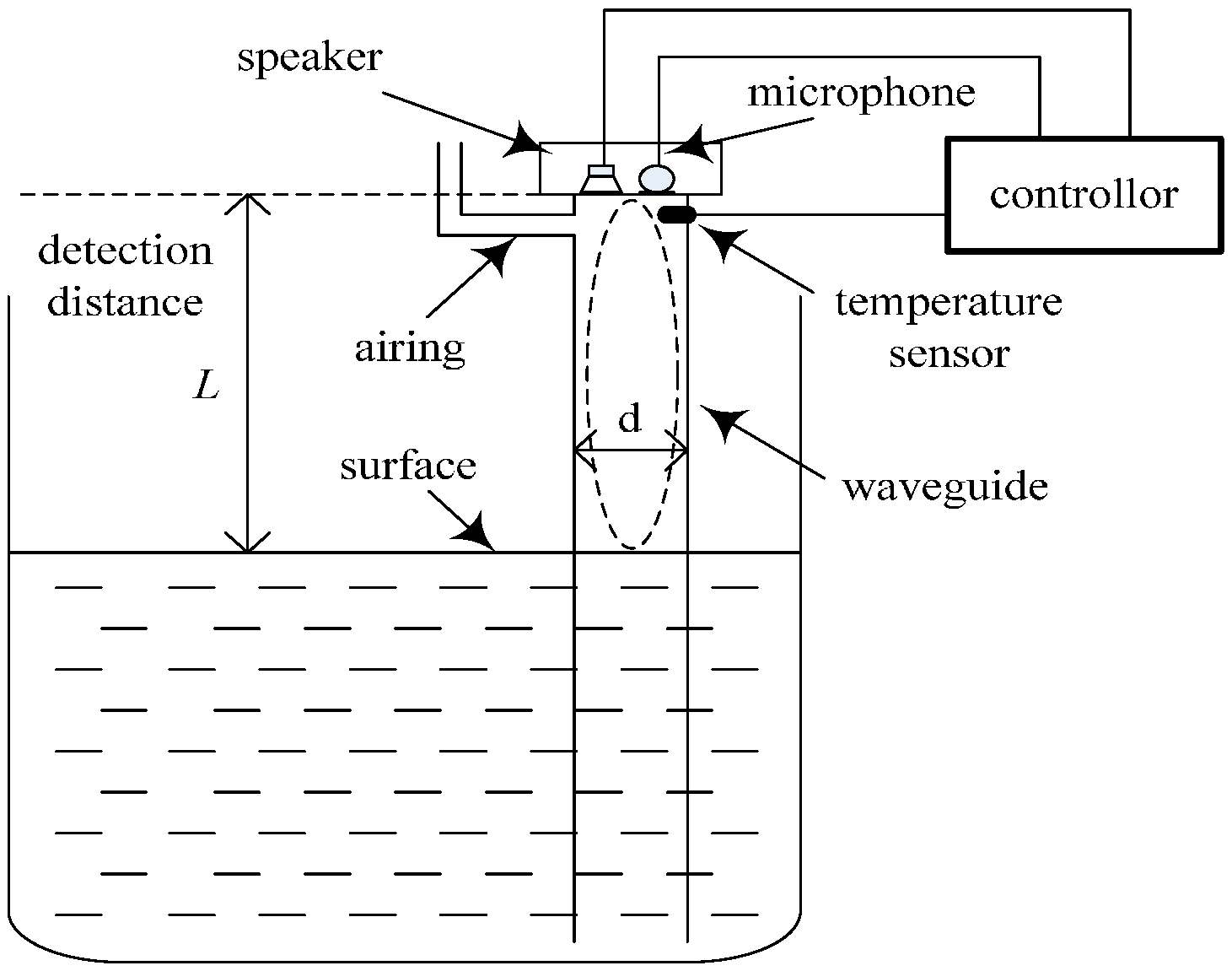
4.1. Acoustic Standing Wave Level Gauge
4.2. System Model
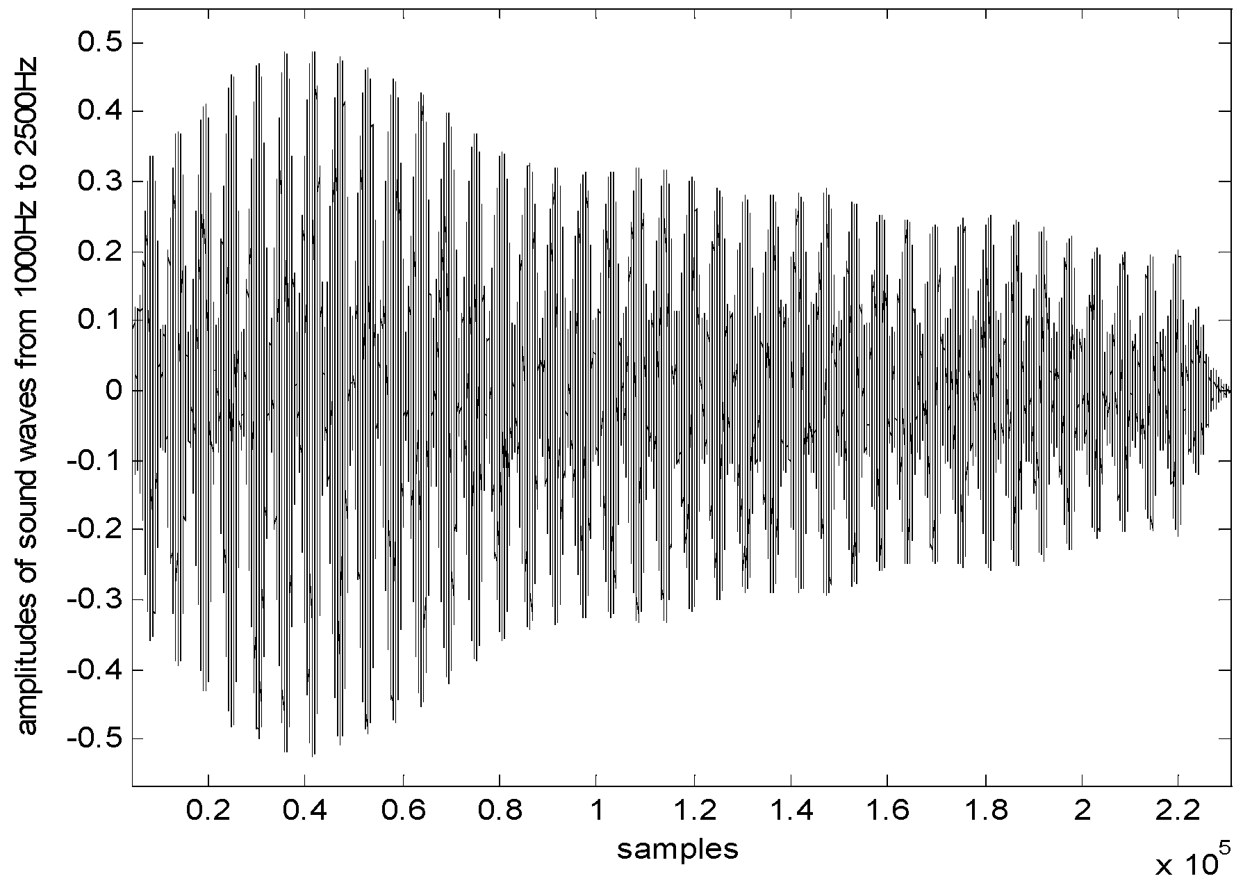
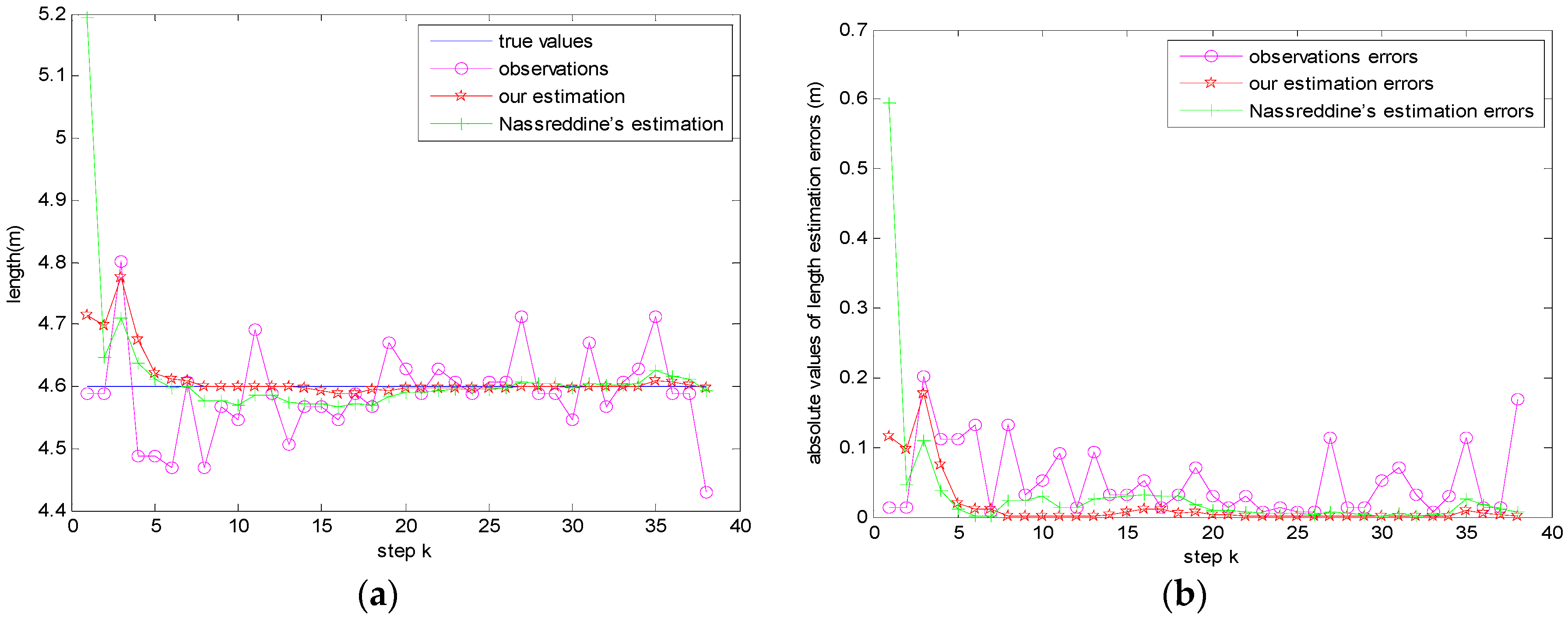
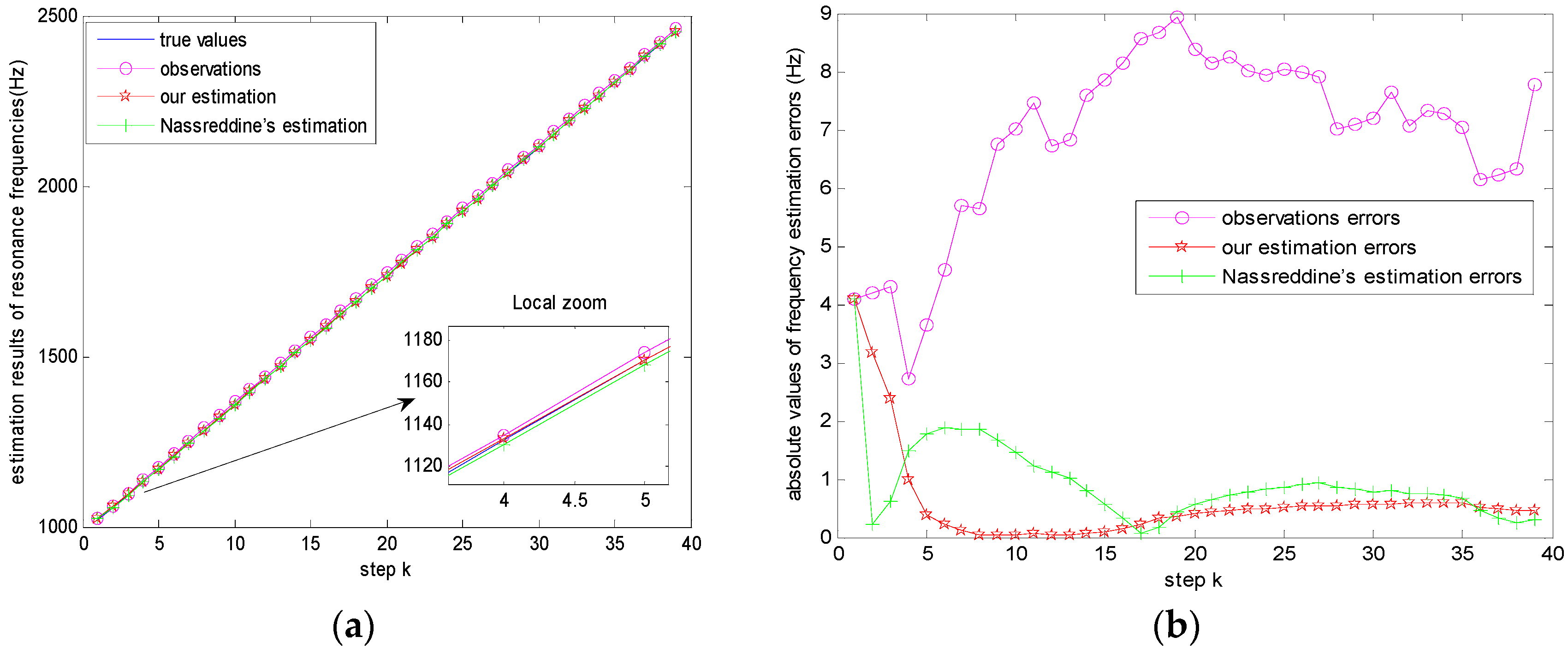
4.3. Liquid Level Estimation Tests
5. Conclusions
Acknowledgements
Author Contributions
Conflicts of Interest
Appendix A
References
- Song, Y.; Nuske, S.; Scherer, S. A Multi-Sensor Fusion MAV State Estimation from Long-Range Stereo, IMU, GPS and Barometric Sensors. Sensors 2017, 17, 11. [Google Scholar] [CrossRef] [PubMed]
- Gao, S.; Liu, Y.; Wang, J. The Joint Adaptive Kalman Filter (JAKF) for Vehicle Motion State Estimation. Sensors 2016, 16, 1103. [Google Scholar] [CrossRef] [PubMed]
- Kalman, R.E. A new approach to linear filtering and prediction problems. J. Basic Eng. 1960, 82, 35–45. [Google Scholar] [CrossRef]
- Kalman, R.E.; Bucy, R.S. New Results in Linear Filtering and Prediction Theory. J. Basic Eng. 1961, 83, 95–108. [Google Scholar] [CrossRef]
- Sunahara, Y.; Yamashita, K. An approximate method of state estimation for non-linear dynamical systems with state-dependent noise. Int. J. Control. 1970, 11, 957–972. [Google Scholar] [CrossRef]
- Gordon, N.J.; Salmond, D.J.; Smith, A.F.M. Novel approach to nonlinear/non-Gaussian Bayesian state estimation. Proc. Inst. Elect. Eng. F 1993, 140, 107–113. [Google Scholar] [CrossRef]
- Nassreddine, G.; Abdallah, F.; Denoux, T. State estimation using interval analysis and belief-function theory: application to dynamic vehicle localization. IEEE Trans. Syst. Man Cybern. B Cybern. 2010, 40, 1205–1218. [Google Scholar] [CrossRef] [PubMed]
- Brynjarsdóttir, J.; O’Hagan, A. Learning about physical parameters: The importance of model discrepancy. Inverse Prob. 2014, 30, 114007. [Google Scholar] [CrossRef]
- Bertsekas, D.P.; Rhodes, I.B. Recursive state estimation for a set-membership description of uncertainty. IEEE Trans. Autom. Control. 1971, 16, 117–128. [Google Scholar] [CrossRef]
- Maksarov, D.; Norton, J.P. State bounding with ellipsoidal set description of the uncertainty. Int. J. Control. 1996, 65, 847–866. [Google Scholar] [CrossRef]
- Servi, L.; Ho, Y. Recursive estimation in the presence of uniformly distributed measurement noise. IEEE Trans. Autom. Control 1981, 26, 563–565. [Google Scholar] [CrossRef]
- Gning, A.; Bonnifait, P. Constraints propagation techniques on intervals for a guaranteed localization using redundant data. Automatica 2006, 42, 1167–1175. [Google Scholar] [CrossRef]
- Khemane, F.; Abbas-Turki, M.; Durieu, C.; Raynaud, H.F.; Conan, J.M. Bounded-error state and parameter estimation of tip-tilt disturbances in adaptive optics systems. Int. J. Adapt Control Signal Process. 2014, 28, 1081–1093. [Google Scholar] [CrossRef]
- Jaulin, L. Range-only slam with occupancy maps: A set-membership approach. IEEE Trans. Robot 2011, 27, 1004–1010. [Google Scholar] [CrossRef]
- Dempster, A.P. Upper and lower probabilities induced by a multivalued mapping. Ann. Math. Stat. 1967, 38, 325–339. [Google Scholar] [CrossRef]
- Shafer, G. A Mathematical Theory of Evidence; Princeton University Press: Princeton, NJ, USA, 1976. [Google Scholar]
- Wu, Y.; Yang, J.; Liu, K.; Liu, L. On the evidence inference theory. Inform Sci. 1996, 89, 245–260. [Google Scholar] [CrossRef]
- Dubois, D.; Prade, H. Random sets and fuzzy interval analysis. Fuzzy Sets Syst. 1991, 42, 87–101. [Google Scholar] [CrossRef]
- Xu, X.; Zhou, D.; Ji, Y.; Wen, C. Approximating Probability Distribution of Circuit Performance Function for Parametric Yield Estimation Using Transferable Belief Model. Sci. Chin. Inf. Sci. 2013, 56, 50–69. [Google Scholar] [CrossRef]
- Goodman, I.R.; Mahler, R.P.S.; Nguyen, H.T. Mathematics of Data Fusion; Springer: Houten, The Netherlands, 1997. [Google Scholar]
- Jaulin, L.; Kieffer, M.; Didrit, O.; Walter, E. Applied Interval Analysis; Springer: London, UK, 2001. [Google Scholar]
- Dong, W.; Shah, H.C. Vertex method for computing functions of fuzzy variables. Fuzzy Sets Syst. 1987, 42, 65–78. [Google Scholar] [CrossRef]
- Smets, P. Belief functions on real numbers. Int. J. Approx. Reason. 2005, 40, 181–223. [Google Scholar] [CrossRef]
- Kazys, R.; Sliteris, R.; Rekuviene, R. Ultrasonic technique for density measurement of liquids in extreme conditions. Sensors 2015, 15, 19393–19415. [Google Scholar] [CrossRef] [PubMed]
- Donlagić, D.; Kumperščak, V.; Završnik, M. Low-frequency acoustic resonance level gauge. Sens. Actuators A Phys. 1996, 57, 209–215. [Google Scholar] [CrossRef]
- Donlagić, D.; Zavrsnik, M.; Sirotic, I. The use of one-dimensional acoustical gas resonator for fluid level measurements. IEEE Trans. Instrum Meas. 2000, 49, 1095–1100. [Google Scholar] [CrossRef]
- Xu, X.B.; Zhang, Z.; Zheng, J. State Estimation Method Based on Evidential Reasoning Rule. In Proceedings of the 2015 IEEE Advanced Information Technology, Electronic and Automation Control Conference (IAEAC), Chongqing, China, 19–20 December 2015. [Google Scholar]
- Xu, X.B.; Zhao, C.P.; Xia, B.D.; Wang, Z.; Wen, C.L. A fluid level measurement method based on acoustical resonance in a special frequency range. Acta Metroa Sin. 2011, 32, 53–57. [Google Scholar]


| [−0.1, 0.1] | [−0.2, 0.2] | [−0.3, 0.3] | [−10, 10] | |
| 0.3167 | 0.3167 | 0.3167 | 0.05 |
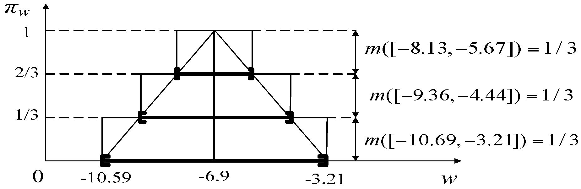
| [−8.13, −5.67] | [−9.36, −4.44] | [−10.59, −3.21] | [−129.7, 115.7] | |
| 0.3167 | 0.3167 | 0.3167 | 0.05 |
| No | True L (m) | T (°C) | Runtime (s) | Mean Error (m) | No | True L (m) | T (°C) | Runtime (s) | Mean Error (m) |
|---|---|---|---|---|---|---|---|---|---|
| 1 | 1.3 | 27 | 1.81 | 0.0126 | 6 | 5.6 | 26.5 | 20.11 | 0.018 |
| 0.88 | 0.016 | 4.81 | 0.0374 | ||||||
| - | 0.238 | - | 0.0661 | ||||||
| 2 | 2.1 | 26.5 | 2.49 | 0.0254 | 7 | 6.6 | 26.5 | 23.57 | 0.0238 |
| 1.33 | 0.0364 | 5.61 | 0.0436 | ||||||
| - | 0.0441 | - | 0.088 | ||||||
| 3 | 2.6 | 26.5 | 7.81 | 0.0144 | 8 | 7.6 | 26.5 | 27.94 | 0.0299 |
| 2.05 | 0.0297 | 6.77 | 0.0530 | ||||||
| - | 0.0591 | - | 0.1060 | ||||||
| 4 | 3.6 | 26.5 | 9.62 | 0.0141 | 9 | 8.6 | 23.9 | 31.23 | 0.0216 |
| 2.34 | 0.0312 | 7.41 | 0.0456 | ||||||
| - | 0.0468 | - | 0.1295 | ||||||
| 5 | 4.6 | 26.5 | 16.07 | 0.0160 | 10 | 9.6 | 23.9 | 35.15 | 0.0435 |
| 3.81 | 0.0337 | 8.36 | 0.0732 | ||||||
| - | 0.0552 | - | 0.1624 |
© 2017 by the authors. Licensee MDPI, Basel, Switzerland. This article is an open access article distributed under the terms and conditions of the Creative Commons Attribution (CC BY) license (http://creativecommons.org/licenses/by/4.0/).
Share and Cite
Xu, X.; Li, Z.; Li, G.; Zhou, Z. State Estimation Using Dependent Evidence Fusion: Application to Acoustic Resonance-Based Liquid Level Measurement. Sensors 2017, 17, 924. https://doi.org/10.3390/s17040924
Xu X, Li Z, Li G, Zhou Z. State Estimation Using Dependent Evidence Fusion: Application to Acoustic Resonance-Based Liquid Level Measurement. Sensors. 2017; 17(4):924. https://doi.org/10.3390/s17040924
Chicago/Turabian StyleXu, Xiaobin, Zhenghui Li, Guo Li, and Zhe Zhou. 2017. "State Estimation Using Dependent Evidence Fusion: Application to Acoustic Resonance-Based Liquid Level Measurement" Sensors 17, no. 4: 924. https://doi.org/10.3390/s17040924
APA StyleXu, X., Li, Z., Li, G., & Zhou, Z. (2017). State Estimation Using Dependent Evidence Fusion: Application to Acoustic Resonance-Based Liquid Level Measurement. Sensors, 17(4), 924. https://doi.org/10.3390/s17040924