Fast Noncircular 2D-DOA Estimation for Rectangular Planar Array

Abstract
:1. Introduction
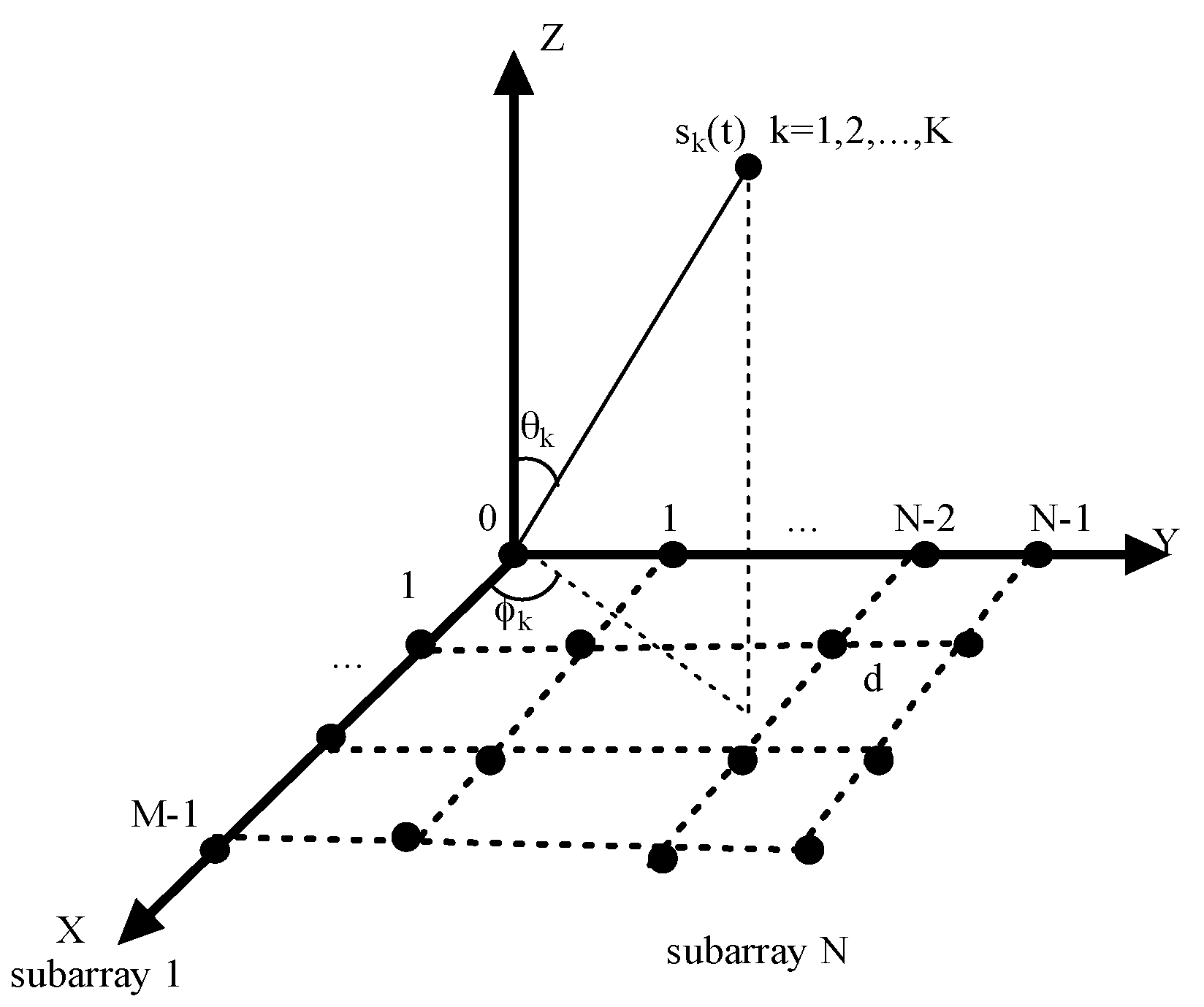
2. Data Model
3. Real-Valued PM Algorithm for 2D-DOA Estimation
3.1. Euler Transformation
3.2. 2D-DOA Estimation
- (1)
- Construct the matrix from Equation (5), and compute the covariance matrix of through Equation (8).
- (2)
- Estimation of the propagator from Equation (9), and then construct the matrix .
- (3)
- Construct the matrix and and perform the eigenvalue decomposition of .
- (4)
- Similarly, construct the matrix and and perform the eigenvalue decomposition of .
- (5)
- Finally, estimate the 2D-DOA through Equations (17) and (18).
4. Cramer-Rao Bounds and Analysis
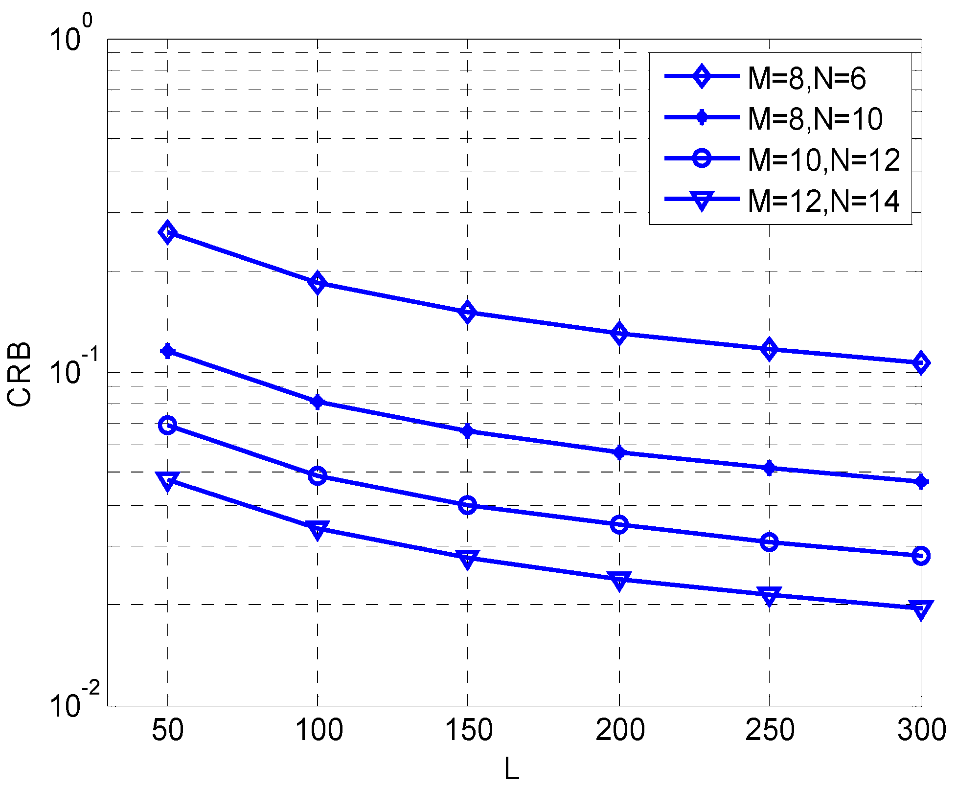
4.1. CRB
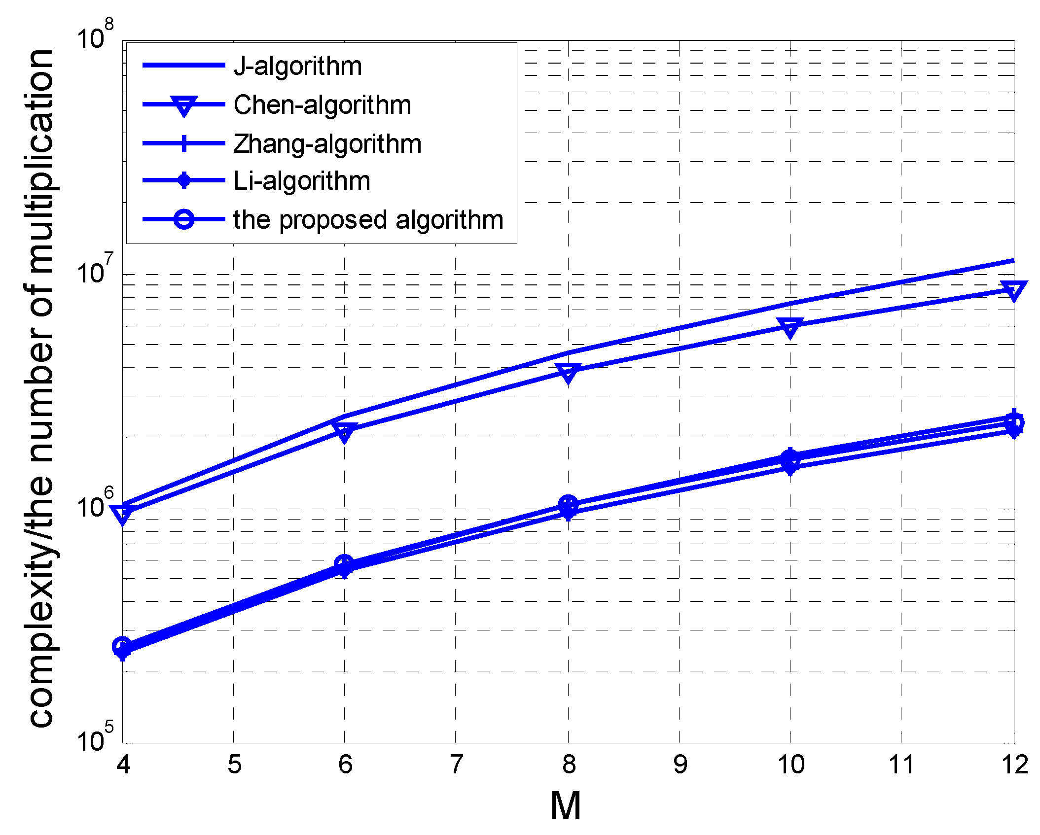
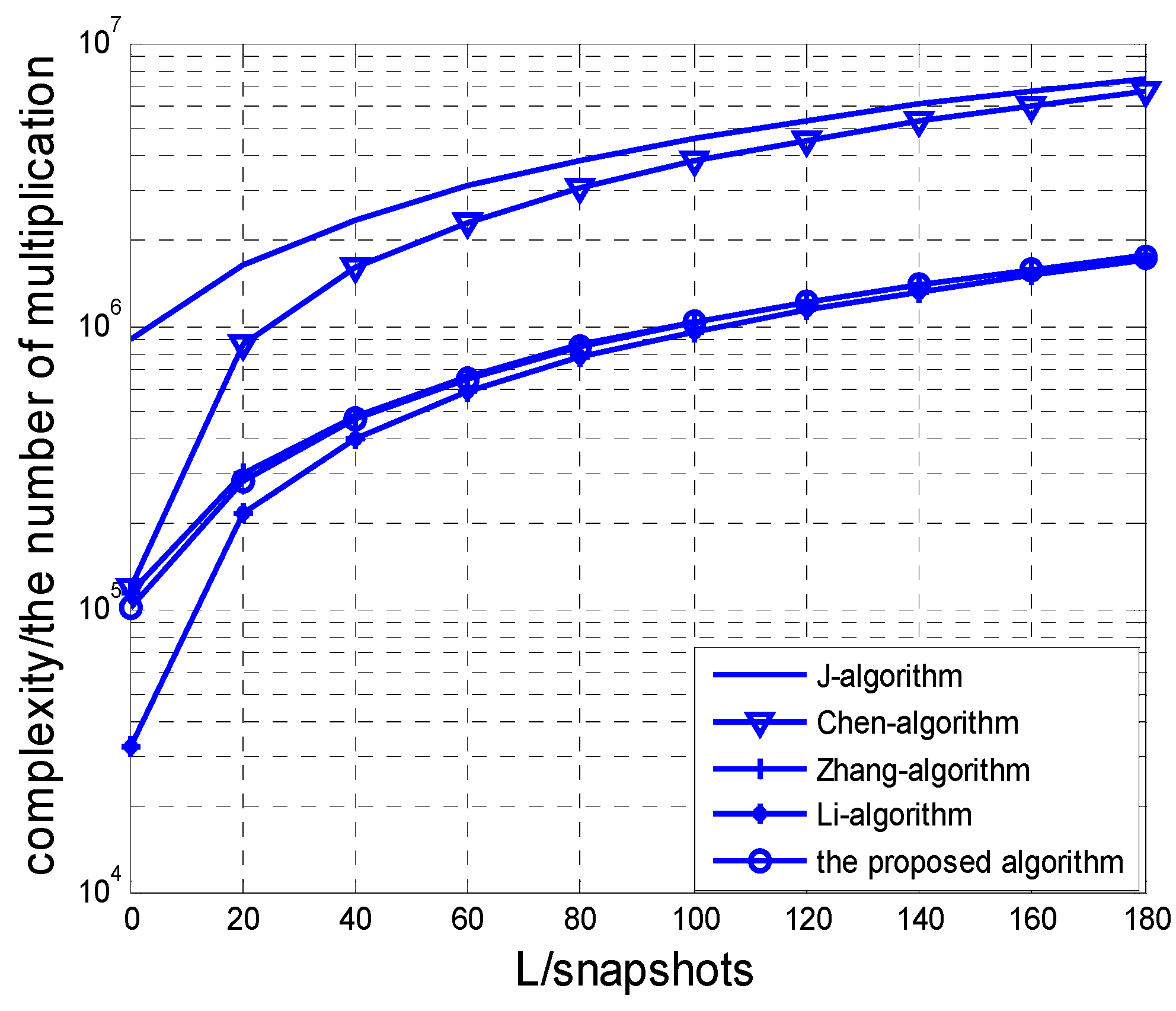
4.2. Complexity Analysis
- (1)
- The proposed algorithm has much lower computational load than the NC-PM and NC-ESPRIT algorithms because the proposed algorithm uses Euler transformation to convert complex arithmetic of noncircular PM to real arithmetic.
- (2)
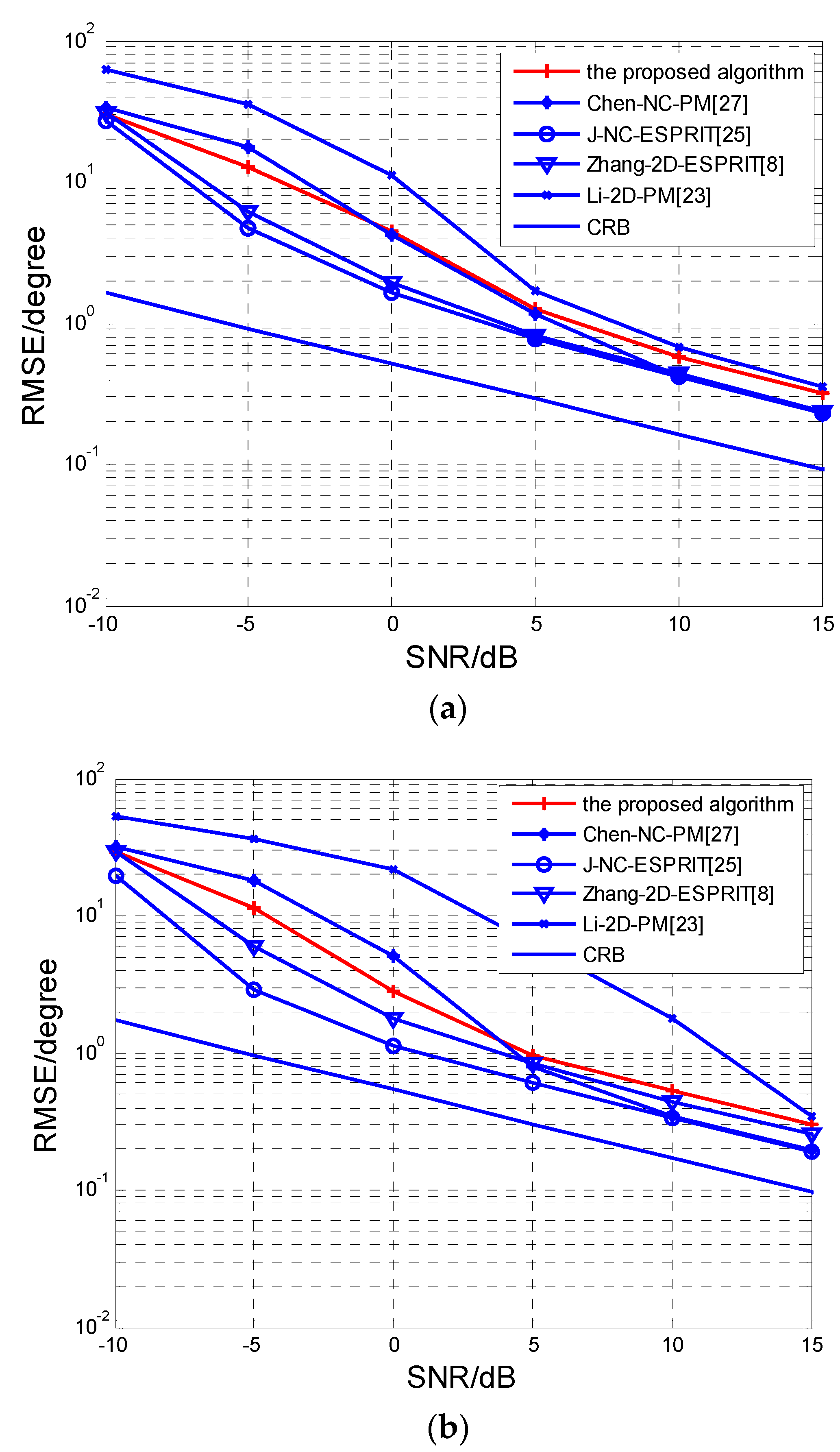
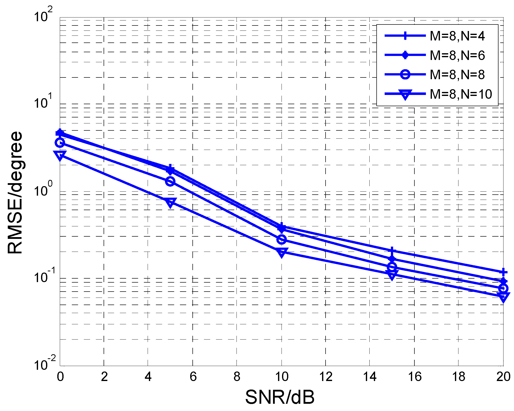
- The proposed algorithm has better estimation performance than the 2D-PM algorithm because the array aperture is doubled according to Equation (5).
- (3)
- The maximum number of discerned sources of our algorithm is dependent on Equation (5) and the real-valued PM method. Obviously, the maximum number of the identified sources of our proposed algorithm is , while 2D-PM is .
- (4)
- The proposed algorithm requires no extra matching calculation. The estimated 2D-DOA can automatically be matched.
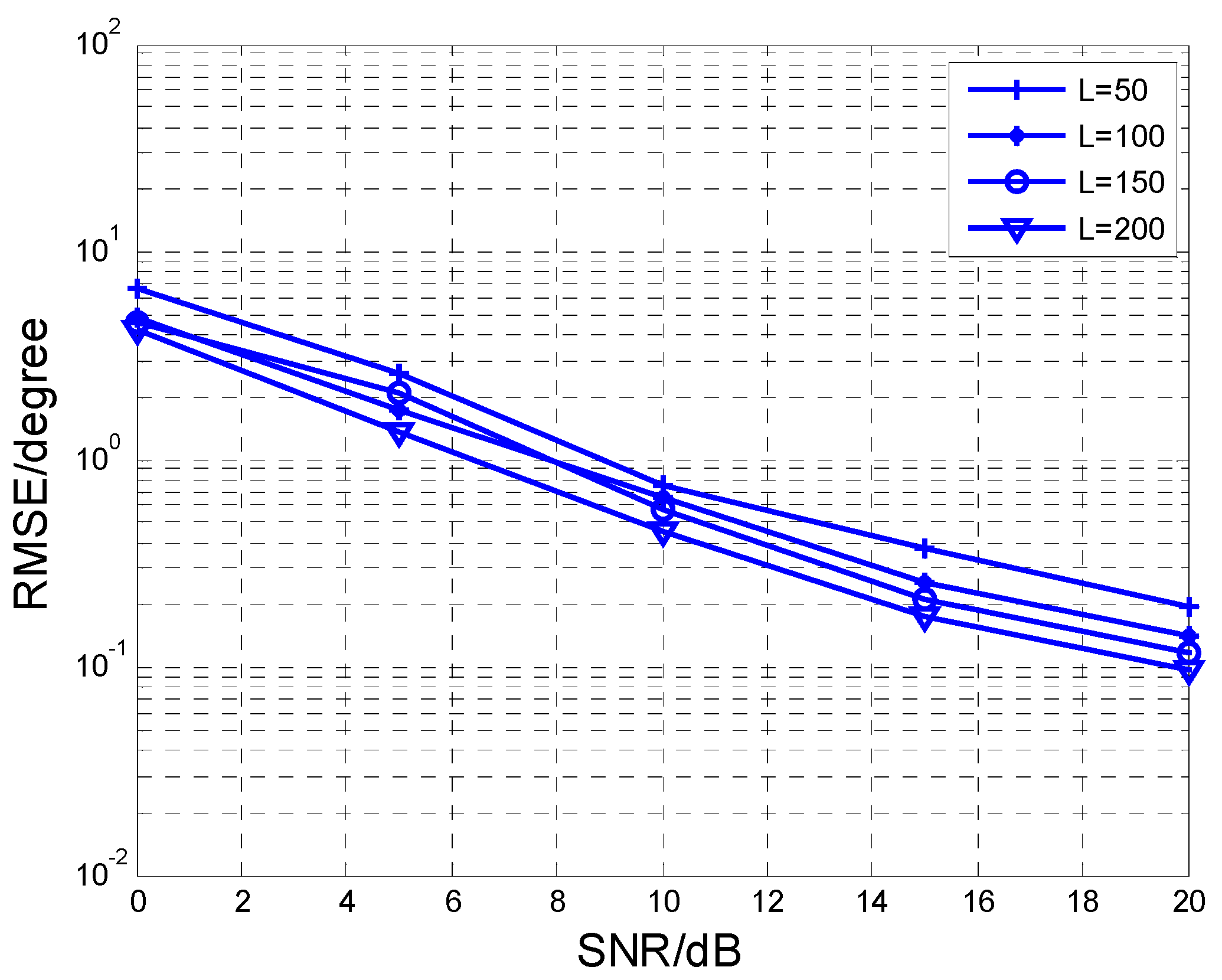
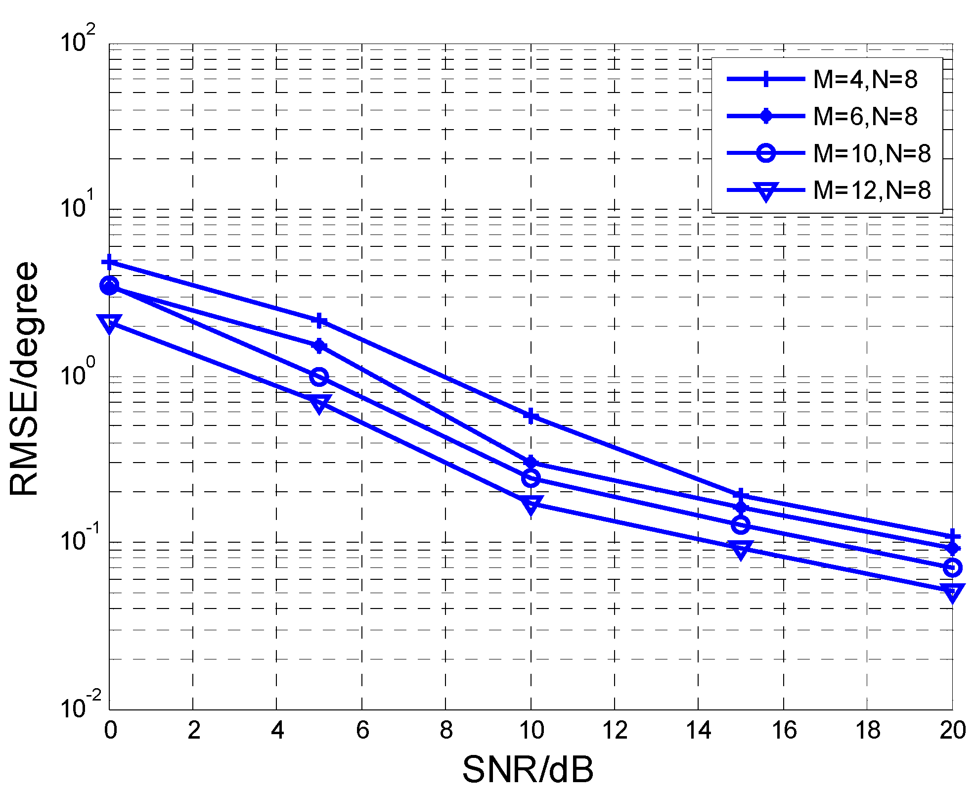
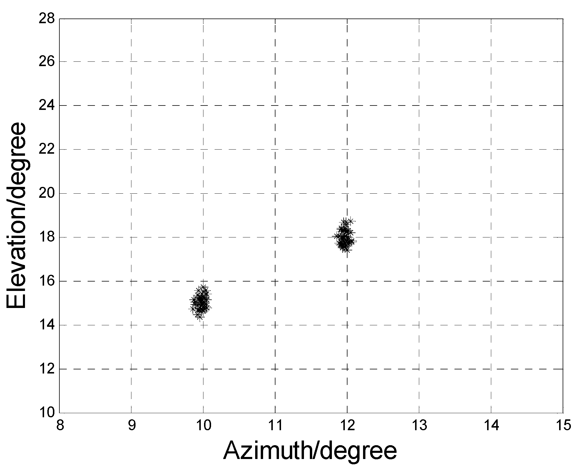
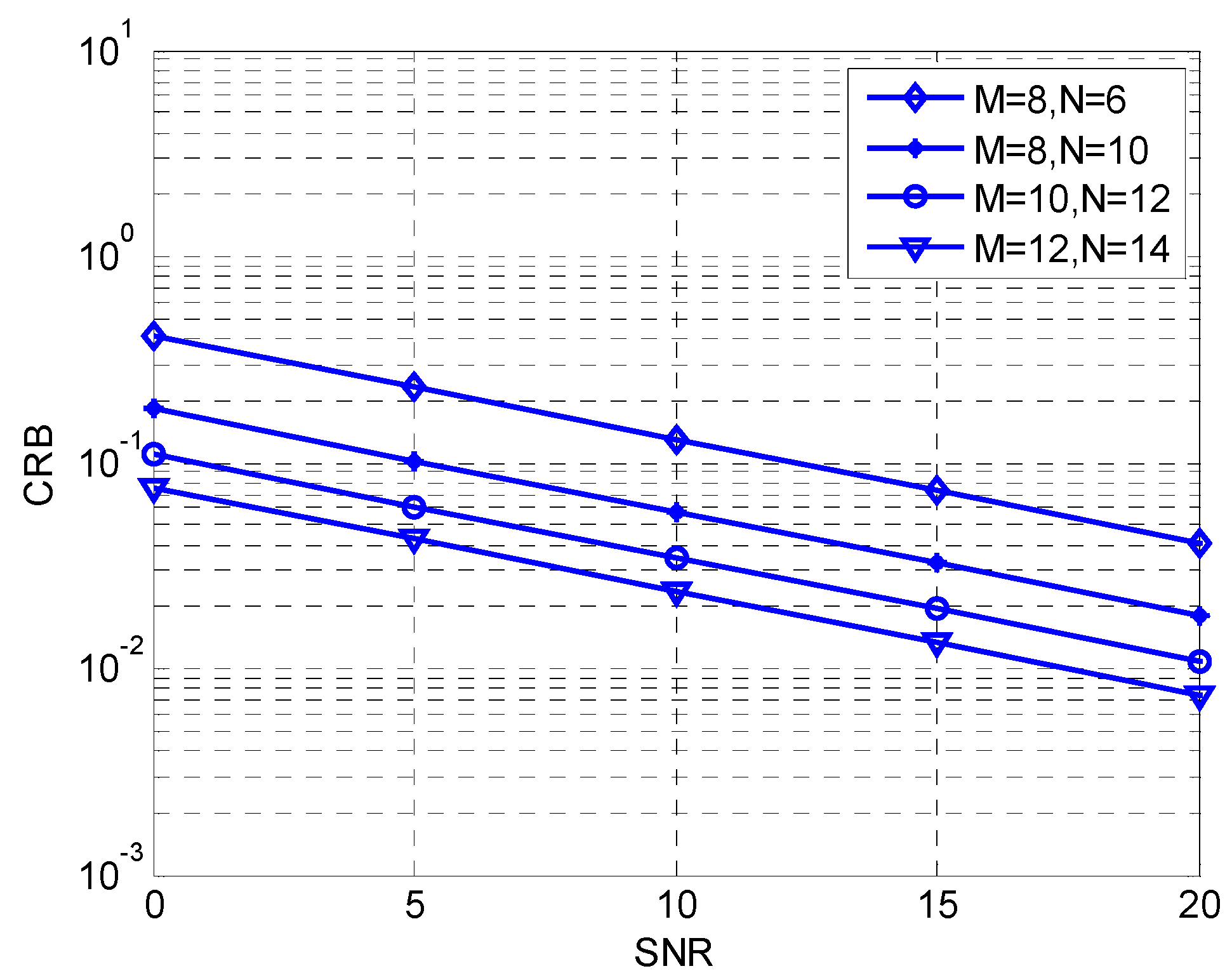
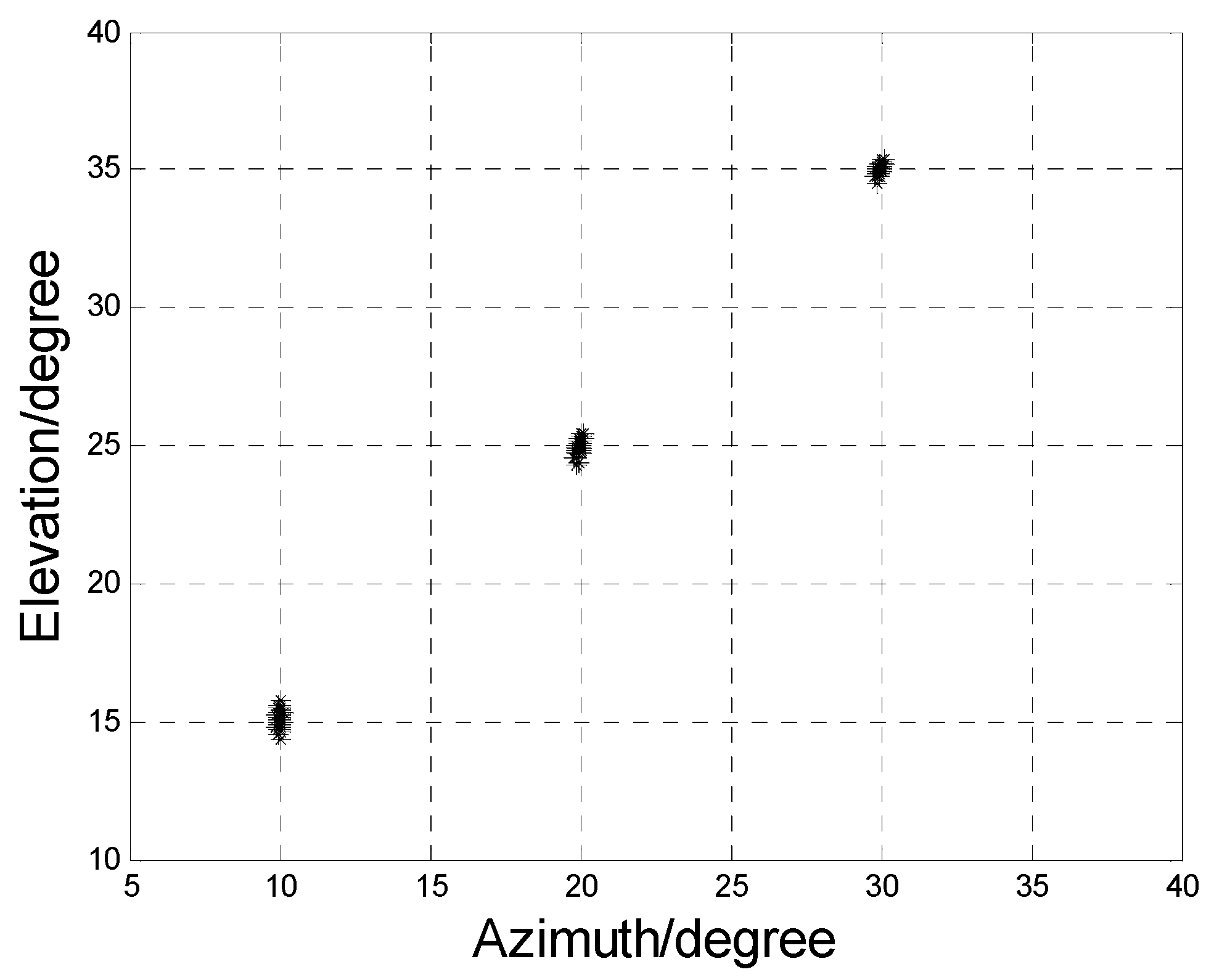
5. Simulation Results
6. Conclusions
Acknowledgments
Author Contributions
Conflicts of Interest
Abbreviations
| 2D-DOA | Two-dimensional direction of arrival |
| URA | Uniform rectangular planar array |
| PM | Propagator method |
| CRB | Crame–Rao bound |
| RMS | Real-valued multiplications |
| RMSE | Root mean square error |
| SNR | Signal-to-noise ratio |
References
- Min, S.; Seo, D.; Lee, K.B.; Kwon, H.M.; Lee, Y.H. Direction-of-arrival tracking scheme for DS/CDMA systems: Direction lock loop. IEEE Trans. Wirel. Commun. 2004, 3, 191–202. [Google Scholar] [CrossRef]
- Chiang, C.T.; Chang, A.C. DOA estimation in the asynchronous DS-CDMA system. IEEE Antennas Propag. 2003, 51, 40–47. [Google Scholar] [CrossRef]
- Yang, S.; Li, Y.; Zhang, K.; Tang, W. Multiple-parameter estimation method based on spatio-temporal 2-D processing for bistatic MIMO radar. Sensors 2015, 15, 31442–31452. [Google Scholar] [CrossRef] [PubMed]
- Zhang, X.F.; Zhou, M.; Li, J.F. A PARALIND decomposition-based coherent two-dimensional direction of arrival estimation algorithm for acoustic vector-sensor arrays. Sensors 2013, 13, 5302–5316. [Google Scholar] [CrossRef] [PubMed]
- Liang, H.; Cui, C.; Dai, L.; Yu, J. Reduced-dimensional DOA estimation based on ESPRIT algorithm in MIMO radar with L-shaped array. J. Electron. Inf. Technol. 2015, 37, 1828–1835. [Google Scholar]
- Wax, M.; Shan, T.J.; Kailath, T. Spatio-temporal spectral analysis by eigenstructure methods. IEEE Trans. Acoust. Speech Signal Process. 1984, 32, 817–827. [Google Scholar] [CrossRef]
- Zoltowski, M.D.; Haardt, M.; Mathews, C.P. Closed-form 2-D angle estimation with rectangular arrays in element space or beamspace via unitary ESPRIT. IEEE Trans. Signal Process. 1996, 44, 316–328. [Google Scholar] [CrossRef]
- Zhang, X.; Gao, X.; Chen, W. Improved blind 2D-direction of arrival estimation with L-shaped array using shift invariance property. J. Electromagn. Waves Appl. 2009, 23, 593–606. [Google Scholar] [CrossRef]
- Del Rio, J.E.F.; Catedra-Perez, M.F. The matrix pencil method for two-dimensional direction of arrival estimation employing an L-shaped array. IEEE Trans. Antennas Propag. 1997, 45, 1693–1694. [Google Scholar] [CrossRef]
- Clark, M.P.; Scharf, L.L. Two-dimensional modal analysis based on maximum likelihood. IEEE Trans. Signal Process. 1994, 42, 1443–1452. [Google Scholar] [CrossRef]
- Fang, W.H.; Lee, Y.C.; Chen, Y.T. Maximum likelihood 2-D DOA estimation via signal separation and importance sampling. IEEE Antennas Wirel. Propag. Lett. 2016, 16, 746–749. [Google Scholar] [CrossRef]
- Zhang, X.F.; Li, J.F.; Xu, L.Y. Novel two-dimensional DOA estimation with L-shaped array. EURASIP J. Adv. Signal Process. 2011, 50, 1–7. [Google Scholar] [CrossRef]
- Nie, X.; Li, L.P. A computationally efficient subspace algorithm for 2-D DOA estimation with L-shaped array. IEEE Signal Process. Lett. 2014, 21, 971–974. [Google Scholar]
- Wang, G.M.; Xin, J.M.; Zheng, N.N.; Sano, A. Computationally efficient subspace-based method for two-dimensional direction estimation with L-shaped array. IEEE Trans. Signal Process. 2011, 59, 3197–3212. [Google Scholar] [CrossRef]
- Wei, Y.S.; Guo, X.J. Pair-matching method by signal covariance matrices for 2D-DOA estimation. IEEE Antennas Wirel. Propag. Lett. 2014, 13, 1199–1202. [Google Scholar]
- Zhang, W.; Liu, W.; Wang, J.; Wu, S.L. Computationally efficient 2D DOA estimation for unform rectangular arrays. Multidimens. Syst. Signal Process. 2014, 25, 847–857. [Google Scholar] [CrossRef]
- Yu, H.X.; Qiu, X.F.; Zhang, X.F. Two-dimensional direction of arrival estimation for rectangular array via compressive sensing trilinear model. Int. J. Antenna Propag. 2015, 2015, 297572. [Google Scholar] [CrossRef]
- Xu, X.; Ye, Z. Two-dimensional direction of arrival estimation by exploiting the symmetric configuration of uniform rectangular array. IET Radar Sonarav. Navig. 2012, 6, 307–313. [Google Scholar] [CrossRef]
- Wu, H.; Hou, C.P.; Chen, H.; Liu, W.; Wang, Q. Direction finding and mutual coupling estimation for uniform rectangular arrays. Signal Process. 2015, 117, 61–68. [Google Scholar] [CrossRef]
- Gu, J.F.; Zhu, W.P.; Swamy, M.N.S. Joint 2D DOA estimation via sparse L-shaped array. IEEE Trans. Signal Process. 2015, 63, 1171–1182. [Google Scholar] [CrossRef]
- Marcos, S.; Marsal, A.; Benider, M. The propagator method for sources bearing estimation. Signal Process. 1995, 42, 121–138. [Google Scholar] [CrossRef]
- Wu, Y.; Liao, G.S.; So, H.C. A fast algorithm for 2-D direction of-arrival estimation. Signal Process. 2003, 83, 1827–1831. [Google Scholar] [CrossRef]
- Li, J.F.; Zhang, X.F.; Chen, H. Improved two-dimensional DOA estimation algorithm for two-parallel uniform linear arrays using propagator method. Signal Process. 2012, 92, 3032–3038. [Google Scholar] [CrossRef]
- Abeida, H.; Delmas, J.P. MUSIC-like estimation of direction of arrival for noncircular sources. IEEE Trans. Signal Process. 2006, 54, 2678–2690. [Google Scholar] [CrossRef]
- Steinwandt, J.; Roemer, F.; Haardt, M. Performance analysis of ESPRIT-type algorithms for non-circular sources. In Proceedings of the 38th IEEE International Conference on Acoustics, Speech, and Signal Processing (ICASSP 13), Vancouver, BC, Canada, 26–31 May 2013; pp. 3986–3990. [Google Scholar]
- Zhang, L.; Lv, W.H.; Zhang, X.F. 2D-DOA estimation of noncircular signals for uniform rectangular array via NC-PARAFAC method. Int. J. Electron. 2016, 103, 1839–1856. [Google Scholar] [CrossRef]
- Chen, C.Q.; Wang, C.H.; Zhang, X.F. DOA and Noncircular phase estimation of noncircular signal via an improved noncircular rotational invariance propagator method. Math. Probl. Eng. 2015, 2015, 235173. [Google Scholar] [CrossRef]
- Picinbono, B. On circularity. IEEE Trans. Signal Process. 1994, 42, 3473–3482. [Google Scholar] [CrossRef]
- Stoica, P.; Nehorai, A. Performance study of conditional and unconditional direction-of-arrival estimation. IEEE Trans. Acoust. Speech Signal Process. 1990, 38, 1783–1795. [Google Scholar] [CrossRef]


© 2017 by the authors. Licensee MDPI, Basel, Switzerland. This article is an open access article distributed under the terms and conditions of the Creative Commons Attribution (CC BY) license (http://creativecommons.org/licenses/by/4.0/).
Share and Cite
Xu, L.; Wen, F. Fast Noncircular 2D-DOA Estimation for Rectangular Planar Array. Sensors 2017, 17, 840. https://doi.org/10.3390/s17040840
Xu L, Wen F. Fast Noncircular 2D-DOA Estimation for Rectangular Planar Array. Sensors. 2017; 17(4):840. https://doi.org/10.3390/s17040840
Chicago/Turabian StyleXu, Lingyun, and Fangqing Wen. 2017. "Fast Noncircular 2D-DOA Estimation for Rectangular Planar Array" Sensors 17, no. 4: 840. https://doi.org/10.3390/s17040840
APA StyleXu, L., & Wen, F. (2017). Fast Noncircular 2D-DOA Estimation for Rectangular Planar Array. Sensors, 17(4), 840. https://doi.org/10.3390/s17040840