Accurate Determination of the Frequency Response Function of Submerged and Confined Structures by Using PZT-Patches†

 , and
, and
Abstract
:1. Introduction
2. Modal Analysis Model
2.1. Generic Equations for Modal Analysis
- Natural frequency: is the natural frequency of the corresponding mode r.
- Damping: is the damping factor and determines the amplitude of the structural response when the system is close to a resonance condition .
- Mode shapes: define the deformation shape that dominates the structure close to resonance condition .
- Scaling Factor: is a constant factor defined for each mode r and has an influence on the amplitude of the response.
2.2. Comments for Fluid-Structure Interaction Problems
2.3. Generic Equations for a PZT-Actuator
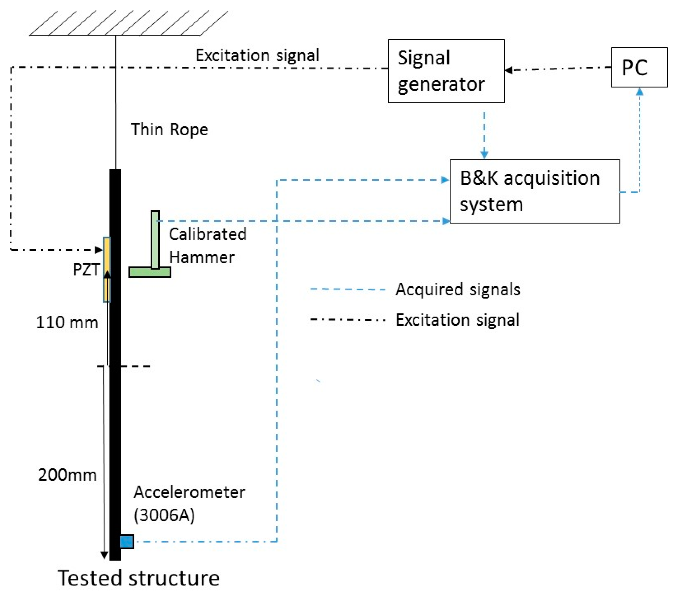
3. Experimental Set-Up and Signal Analysis
3.1. Equipement Used
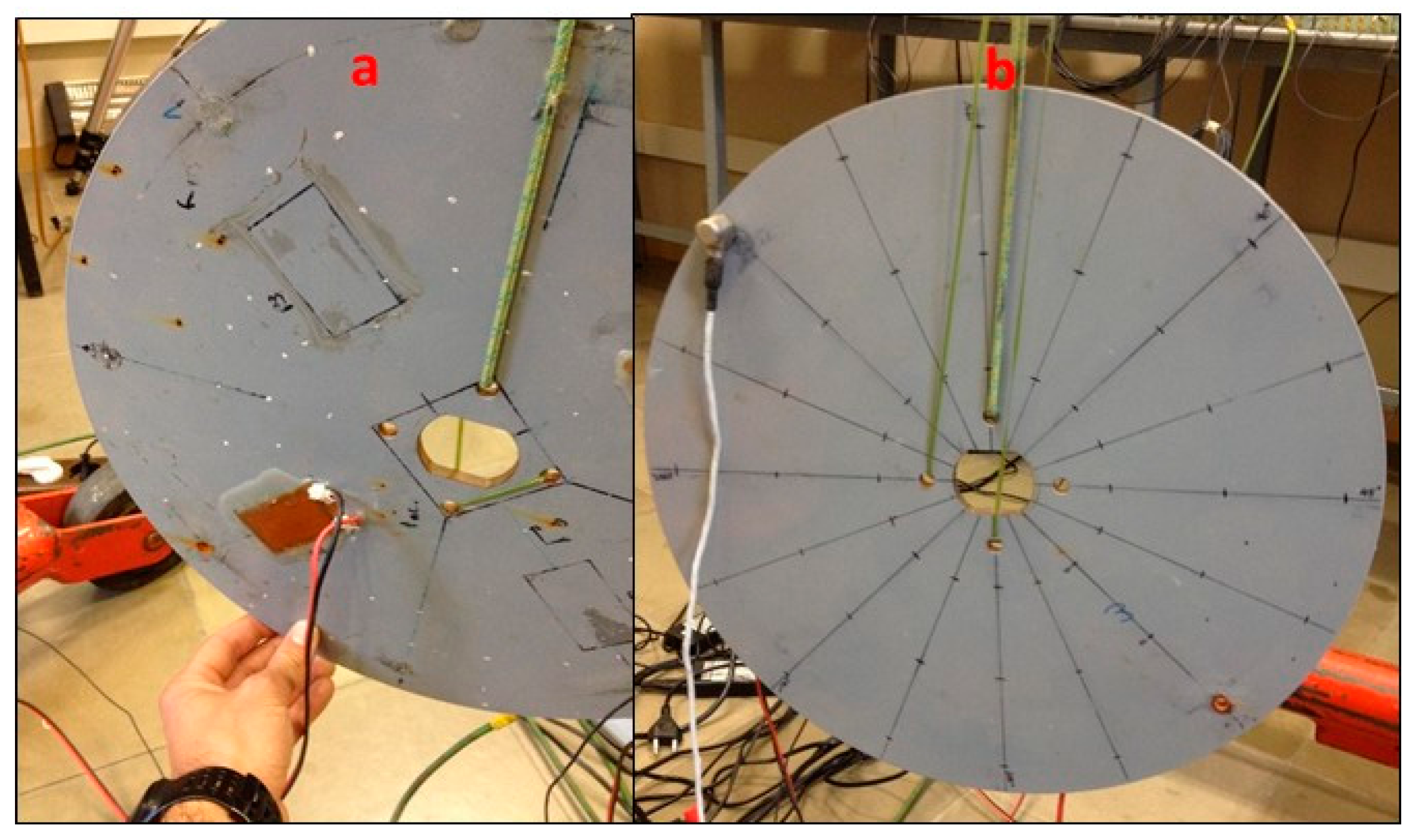
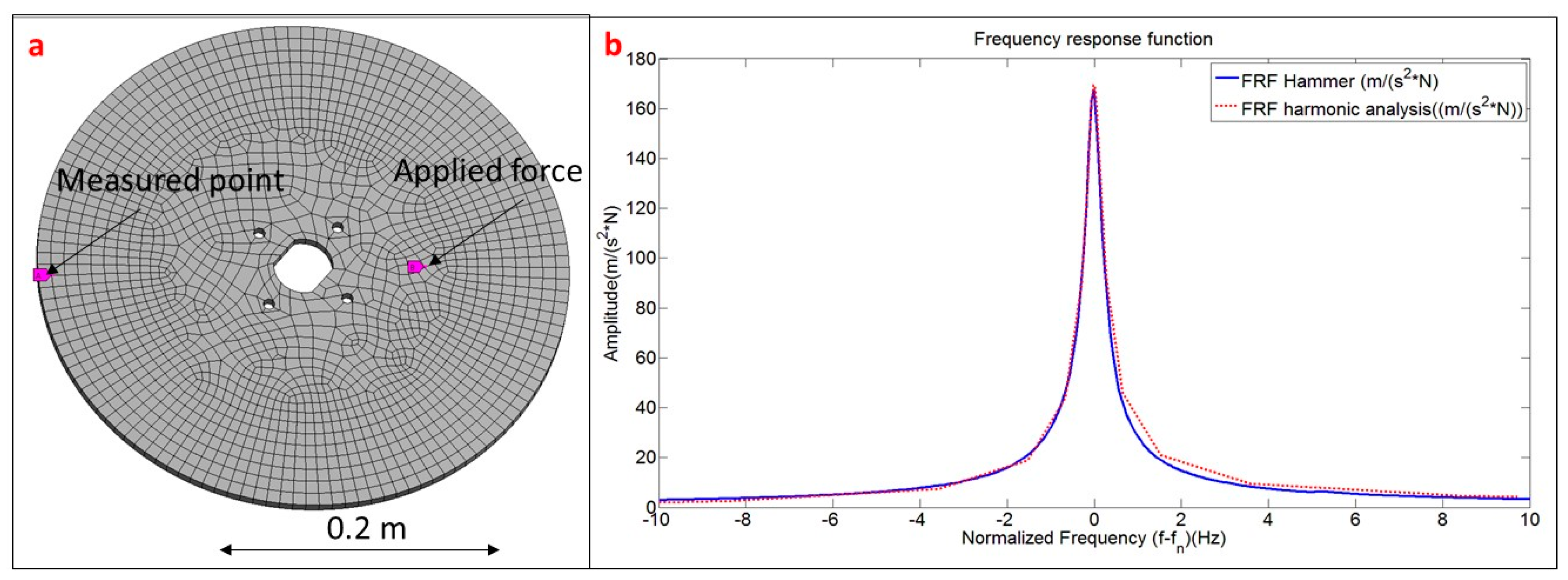
3.1.1. Tested Structure
3.1.2. PZT-Patch
3.1.3. Accelerometer
3.1.4. Instrumented Hammer
3.1.5. Signal Generator and Amplifier
3.1.6. Acquisition System
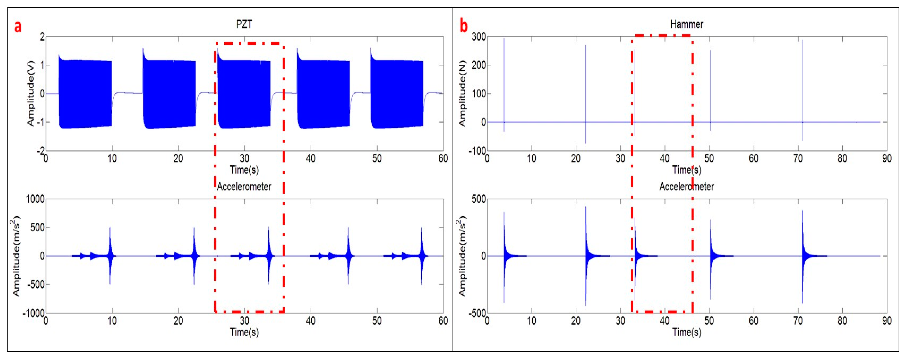
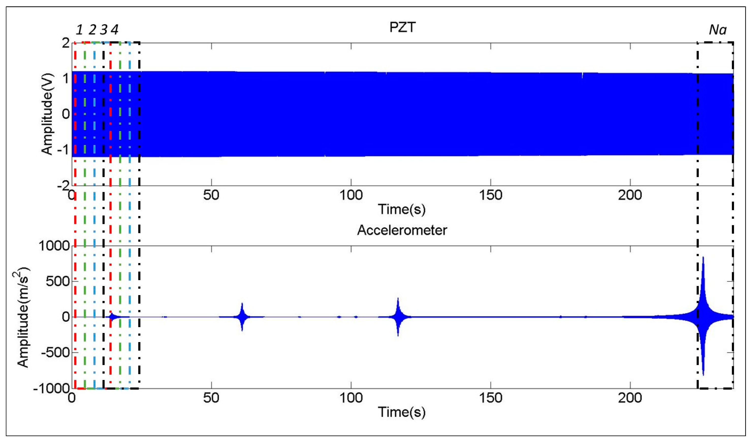
3.2. Excitation Characteristic and Signal Analysis
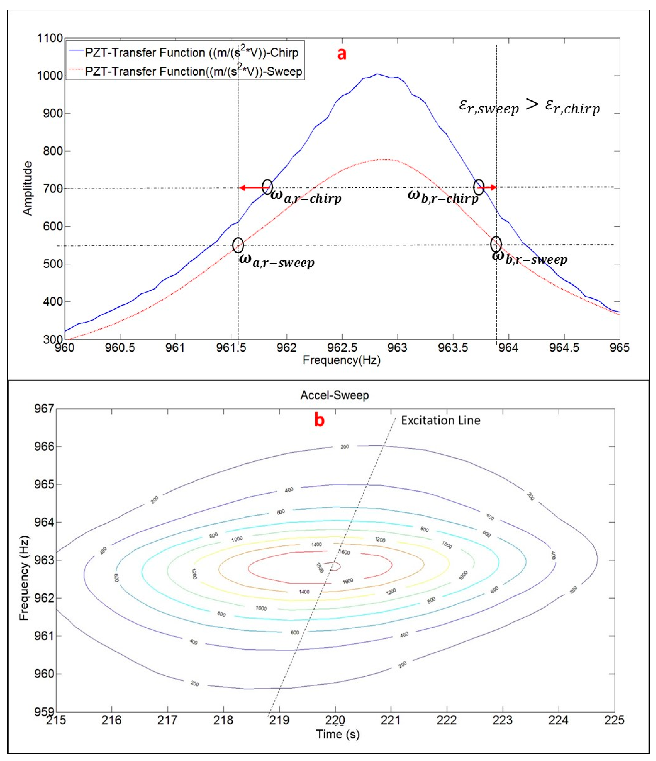
3.2.1. Chirp (PZT)
3.2.2. Sweep
3.2.3. Hammer
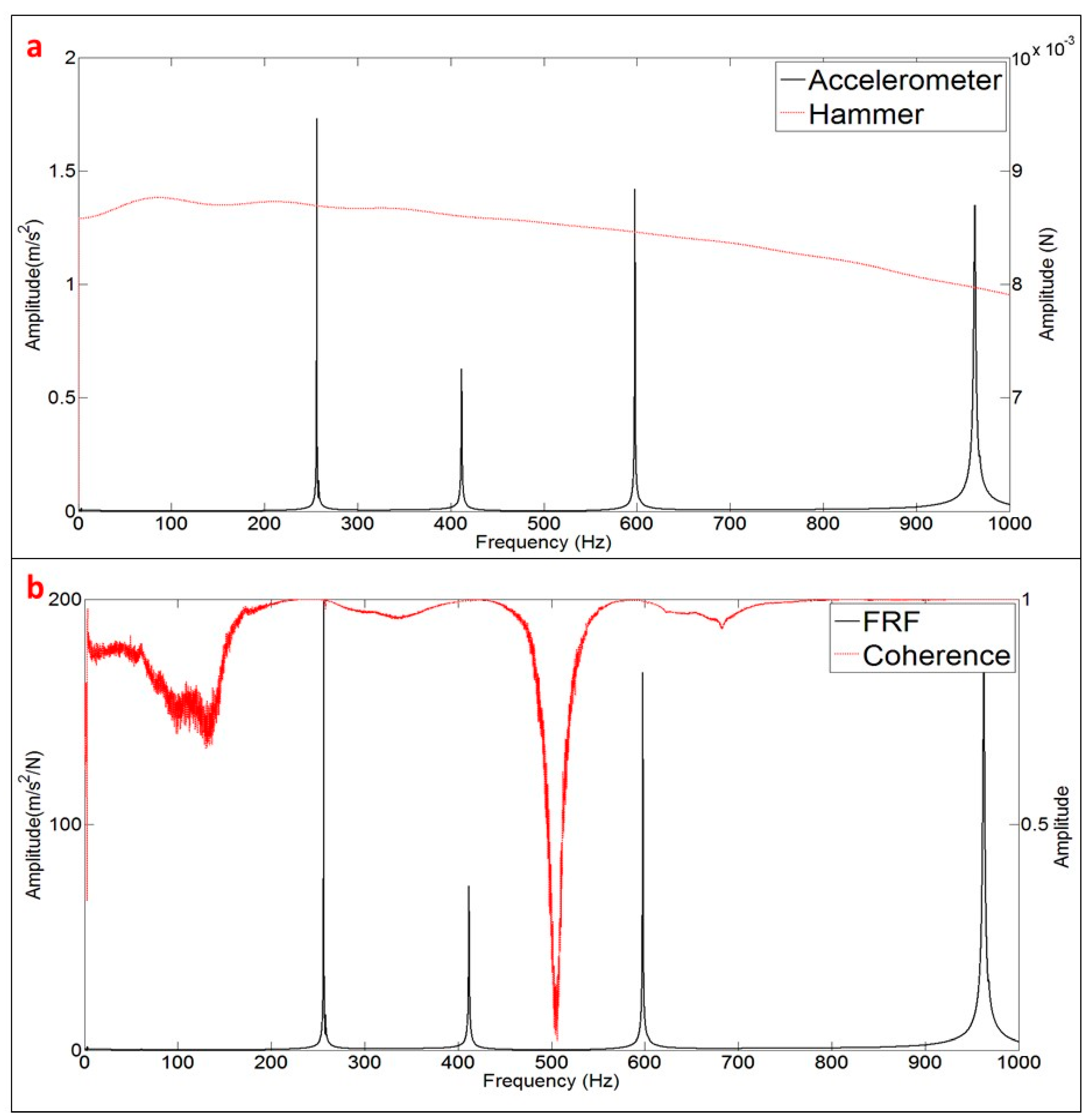
3.2.4. Signal Analysis
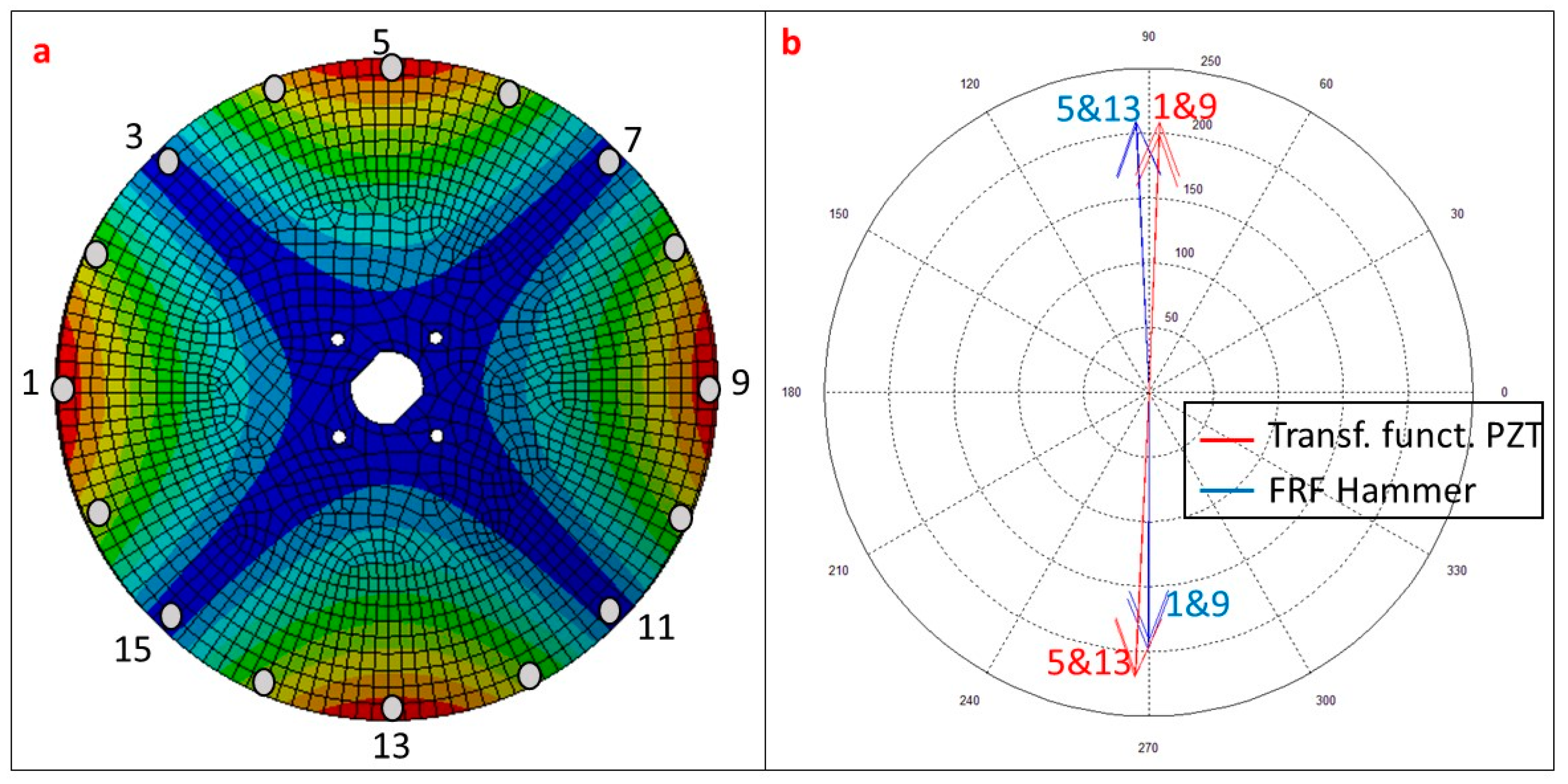
3.3. Tests Performed (Configurations)
3.3.1. Structure Suspended in Air
3.3.2. Structure Submerged in Water (Infinite Medium)
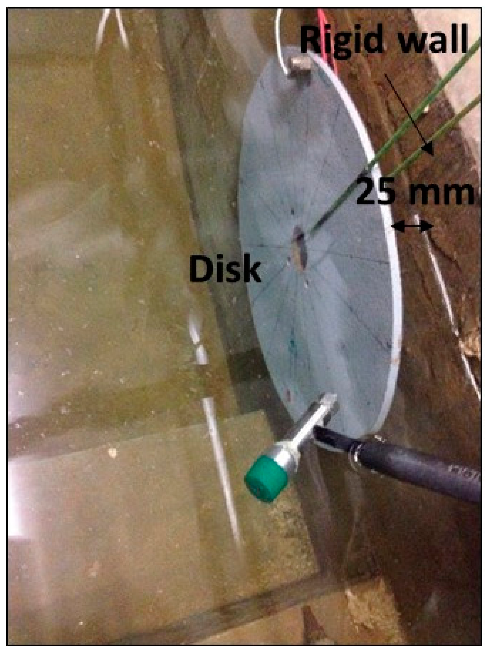
3.3.3. Structure Submerged in Water with a Nearby Rigid Wall
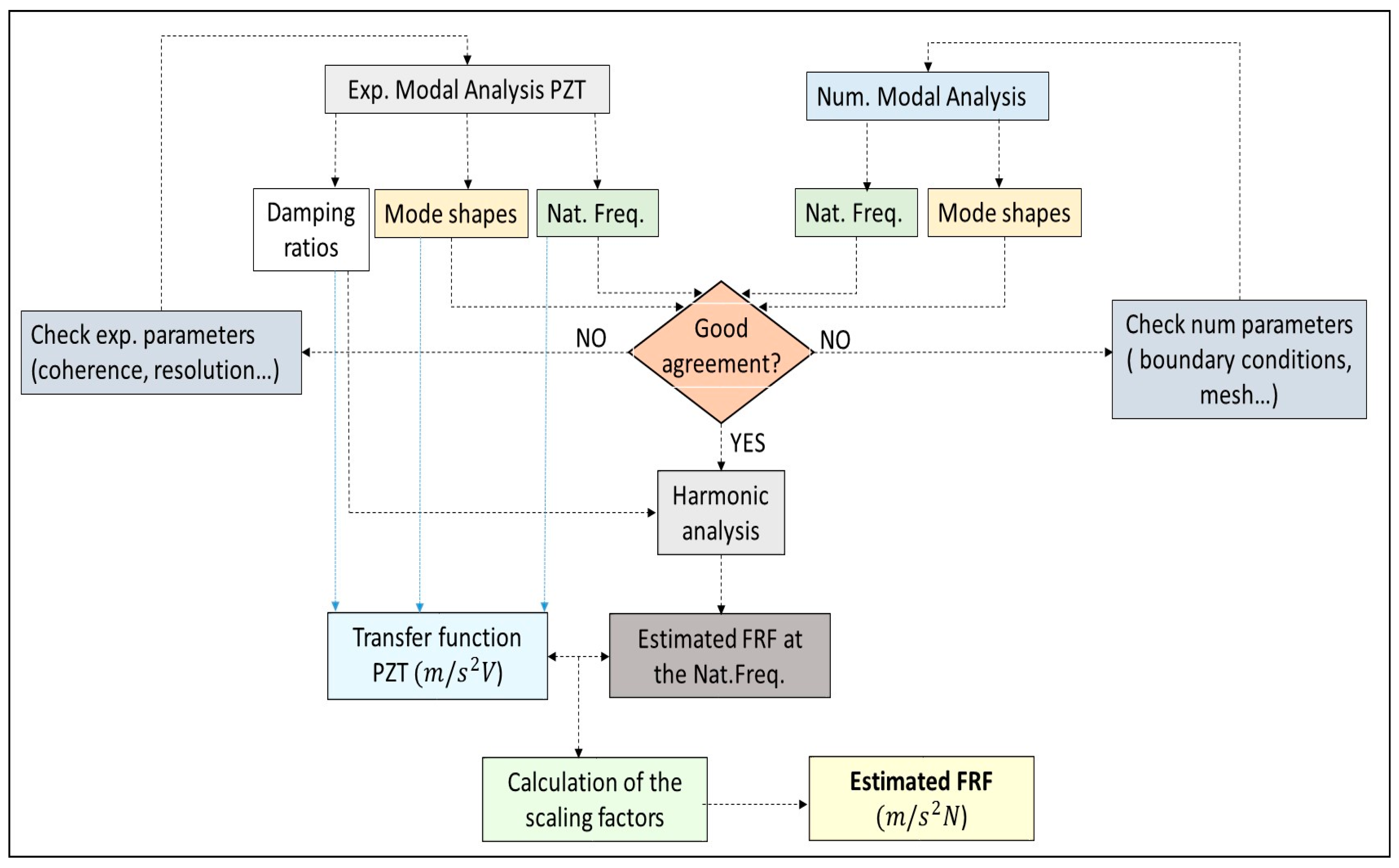
4. Methodology to Determine the FRF of a Structure by Means of PZT Excitation
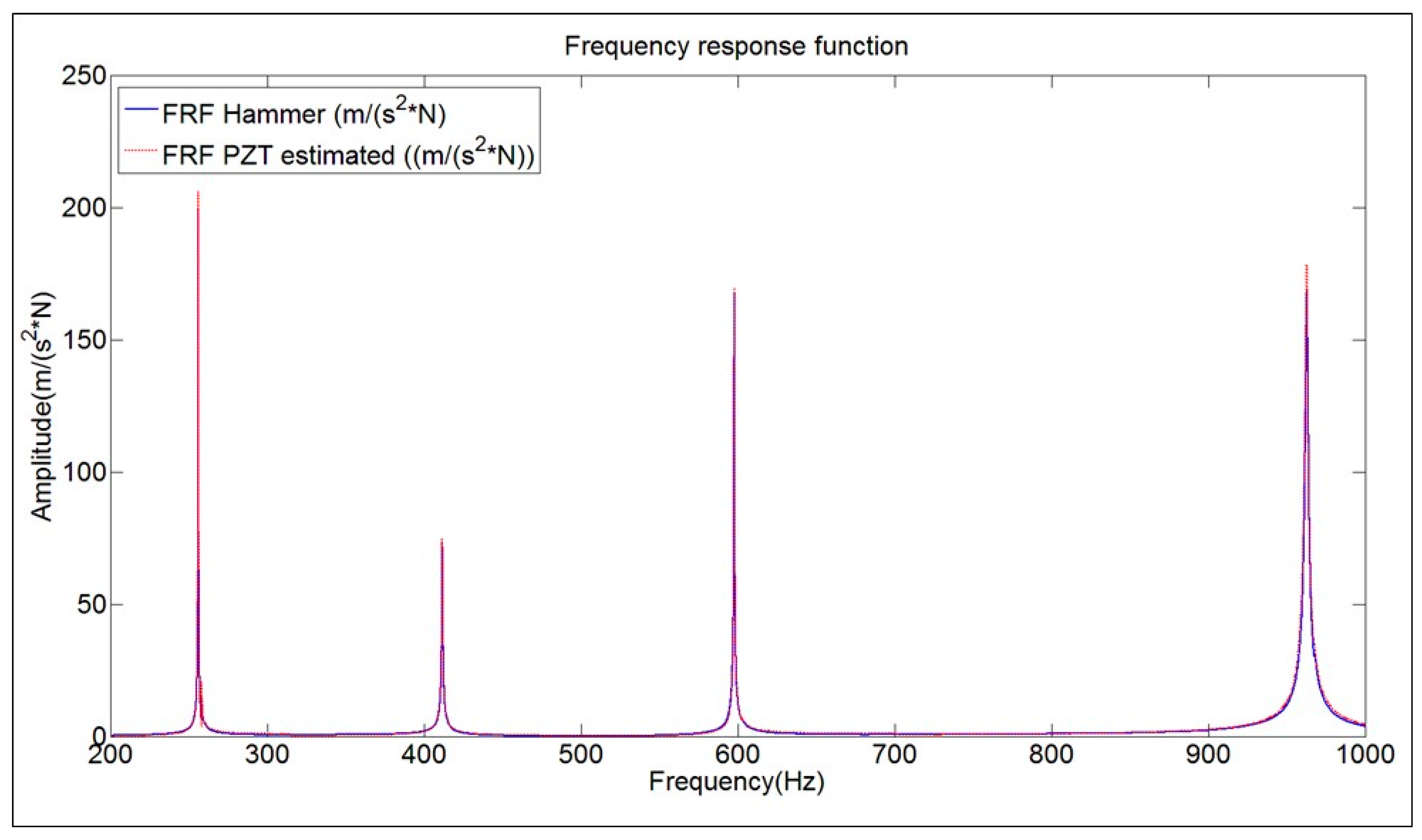
4.1. Natural Frequencies
4.2. Mode Shapes
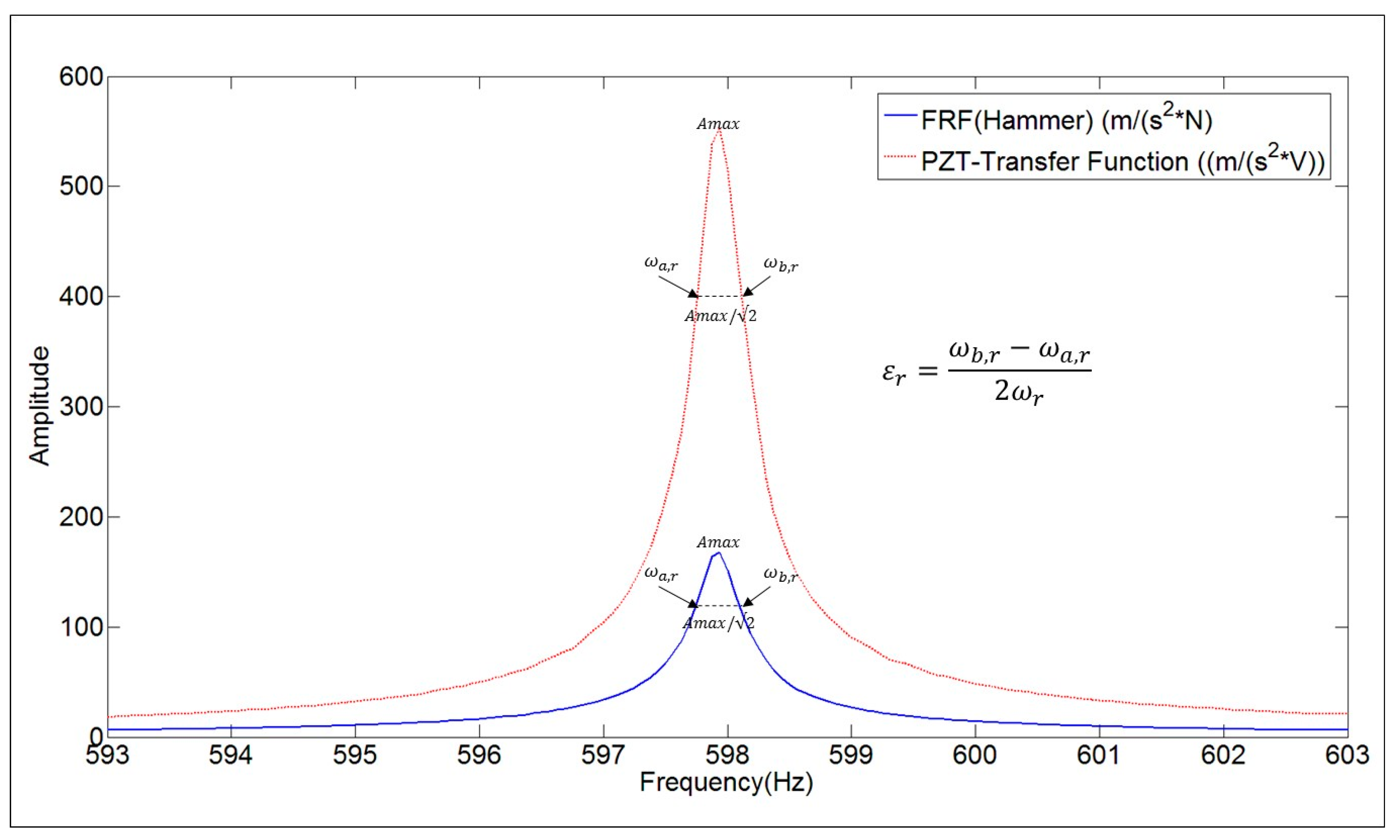
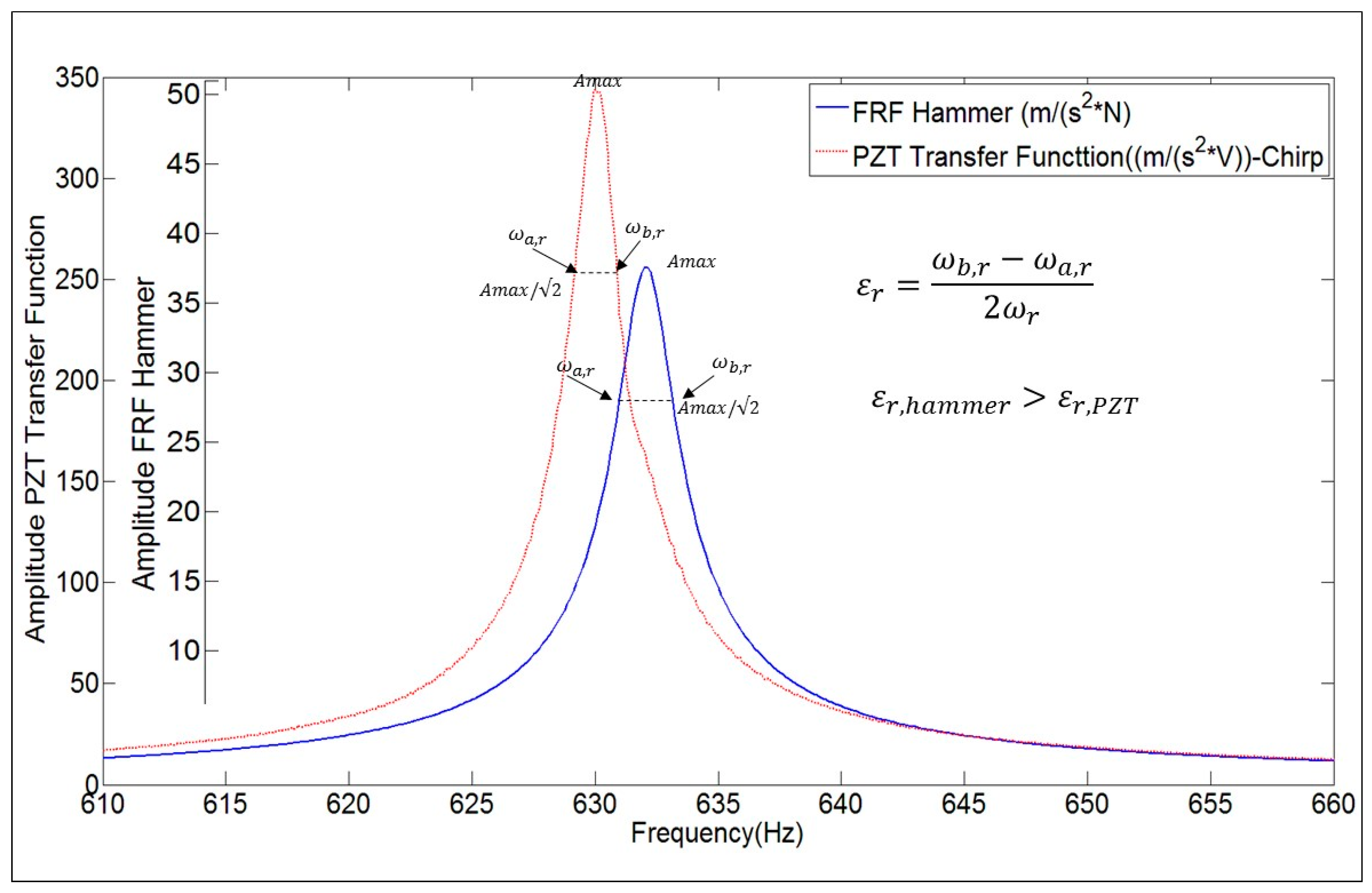
4.3. Damping Ratio
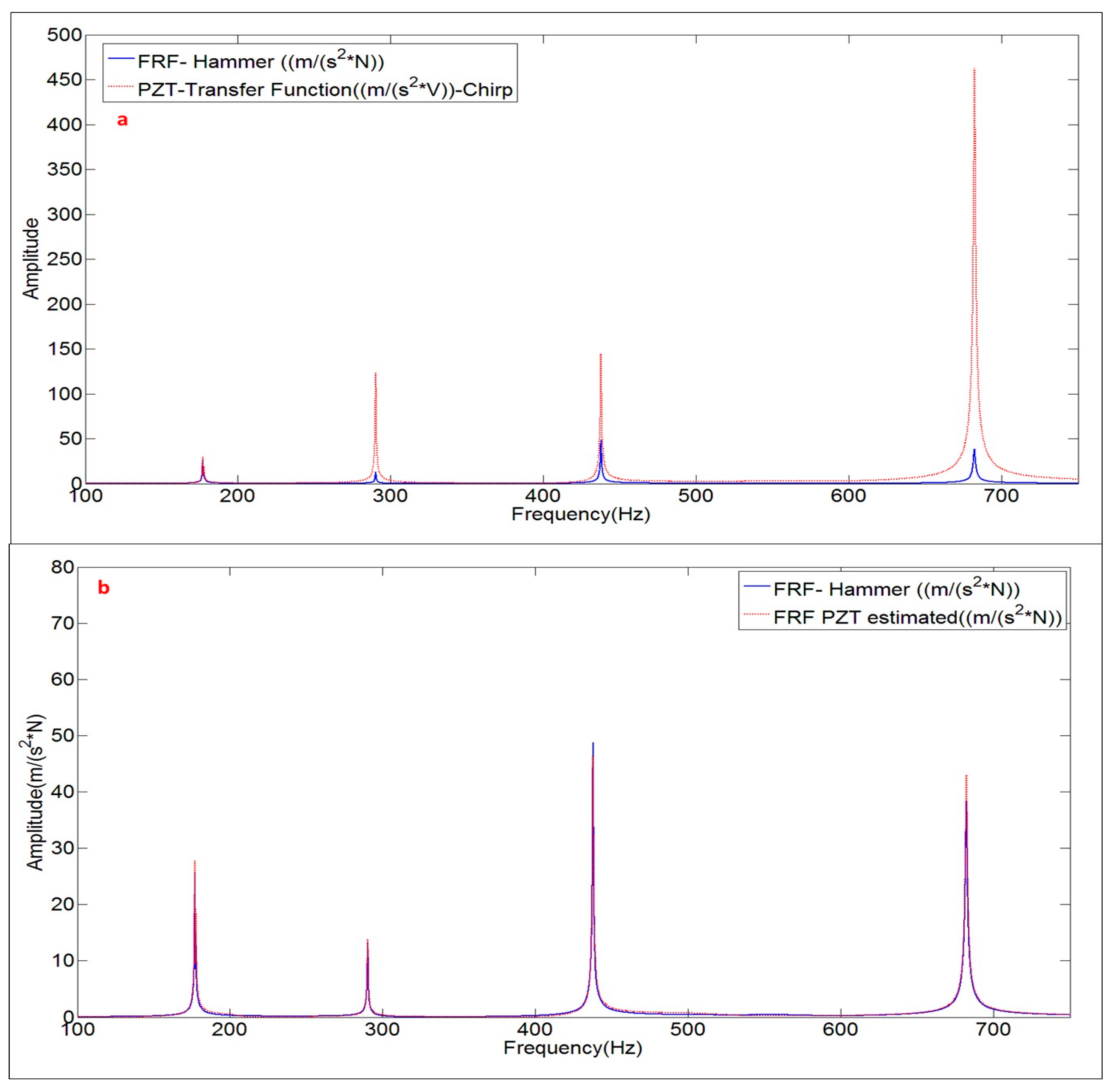
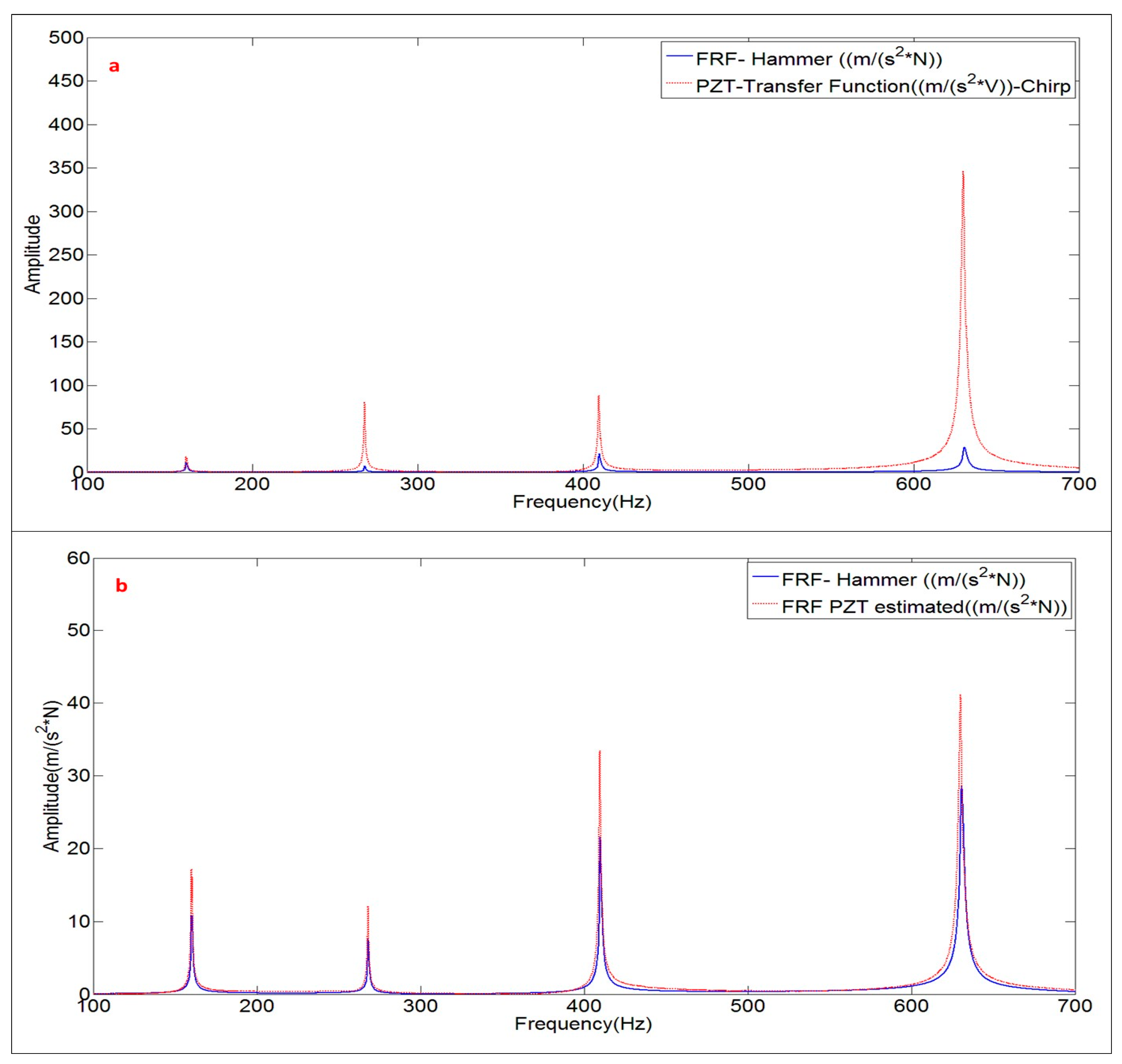
4.4. Proccedure to Estimate the Complete FRF
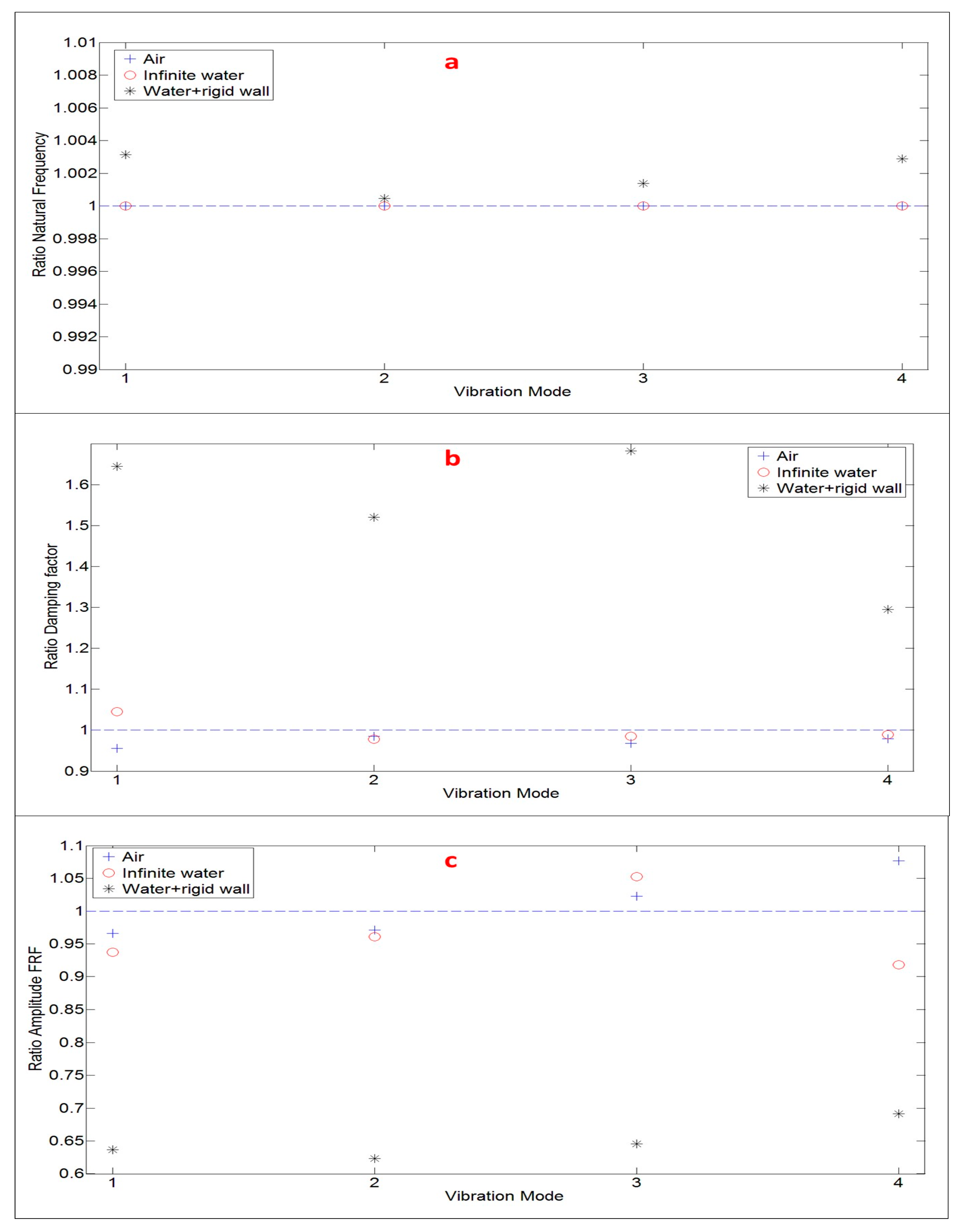
5. Determination of the FRF for Submerged Structures with Nearby Rigid Walls
5.1. FRF of the Structure with Infinite Water Medium
5.2. FRF of the Structure Close to a Rigid Wall
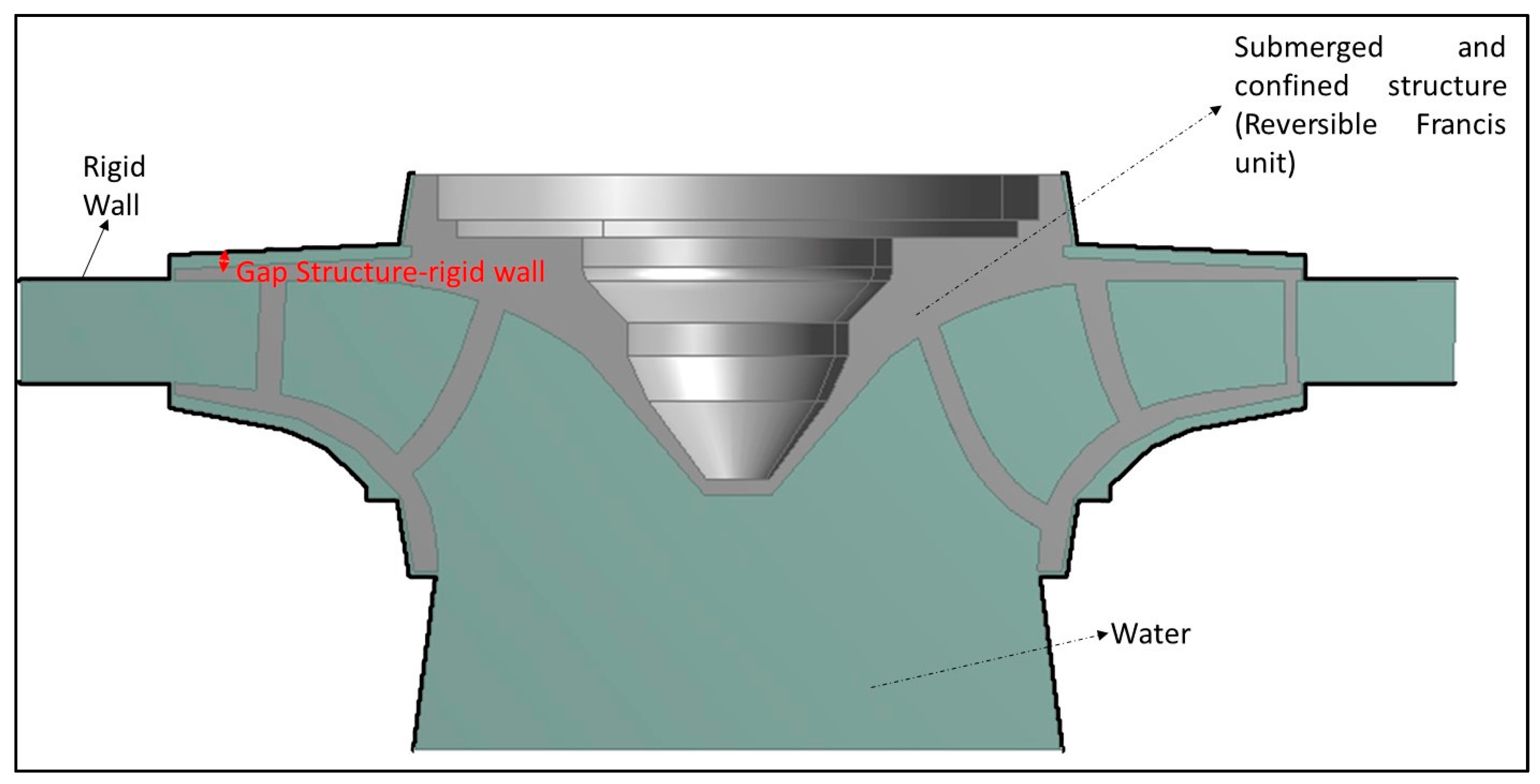
5.3. Potential Application in a Real Submerged and Confined Structure
6. Conclusions and Future Perspectives
Acknowledgments
Author Contributions
Conflicts of Interest
References
- Ewins, D.J. Modal Testing Theory and Practice; Research Studies Press: Letchworth, UK, 1984. [Google Scholar]
- Heylen, W. Modal Analysis Theory and Testing; Katholieke Universiteit Leuven: Leuven, Belgium, 2007. [Google Scholar]
- Hearn, G.; Testa, R.B. Modal analysis for damage detection in structures. J. Struct. Eng. 1991, 117, 3042–3063. [Google Scholar] [CrossRef]
- Hermans, L.; van der Auweraer, H. Modal testing and analysis of structures under operational conditions: Industrial applications. Mech. Syst. Signal Process. 1999, 13, 193–216. [Google Scholar] [CrossRef]
- Egusquiza, E.; Valero, C.; Huang, X.; Jou, E.; Guardo, A.; Rodriguez, C. Failure investigation of a large pump-turbine runner. Eng. Fail. Anal. 2012, 23, 27–34. [Google Scholar] [CrossRef]
- Ohashi, H. Case Study of Pump Failure Due to Rotor-Stator Interaction. Int. J. Rotat. Mach. 1994, 1, 53–60. [Google Scholar] [CrossRef]
- Bi, S.; Ren, J.; Wang, W.; Zong, G. Elimination of transducer mass loading effects in shaker modal testing. Mech. Syst. Signal Process. 2013, 38, 265–275. [Google Scholar] [CrossRef]
- Wang, X.; Huang, Z. Feedback Control and Optimization for Rotating Disk Flutter Suppression with Actuators Patches. AIAA J. 2006, 44, 892–900. [Google Scholar] [CrossRef]
- Yan, T.; Xu, X.; Han, J.; Lin, R.; Ju, B.; Li, Q. Optimization of Sensing and Feedback Control for Vibration/Flutter of Rotating Disk by PZT Actuators via Air Coupled Pressure. Sensors 2011, 11, 3094–3116. [Google Scholar] [CrossRef] [PubMed]
- Yang, Z.; Guo, S.; Yang, J.; Hu, Y. Electrically forced vibration of an elastic plate with a finite piezoelectric actuator. J. Sound Vib. 2009, 321, 242–253. [Google Scholar] [CrossRef]
- Sekouri, E.M.; Hu, Y.-R.; Ngo, A.D. Modeling of a circular plate with piezoelectric actuators. Mechatronics 2004, 14, 1007–1020. [Google Scholar] [CrossRef]
- Cheng, C.C.; Lin, C.C. An impedance approach for vibration response synthesis using multiple PZT actuators. Sens. Actuators A Phys. 2005, 118, 116–126. [Google Scholar] [CrossRef]
- Presas, A.; Egusquiza, E.; Valero, C.; Valentin, D.; Seidel, U. Feasibility of Using PZT Actuators to Study the Dynamic Behavior of a Rotating Disk due to Rotor-Stator Interaction. Sensors 2014, 14, 11919–11942. [Google Scholar] [CrossRef] [PubMed]
- Gomis-Bellmunt, O.; Ikhouanne, F.; Montesinos-Miracle, D. Control of a piezoelectric actuator considering hysteresis. J. Sound Vib. 2009, 326, 383–399. [Google Scholar] [CrossRef]
- Presas, A.; Valentin, D.; Egusquiza, E.; Valero, C.; Seidel, U. Influence of the rotation on the natural frequencies of a submerged-confined disk in water. J. Sound Vib. 2015, 337, 161–180. [Google Scholar] [CrossRef]
- Presas, A.; Valentin, D.; Egusquiza, E.; Valero, C.; Seidel, U. On the detection of natural frequencies and mode shapes of submerged rotating disk-like structures from the casing. Mech. Syst. Signal Process. 2015, 60, 547–570. [Google Scholar] [CrossRef]
- Presas, A.; Valero, C.; Huang, X.; Egusquiza, E.; Farhat, M.; Avellan, F. Analysis of the Dynamic Response of Pump-Turbine Runners-Part I: Experiment; IOP Conference Series: Earth and Environmental Science, 2012; IOP Publishing: Bristol, UK, 2012; p. 052015. [Google Scholar]
- De La Torre, O.; Escaler, X.; Egusquiza, E.; Farhat, M. Experimental investigation of added mass effects on a hydrofoil under cavitation conditions. J. Fluids Struct. 2013, 39, 173–187. [Google Scholar] [CrossRef]
- Kwak, M.K.; Yang, D.-H. Dynamic modelling and active vibration control of a submerged rectangular plate equipped with piezoelectric sensors and actuators. J. Fluids Struct. 2015, 54, 848–867. [Google Scholar] [CrossRef]
- Kwak, M.K.; Yang, D.-H. Active Vibration Control of a Hanged Rectangular Plate Partially Submerged Into Fluid by Using Piezoelectric Sensors and Actuators. In Proceedings of the ASME 2014 International Mechanical Engineering Congress and Exposition, Montreal, QC, Canada, 14–20 November 2014.
- Presas, A.; Valentin, D.; Egusquiza, E.; Valero, C.; Egusquiza, M.; Bossio, M. On the Use of PZT-Patches as Exciters in Modal Analysis: Application to Submerged Structures. In Proceedings of the 3rd International Electronic Conference on Sensors and Applications, 15–30 November 2016; Available online: https://sciforum.net/conference/ecsa-3 (accessed on 21 March 2017).
- Amabili, M.; Kwak, M.K. Free vibrations of circular plates coupled with liquids: Revising the Lamb problem. J. Fluids Struct. 1996, 10, 743–761. [Google Scholar] [CrossRef]
- Kwak, M.K. Vibration of circular plates in contact with water. J. Appl. Mech. 1991, 58, 480–483. [Google Scholar] [CrossRef]
- Lais, S.; Liang, Q.; Henggeler, U.; Weiss, T.; Escaler, X.; Egusquiza, E. Dynamic analysis of Francis runners-experiment and numerical simulation. Int. J. Fluid Mach. Syst. 2009, 2, 303–314. [Google Scholar] [CrossRef]
- Huang, X.; Valero, C.; Egusquiza, E.; Presas, A.; Guardo, A. Numerical and experimental analysis of the dynamic response of large submerged trash-racks. Comput. Fluids 2013, 71, 54–64. [Google Scholar] [CrossRef]
- Blevins, R.D. Flow-Induced Vibration; Van Nostrand Reinhold Co., Inc.: New York, NY, USA, 1990. [Google Scholar]
- Blevins, R.D.; Plunkett, R. Formulas for natural frequency and mode shape. J. Appl. Mech. 1980, 47, 461. [Google Scholar] [CrossRef]
- Valentín, D.; Presas, A.; Egusquiza, E.; Valero, C. Experimental study on the added mass and damping of a disk submerged in a partially fluid-filled tank with small radial confinement. J. Fluids Struct. 2014, 50, 1–17. [Google Scholar] [CrossRef]
- Presas, A.; Valentin, D.; Egusquiza, E.; Valero, C.; Seidel, U. Dynamic response of a rotating disk submerged and confined. Influence of the axial gap. J. Fluids Struct. 2016, 62, 332–349. [Google Scholar] [CrossRef]
- Harrison, C.; Tavernier, E.; Vancauwenberghe, O.; Donzier, E.; Hsu, K.; Goofwin, A.; Marty, F.; Mercier, B. On the response of a resonating plate in a liquid near a solid wall. Sens. Actuators A Phys. 2007, 134, 414–426. [Google Scholar] [CrossRef]
- Kubota, Y.; Suzuki, T. Added Mass Effect on Disc Vibrating in Fluid. Trans. Jpn. Soc. Mech. Eng. C 1984, 50, 243–248. [Google Scholar] [CrossRef]
- Naik, T.; Longmire, E.K.; Mantell, S.C. Dynamic response of a cantilever in liquid near a solid wall. Sens. Actuators A Phys. 2003, 102, 240–254. [Google Scholar] [CrossRef]
- Preumont, A. Dynamics of Electromechanical and Piezoelectric Systems; Springer: Berlin, Germany, 2006. [Google Scholar]
- Preumont, A. Vibration Control of Active Structures: An Introduction; Springer: Berlin, Germany, 2011; Volume 179. [Google Scholar]
- Lee, C. Theory of laminated piezoelectric plates for the design of distributed sensors/actuators. Part I: Governing equations and reciprocal relationships. J. Acoust. Soc. Am. 1990, 87, 1144–1158. [Google Scholar] [CrossRef]
- Amabili, M.; Frosali, G.; Kwak, M. Free vibrations of annular plates coupled with fluids. J. Sound Vib. 1996, 191, 825–846. [Google Scholar] [CrossRef]
- White, F. Fluid Mechanics; McGraw-Hill: New York, NY, USA, 1979. [Google Scholar]
- Kubota, Y.; Ohashi, H. A study on the natural frequencies of hydraulic pumps. In Proceedings of the 1st ASME Joint International Conference on Nuclear Engineering, Tokyo, Japan, 4–7 November 1991; pp. 589–593.
- Rodriguez, C.G.; Egusquiza, E.; Escaler, X.; Liang, Q.W.; Avellan, F. Experimental investigation of added mass effects on a Francis turbine runner in still water. J. Fluids Struct. 2006, 22, 699–712. [Google Scholar] [CrossRef]
- Liang, Q.W.; Rodríguez, C.G.; Egusquiza, E.; Escaler, X.; Farhat, M.; Avellan, F. Numerical simulation of fluid added mass effect on a francis turbine runner. Comput. Fluids 2007, 36, 1106–1118. [Google Scholar] [CrossRef]
- Madenci, E.; Guven, I. The Finite Element Method and Applications in Engineering Using ANSYS®; Springer: Berlin, Germany, 2015. [Google Scholar]
- Monette, C.; Nennemann, B.; Seeley, C.; Coutu, A.; Marmont, H. Hydro-Dynamic Damping Theory in Flowing Water. In Proceedings of the IOP Conference Series: Earth and Environmental Science, Montreal, QC, Canada, 22–26 September 2014.
- Egusquiza, E.; Valero, C.; Presas, A.; Huang, X.; Guardo, A.; Seidel, U. Analysis of the dynamic response of pump-turbine impellers. Influence of the rotor. Mech. Syst. Signal Process. 2016, 68, 330–341. [Google Scholar] [CrossRef]


| Mode | Natural Frequency (Hz) | Mode Shape (MAC %) | Damping Ratio (%) | ||
|---|---|---|---|---|---|
| Hammer | PZT | Hammer | PZT | ||
| Mode 1 | 256.19 | 256.19 | 99.4 | 0.032 | 0.034 |
| Mode 2 | 411.75 | 411.75 | 98.7 | 0.064 | 0.065 |
| Mode 3 | 597.938 | 597.938 | 98.9 | 0.030 | 0.031 |
| Mode 4 | 963 | 962.813 | 99.3 | 0.095 | 0.097 |
| Excitation | Natural Frequency (Hz) | Mode Shape (MAC %) | Damping Ratio (%) |
|---|---|---|---|
| Sweep | 962.813 | 99.1 | 0.121 |
| Chirp | 962.813 | 99.3 | 0.097 |
| Mode | Natural Frequency (Hz) | Mode Shape | |
|---|---|---|---|
| Simulation | PZT | MAC % (Simulation vs. Experimental PZT) | |
| Mode 1 | 255.5000 | 256.19 | 99.8 |
| Mode 2 | 421.9600 | 411.75 | 98.6 |
| Mode 3 | 600.2500 | 597.938 | 99.1 |
| Mode 4 | 981.0000 | 962.813 | 99.2 |
| Modes | Natural Frequency (Hz) | Damping Ratio (%) | ||
|---|---|---|---|---|
| Hammer | PZT | Hammer | PZT | |
| Mode 1 | 177.25 | 177.25 | 0.115 | 0.113 |
| Mode 2 | 290.25 | 290.25 | 0.087 | 0.089 |
| Mode 3 | 437.75 | 437.75 | 0.068 | 0.069 |
| Mode 4 | 682.125 | 682.125 | 0.108 | 0.109 |
| Mode | Natural Frequency (Hz) | Damping Ratio (%) | ||
|---|---|---|---|---|
| Hammer | PZT | Hammer | PZT | |
| Mode 1 | 160.563 | 160.063 | 0.296 | 0.180 |
| Mode 2 | 268.188 | 268.063 | 0.19 | 0.125 |
| Mode 3 | 410.250 | 409.688 | 0.18 | 0.107 |
| Mode 4 | 632.063 | 630.25 | 0.189 | 0.146 |
© 2017 by the authors. Licensee MDPI, Basel, Switzerland. This article is an open access article distributed under the terms and conditions of the Creative Commons Attribution (CC BY) license ( http://creativecommons.org/licenses/by/4.0/).
Share and Cite
Presas, A.; Valentin, D.; Egusquiza, E.; Valero, C.; Egusquiza, M.; Bossio, M. Accurate Determination of the Frequency Response Function of Submerged and Confined Structures by Using PZT-Patches†. Sensors 2017, 17, 660. https://doi.org/10.3390/s17030660
Presas A, Valentin D, Egusquiza E, Valero C, Egusquiza M, Bossio M. Accurate Determination of the Frequency Response Function of Submerged and Confined Structures by Using PZT-Patches†. Sensors. 2017; 17(3):660. https://doi.org/10.3390/s17030660
Chicago/Turabian StylePresas, Alexandre, David Valentin, Eduard Egusquiza, Carme Valero, Mònica Egusquiza, and Matias Bossio. 2017. "Accurate Determination of the Frequency Response Function of Submerged and Confined Structures by Using PZT-Patches†" Sensors 17, no. 3: 660. https://doi.org/10.3390/s17030660
APA StylePresas, A., Valentin, D., Egusquiza, E., Valero, C., Egusquiza, M., & Bossio, M. (2017). Accurate Determination of the Frequency Response Function of Submerged and Confined Structures by Using PZT-Patches†. Sensors, 17(3), 660. https://doi.org/10.3390/s17030660