Uncooled Thermal Camera Calibration and Optimization of the Photogrammetry Process for UAV Applications in Agriculture

 , , ,
, , ,  , and
, and 
Abstract
1. Introduction
- 1
- The Surface Energy Balance Index (SEBI), developed by [25], is based on the idea of the Crop Water Stress Index (CWSI) and an essential aspect is the variation of the surface temperature with respect to the air temperature. It is a pioneering and widely-used model.
- 2
- The two-source model (TSM), described in [26], is widely used, emphasizing its use in the case of the vineyard.
- 3
- Clumped (three-source model: transpiration of the cover, evaporation from the soil of the row, evaporation from the ground between rows), generated from the works of [27], has been used in vineyards with good results, although it the accuracy of some parameters need to be improved (characterization of the roof architecture or parameterization of soil moisture) [28].
- 4
- Surface Energy Balance Algorithm for Land (SEBAL), one of the most used models, developed by [23], calculates evapotranspiration as a residue of the energy balance of the surface. Within the most used models, SEBAL is designed to calculate the energy balance components, both locally and regionally, with minimum soil data [29,30].
- 5
- The Simplified Surface Energy Index (S-SEBI) is a method based on a simplification of SEBI [25]. It is based on the contrast between a maximum and minimum surface reflectance temperature (albedo) for dry and wet conditions. Thus, it divides the available energy into sensible and latent heat flows. If the maximum and minimum surface temperatures are clearly available in the image, it does not require additional meteorological data, which becomes an advantage.
- 6
- The Surface Energy Balance System (SEBS) is a SEBI modification to estimate the energy balance on the surface [31]. SEBS estimates the sensible and latent heat fluxes from satellite data and commonly-available meteorological data (air temperature and wind speed).
- 7
- The Mapping Evapotranspiration at High Resolution and with Internalized Calibration (METRIC) is a widely-used model and proposes the modification of some parameters of the SEBAL model [22,32]. It is calibrated internally with the inclusion in the images of two reference surfaces (dry or wet pixels and hot or cold pixels) that permits fixing the boundary conditions in the energy balance and simplifying the need for atmospheric corrections.
- 8
- The Surface Energy Balance to Measure Evapotranspiration (MEBES) is a development of SEBAL performed by [33] for application in a wide area of Spain. MEBES is a version developed for applications in regions where the availability of meteorological data is limited (incomplete data). MEBES was also validated with a lysimetric measurement at the local level. In addition, local actual evapotranspiration values (ETa) were compared using the Penman-Montieth method.
- 9
- Remote Sensing of Evapotranspiration (ReSET) is a SEB model, proposed by [34] on the same principles as METRIC and SEBAL, but with some improvements, such as being able to integrate data from different meteorological stations.
- 1
- Non-uniformity correction, which refers to the different operating points of the individual pixels of a microbolometer. A smoothing process is typically carried out in the current uncooled thermal cameras which attempts to equalize their performance.
- 2
- Defective pixel correction, which refers to pixels that either do not work or whose parameters vary greatly from the mean. This is a characteristic of the sensor, which should be specified by the manufacturer. The correction of these pixels is based on their location and their interpolation based on the data obtained from neighbouring pixels. The main objective of this correction is to have a high-quality visual image rather than a high-quality radiometric value.
- 3
- Shutter correction, which refers to the correction required due to the radiance of the camera interior that also varies with sensor temperature. Current uncooled thermal cameras perform an automatic shutter correction based on the time or change in sensor temperature.
- 4
- Radiometric calibration, which refers to establishing the relationship between the response of the sensor and the temperature of the object. It is possible to approximate the sensor output signal with a Planck curve.
- 5
- Temperature dependence correction, which refers to the effect of the sensor temperature on the response of the sensor. A linear correction that considers the signal from the object and the signal from the camera (dependent on camera temperature) is typically used to perform this type of correction.
2. Materials and Methods
2.1. Utilized Equipment
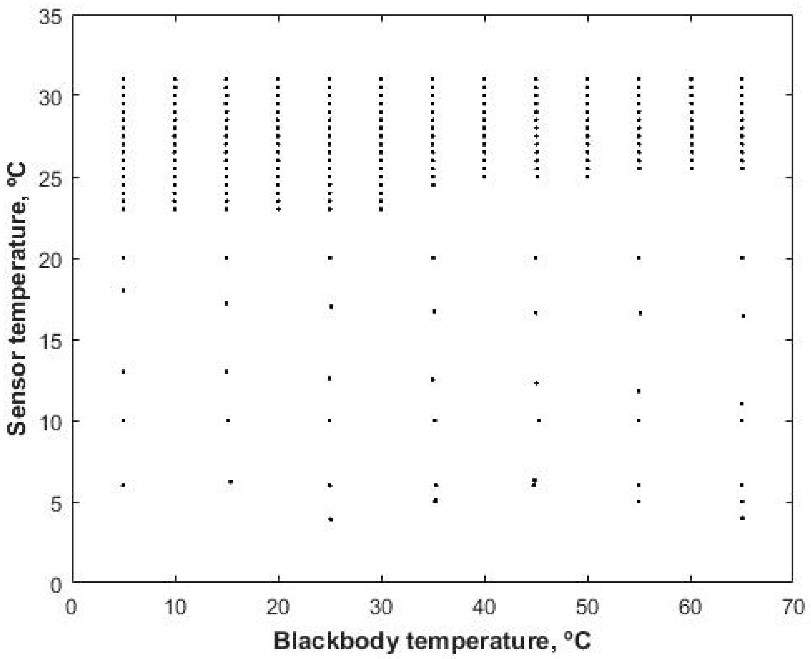
2.2. Radiometric Calibration Data Acquisition
2.3. Analyzed Algorithms for Radiometric Calibration
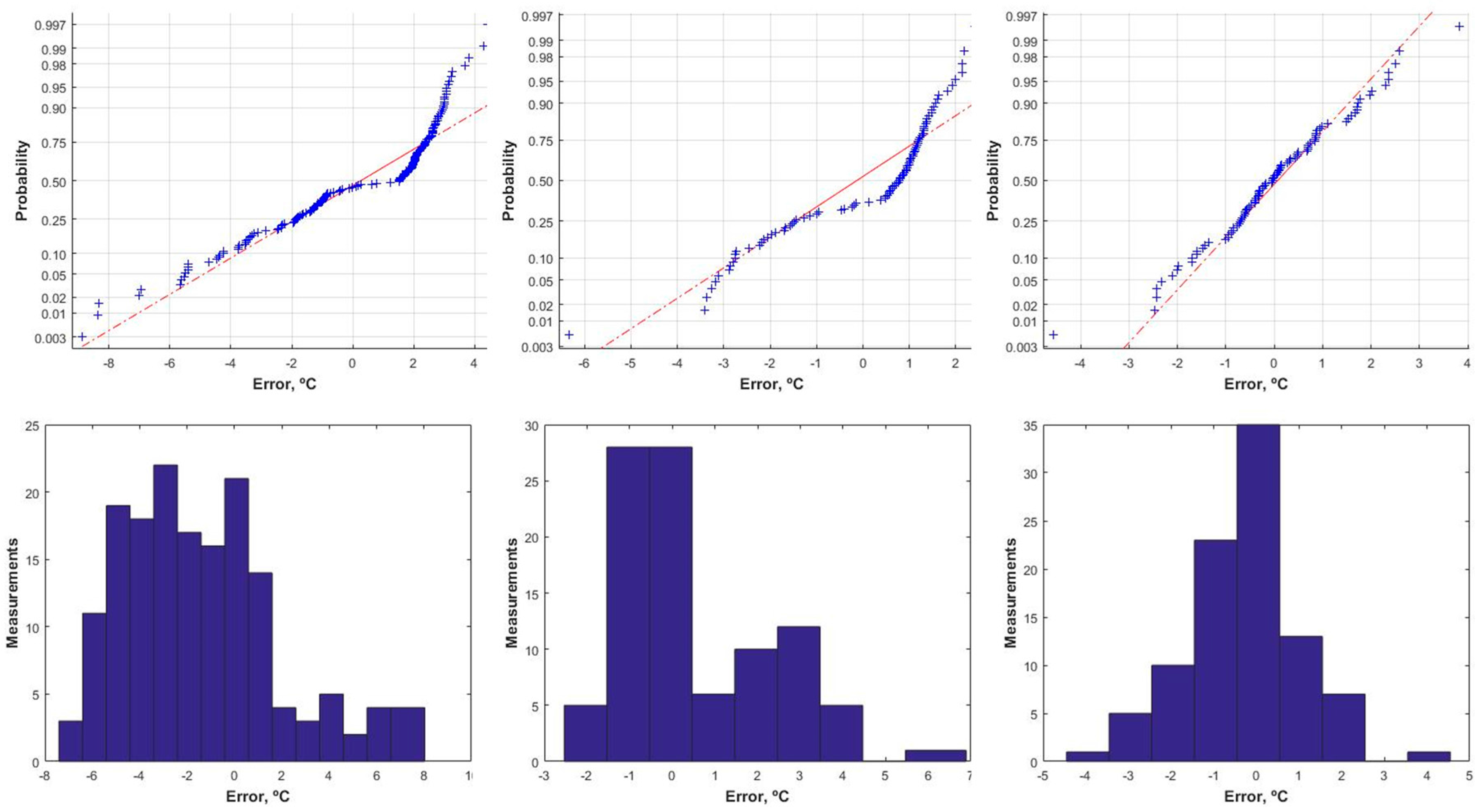
2.4. Analysis of Residuals
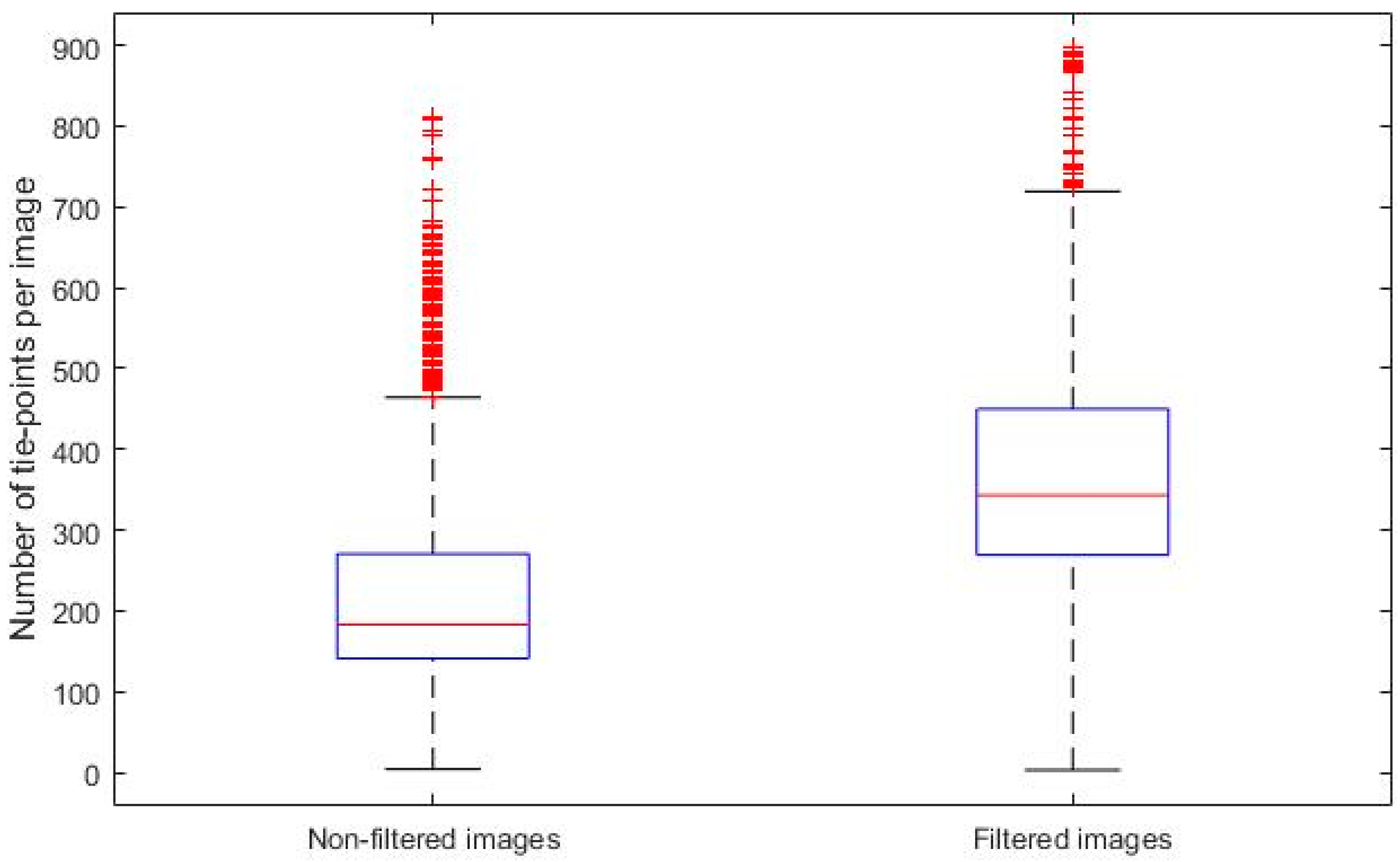
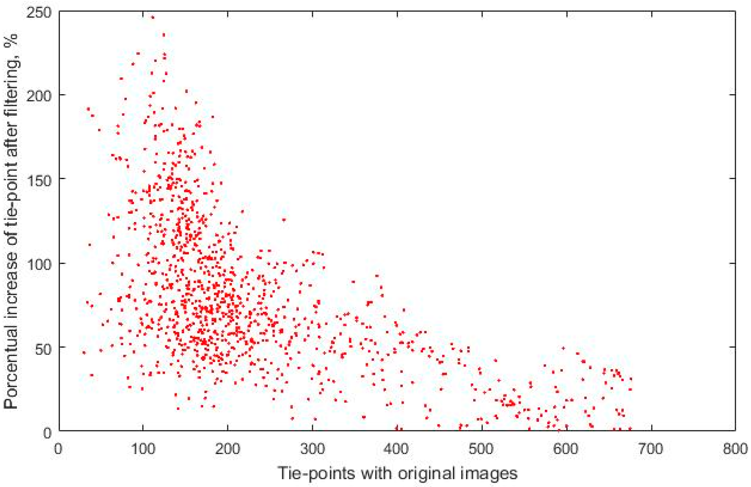
2.5. Photogrammetry Process and Image Filtering
- f: which is the focal length measured in pixels.
- cx and cy: which are the coordinates of the main point.
- b1, b2: which are the biased transformation coefficients.
- k1, k2, k3, k4: which are the radial distortion coefficients.
- p1, p2: which are the tangential distortion coefficients.
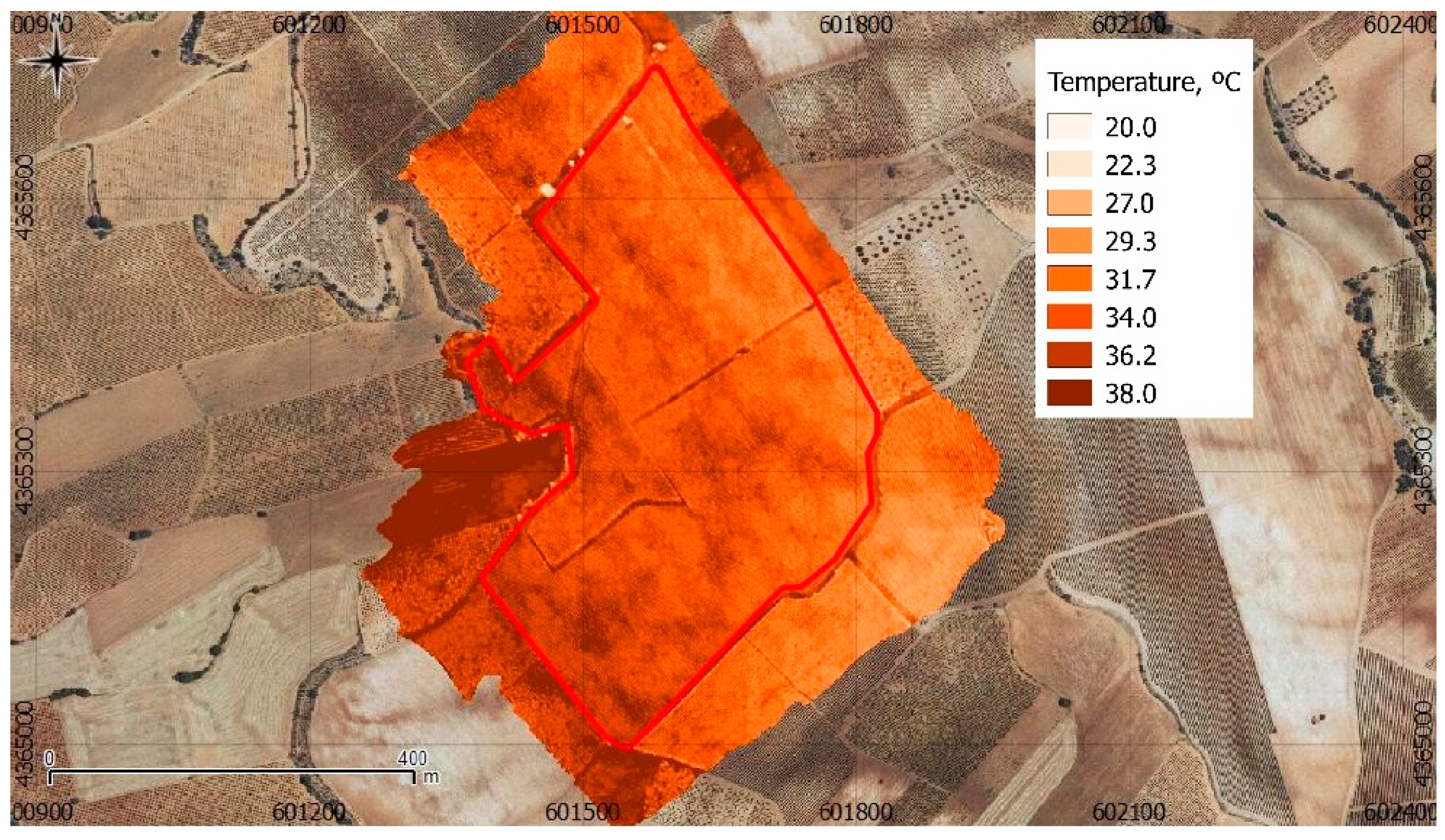
2.6. Application to a Case Study
2.7. Flight Planning and UAV Data Acquisition
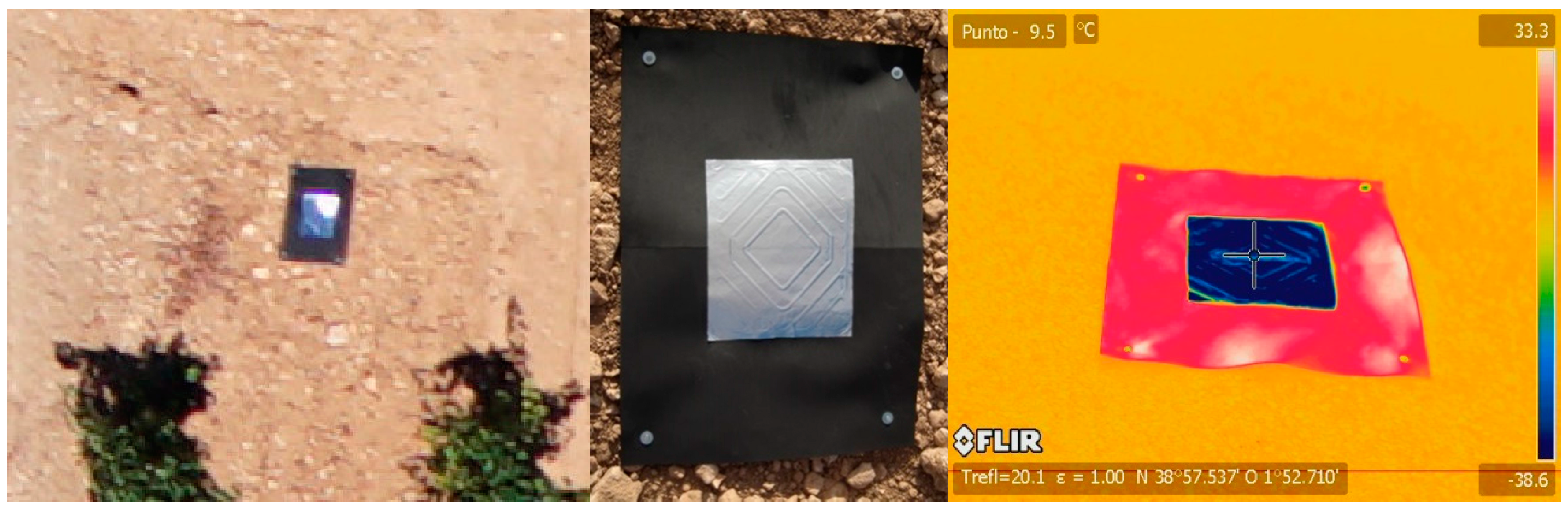
2.8. Ground Temperature Acquisition for Validation
3. Results
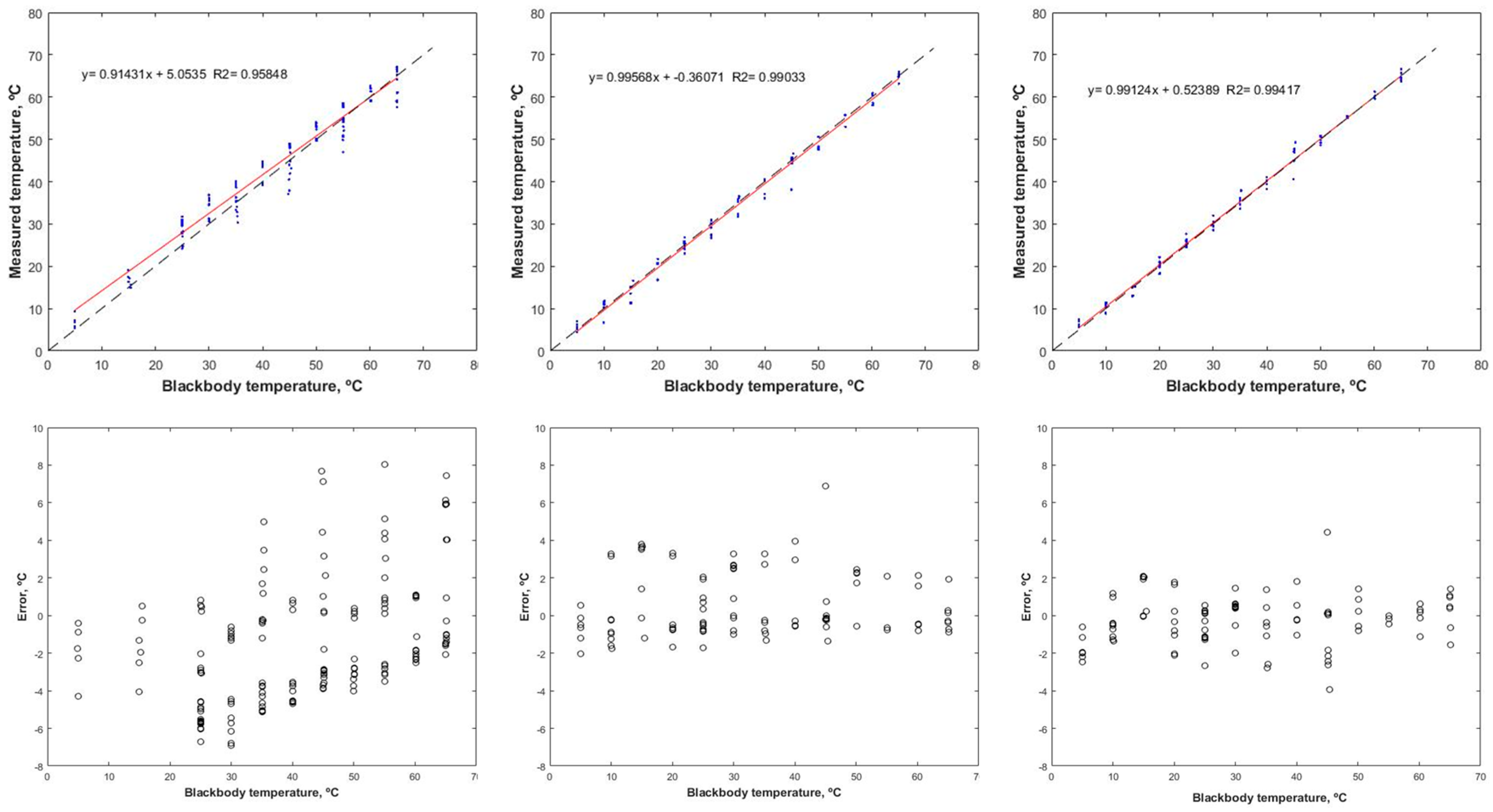
3.1. Error Analysis of the Uncooled Thermal Camera
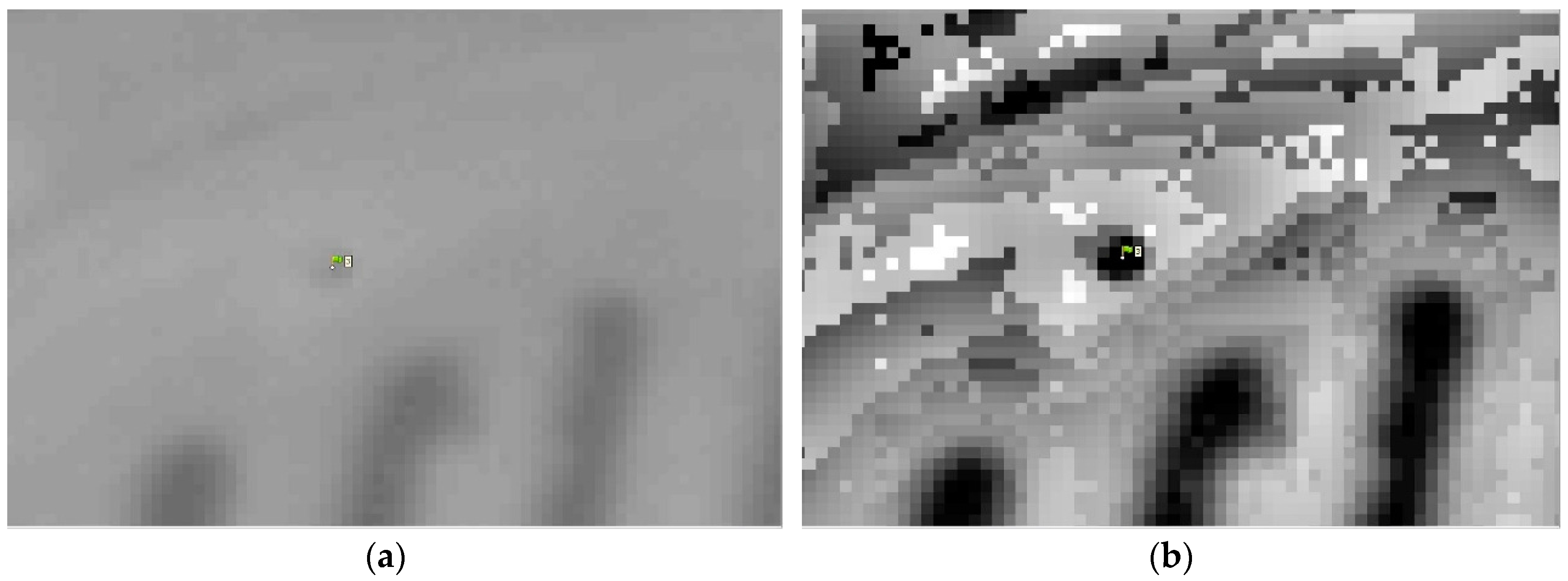
3.2. Results of Wallis Filter Application
3.3. Results of Temperature Measurements in the Case Study
4. Conclusions
Acknowledgments
Author Contributions
Conflicts of Interest
References
- Zhang, C.; Kovacs, J.M. The application of small unmanned aerial systems for precision agriculture: A review. Precis. Agric. 2012, 13, 693–712. [Google Scholar] [CrossRef]
- Ballesteros, R.; Ortega, J.F.; Hernández, D.; Moreno, M.A. Applications of georeferenced high-resolution images obtained with unmanned aerial vehicles. Part II: Application to maize and onion crops of a semi-arid region in Spain. Precis. Agric. 2014, 15, 593–614. [Google Scholar] [CrossRef]
- Laliberte, A.S.; Rango, A. Image Processing and Classification Procedures for Analysis of Sub-decimeter Imagery Acquired with an Unmanned Aircraft over Arid Rangelands. GISci. Remote Sens. 2011, 48, 4–23. [Google Scholar] [CrossRef]
- Majidi, B.; Bab-Hadiashar, A. Real time aerial natural image interpretation for autonomous ranger drone navigation. In Proceedings of the Digital Imag Computing Techniques and Application (DICTA 2005), Cairns, QLD, Australia, 6–8 December 2005; pp. 448–453. [Google Scholar]
- Berni, J.A.J.; Zarco-Tejada, P.J.; Suárez, L.; Fereres, E. Thermal and narrowband multispectral remote sensing for vegetation monitoring from an unmanned aerial vehicle. IEEE Trans. Geosci. Remote Sens. 2009, 47, 722–738. [Google Scholar] [CrossRef]
- Zarco-Tejada, P.J.; Berjón, A.; López-Lozano, R.; Miller, J.R.; Martín, P.; Cachorro, V.; González, M.R.; De Frutos, A. Assessing vineyard condition with hyperspectral indices: Leaf and canopy reflectance simulation in a row-structured discontinuous canopy. Remote Sens. Environ. 2005, 99, 271–287. [Google Scholar] [CrossRef]
- Kingston, D.B.; Beard, A.W. Real-time Attitude and Position Estimation for Small UAVs using Low-cost Sensors. In Proceedings of the AIAA 3rd Unmanned Unlimited Technical Conference on Workshop and Exhibit, Chicago, IL, USA, 20–23 September 2004. [Google Scholar]
- Ribeiro-Gomes, K.; Hernandez-Lopez, D.; Ballesteros, R.; Moreno, M.A. Approximate georeferencing and automatic blurred image detection to reduce the costs of UAV use in environmental and agricultural applications. Biosyst. Eng. 2016, 151, 308–327. [Google Scholar] [CrossRef]
- Baluja, J.; Diago, M.P.; Balda, P.; Zorer, R.; Meggio, F.; Morales, F.; Tardaguila, J. Assessment of vineyard water status variability by thermal and multispectral imagery using an unmanned aerial vehicle (UAV). Irrig. Sci. 2012, 30, 511–522. [Google Scholar] [CrossRef]
- Zaman-Allah, M.; Vergara, O.; Araus, J.L.; Tarekegne, A.; Magorokosho, C.; Zarco-Tejada, P.J.; Hornero, A.; Albà, A.H.; Das, B.; Craufurd, P.; et al. Unmanned aerial platform-based multi-spectral imaging for field phenotyping of maize. Plant Methods 2015, 11, 35. [Google Scholar] [CrossRef] [PubMed]
- Senthilnath, J.; Kandukuri, M.; Dokania, A.; Ramesh, K.N. Application of UAV imaging platform for vegetation analysis based on spectral-spatial methods. Comput. Electron. Agric. 2017, 140, 8–24. [Google Scholar] [CrossRef]
- Senthilnath, J.; Dokania, A.; Kandukuri, M.; Ramesh, K.N.; Anand, G.; Omkar, S.N. Detection of tomatoes using spectral-spatial methods in remotely sensed RGB images captured by UAV. Biosyst. Eng. 2016, 146, 16–32. [Google Scholar] [CrossRef]
- Bellvert, J.; Marsal, J.; Girona, J.; Zarco-Tejada, P.J. Seasonal evolution of crop water stress index in grapevine varieties determined with high-resolution remote sensing thermal imagery. Irrig. Sci. 2014, 33, 81–93. [Google Scholar] [CrossRef]
- Bellvert, J.; Zarco-Tejada, P.J.; Girona, J.; Fereres, E. Mapping crop water stress index in a “Pinot-noir” vineyard: Comparing ground measurements with thermal remote sensing imagery from an unmanned aerial vehicle. Precis. Agric. 2014, 15, 361–376. [Google Scholar] [CrossRef]
- Elvanidi, A.; Katsoulas, N.; Bartzanas, T.; Ferentinos, K.P.; Kittas, C. Crop water status assessment in controlled environment using crop reflectance and temperature measurements. Precis. Agric. 2017, 18, 332–349. [Google Scholar] [CrossRef]
- Ortega-Farías, S.; Ortega-Salazar, S.; Poblete, T.; Kilic, A.; Allen, R.; Poblete-Echeverría, C.; Ahumada-Orellana, L.; Zúñiga, M.; Sepúlveda, D. Estimation of energy balance components over a drip-irrigated olive orchard using thermal and multispectral cameras placed on a helicopter-based unmanned aerial vehicle (UAV). Remote Sens. 2016, 8, 638. [Google Scholar]
- Santesteban, L.G.; Di Gennaro, S.F.; Herrero-Langreo, A.; Miranda, C.; Royo, J.B.; Matese, A. High-resolution UAV-based thermal imaging to estimate the instantaneous and seasonal variability of plant water status within a vineyard. Agric. Water Manag. 2017, 183, 49–59. [Google Scholar] [CrossRef]
- Gómez-Candón, D.; Virlet, N.; Labbé, S.; Jolivot, A.; Regnard, J.L. Field phenotyping of water stress at tree scale by UAV-sensed imagery: New insights for thermal acquisition and calibration. Precis. Agric. 2016, 17, 786–800. [Google Scholar] [CrossRef]
- Rud, R.; Cohen, Y.; Alchanatis, V.; Levi, A.; Brikman, R.; Shenderey, C.; Heuer, B.; Markovitch, T.; Dar, Z.; Rosen, C.; et al. Crop water stress index derived from multi-year ground and aerial thermal images as an indicator of potato water status. Precis. Agric. 2014, 15, 273–289. [Google Scholar] [CrossRef]
- Möller, M.; Alchanatis, V.; Cohen, Y.; Meron, M.; Tsipris, J.; Naor, A.; Ostrovsky, V.; Sprintsin, M.; Cohen, S. Use of thermal and visible imagery for estimating crop water status of irrigated grapevine. J. Exp. Bot. 2007, 58, 827–838. [Google Scholar] [CrossRef] [PubMed]
- DeJonge, K.C.; Taghvaeian, S.; Trout, T.J.; Comas, L.H. Comparison of canopy temperature-based water stress indices for maize. Agric. Water Manag. 2015, 156, 51–62. [Google Scholar] [CrossRef]
- Allen, R.G.; Tasumi, M.; Morse, A.; Trezza, R.; Wright, J.L.; Bastiaanssen, W.; Kramber, W.; Lorite, I.; Robinson, C.W. Satellite-based energy balance for mapping evapotranspiration with internalized calibration (METRIC)—Applications. J. Irrig. Drain. Eng. 2007, 133, 395–406. [Google Scholar] [CrossRef]
- Bastiaanssen, W.G.M.; Menenti, M.; Feddes, R.A.; Holtslag, A.A.M. A remote sensing surface energy balance algorithm for land (SEBAL). 1. Formulation. J. Hydrol. 1998, 212, 198–212. [Google Scholar] [CrossRef]
- Gowda, P.H.; Chavez, J.L.; Colaizzi, P.D.; Evett, S.R.; Howell, T.A.; Tolk, J.A. ET mapping for agricultural water management: Present status and challenges. Irrig. Sci. 2008, 26, 223–237. [Google Scholar] [CrossRef]
- Roerink, G.J.; Su, Z.; Menenti, M. S-SEBI: A simple remote sensing algorithm to estimate the surface energy balance. Phys. Chem. Earth Part B Hydrol. Ocean. Atmos. 2000, 25, 147–157. [Google Scholar] [CrossRef]
- Norman, J.M.; Kustas, W.P.; Humes, K.S. Source approach for estimating soil and vegetation energy fluxes in observations of directional radiometric surface temperature. Agric. For. Meteorol. 1995, 77, 263–293. [Google Scholar] [CrossRef]
- Brenner, A.J.; Incoll, L.D. The effect of clumping and stomatal response on evaporation from sparsely vegetated shrublands. Agric. For. Meteorol. 1997, 84, 187–205. [Google Scholar] [CrossRef]
- Poblete-Echeverría, C.; Ortega-Farias, S. Estimation of actual evapotranspiration for a drip-irrigated merlot vineyard using a three-source model. Irrig. Sci. 2009, 28, 65–78. [Google Scholar] [CrossRef]
- Allen, R.; Irmak, A.; Trezza, R.; Hendrickx, J.M.H.; Bastiaanssen, W.; Kjaersgaard, J. Satellite-based ET estimation in agriculture using SEBAL and METRIC. Hydrol. Process. 2011, 25, 4011–4027. [Google Scholar] [CrossRef]
- Liou, Y.A.; Kar, S.K. Evapotranspiration estimation with remote sensing and various surface energy balance algorithms—A review. Energies 2014, 7, 2821–2849. [Google Scholar] [CrossRef]
- Su, Z. The Surface Energy Balance System (SEBS) for estimation of turbulent heat fluxes. Hydrol. Earth Syst. Sci. 2002, 6, 85–100. [Google Scholar] [CrossRef]
- Allen, R.G.; Tasumi, M.; Morse, A. Satellite-based evapotranspiration by METRIC and Landsat for western states water management. US Bur. Reclam. Evapotranspiration Workshop 2005, 1–19. [Google Scholar] [CrossRef]
- Ramos, J.G.; Cratchley, C.R.; Kay, J.A.; Casterad, M.A.; Martínez-Cob, A.; Domínguez, R. Evaluation of satellite evapotranspiration estimates using ground-meteorological data available for the Flumen District into the Ebro Valley of N.E. Spain. Agric. Water Manag. 2009, 96, 638–652. [Google Scholar] [CrossRef]
- Elhaddad, A.; Garcia, L.A.; Chavez, J.L. Using a surface energy balance model to calculate spatially distributed actual evapotranspiration. J. Irrig. Drain. Eng. 2011, 137, 17–26. [Google Scholar] [CrossRef]
- Poblete-Echeverría, C.; Ortega-Farias, S. Calibration and validation of a remote sensing algorithm to estimate energy balance components and daily actual evapotranspiration over a drip-irrigated Merlot vineyard. Irrig. Sci. 2012, 30, 537–553. [Google Scholar] [CrossRef]
- Allen, R.G.; Pereira, L.S.; Raes, D.; Smith, M. Crop Evapotranspiration: Guidelines for Computing Crop Requirements FAO Irrigation and Drainage Paper No. 56. FAO Rome 1998, 300, D05109. [Google Scholar]
- Awan, U.K.; Anwar, A.; Ahmad, W.; Hafeez, M. A methodology to estimate equity of canal water and groundwater use at different spatial and temporal scales: A geo-informatics approach. Environ. Earth Sci. 2016, 75, 1–13. [Google Scholar] [CrossRef]
- Mahmoud, S.H.; Alazba, A.A. A coupled remote sensing and the Surface Energy Balance based algorithms to estimate actual evapotranspiration over the western and southern regions of Saudi Arabia. J. Asian Earth Sci. 2016, 124, 269–283. [Google Scholar] [CrossRef]
- Idso, S.B.; Jackson, R.D.; Pinter, P.J.; Reginato, R.J.; Hatfield, J.L. Normalizing the stress-degree-day parameter for environmental variability. Agric. Meteorol. 1981, 24, 45–55. [Google Scholar] [CrossRef]
- King, B.A.; Shellie, K.C. Evaluation of neural network modeling to predict non-water-stressed leaf temperature in wine grape for calculation of crop water stress index. Agric. Water Manag. 2016, 167, 38–52. [Google Scholar] [CrossRef]
- Gade, R.; Moeslund, T.B. Thermal cameras and applications: A survey. Mach. Vis. Appl. 2014, 25, 245–262. [Google Scholar] [CrossRef]
- Sheng, H.; Chao, H.; Coopmans, C.; Han, J.; McKee, M.; Chen, Y. Low-cost UAV-based thermal infrared remote sensing: Platform, calibration and applications. In Proceedings of the 2010 IEEE/ASME International Conference on Mechatronic Embedded Systems and Applications (MESA), Qingdao, China, 15–17 July 2010; pp. 38–43. [Google Scholar]
- Jensen, A.M.; McKee, M.; Chen, Y. Procedures for processing thermal images using low-cost microbolometer cameras for small unmanned aerial systems. In Proceedings of the 2014 IEEE International Geoscience and Remote Sensing Symposium, Québec City, QC, Canada, 13–18 July 2014; pp. 2629–2632. [Google Scholar]
- Budzier, H.; Gerlach, G. Calibration of uncooled thermal infrared cameras. J. Sens. Sens. Syst. 2015, 4, 187–197. [Google Scholar] [CrossRef]
- Bishop, C.M. Neural networks for pattern recognition. J. Am. Stat. Assoc. 1995, 92, 482. [Google Scholar]
- Mcevoy, H.; Simpson, R.; Machin, G. Quantitative InfraRed Thermography Review of current thermal imaging temperature calibration and evaluation facilities, practices and procedures, across EURAMET. In Proceedings of the 11th International Conference on Quantitative InfraRed Thermography (QIRT 2012), Naples, Italy, 11–14 June 2012. [Google Scholar]
- Botterill, T.; Mills, S.; Green, R. Real-time aerial image mosaicing. In Proceedings of the International Conference Image and Vision Computing New Zealand, Queenstown, New Zealand, 8–9 November 2010; pp. 1–8. [Google Scholar]
- Ghosh, D.; Kaabouch, N. A survey on image mosaicing techniques. J. Vis. Commun. Image Represent. 2016, 34, 1–11. [Google Scholar] [CrossRef]
- Pierrot-Deseilligny, M.; Clery, I. Apero, an Open Source Bundle Adjusment Software for Automatic Calibration and Orientation of Set of Images. In Proceedings of the ISPRS Symposium, 3DARCH11, Trento, Italy, 2–4 March 2011. [Google Scholar]
- Wu, C. VisualSFM: A Visual Structure from Motion System. Available online: http://ccwu.me/vsfm/doc.html (accessed on 21 September 2017).
- Snavely, N.; Seitz, S.M.; Szeliski, R. Photo tourism: Exploring Photo Collections in 3D. ACM Trans. Graph. 2006, 25, 835–846. [Google Scholar] [CrossRef]
- Kastek, M.; Dulski, R.; Trzaskawka, P.; Bieszczad, G. Sniper detection using infrared camera: Technical possibilities and limitations. In SPIE Defense, Security, and Sensing; International Society for Optics and Photonics: Orlando, FL, USA, 2010. [Google Scholar]
- Hartmann, W.; Tilch, S.; Eisenbeiss, H.; Schindler, K. Determination of the Uav Position By Automatic Processing of Thermal Images. ISPRS-Int. Arch. Photogramm. Remote Sens. Spat. Inf. Sci. 2012, XXXIX-B6, 111–116. [Google Scholar] [CrossRef]
- Smoorenburg, M.; Volze, N.; Tilch, S.; Hartmann, W.; Naef, F.; Kinzelbach, W. Evaluation of Thermal Infrared Imagery Acquired with an Unmanned Aerial Vehicle for Studying Hydrological Processes. In Proceedings of the EGU General Assembly Conference Abstracts, Orlando, FL, USA, 5 May 2010. [Google Scholar]
- Pérez Álvarez, J.A. Apuntes de Fotogrametría II. Cent. Univ. Mérida 2001, 53, 1689–1699. [Google Scholar]
- Kou, F.; Chen, W.; Li, Z.; Wen, C. Content adaptive image detail enhancement. IEEE Signal Process. Lett. 2015, 22, 211–215. [Google Scholar] [CrossRef]
- Guidi, G.; Gonizzi, S.; Micoli, L.L. Image pre-processing for optimizing automated photogrammetry performances. ISPRS Ann. Photogramm. Remote Sens. Spat. Inf. Sci. 2014, II-5, 145–152. [Google Scholar] [CrossRef]
- Ballesteros, R.; Ortega, J.F.; Hernández, D.; Moreno, M.A. Applications of georeferenced high-resolution images obtained with unmanned aerial vehicles. Part I: Description of image acquisition and processing. Precis. Agric. 2014, 15, 593–614. [Google Scholar] [CrossRef]
- Wallis, K.F. Seasonal adjustment and relations between variables. J. Am. Stat. Assoc. 1974, 69, 18–31. [Google Scholar] [CrossRef]
- Gaiani, M.; Remondino, F.; Apollonio, F.I.; Ballabeni, A. An advanced pre-processing pipeline to improve automated photogrammetric reconstructions of architectural scenes. Remote Sens. 2016, 8, 178. [Google Scholar] [CrossRef]
- González-Aguilera, D.; López-Fernández, L.; Rodriguez-Gonzalvez, P.; Guerrero, D.; Hernandez-Lopez, D.; Remondino, F.; Menna, F.; Nocerino, E.; Toschi, I.; Ballabeni, A.; et al. Development of an all-purpose free photogrammetric tool. ISPRS Int. Arch. Photogramm. Remote Sens. Spat. Inf. Sci. 2016, 41, 31–38. [Google Scholar]
- Jazayeri, I.; Fraser, C. Interest operators in close-range object reconstruction. Int. Arch. Photogramm. Remote Sens. Spat. Inf. Sci. Beijing 2008, 37, 69–74. [Google Scholar]
- UNEP World Atlas of Desertification, 2nd ed.; Publications Office of the European Union: Luxembourg, 1997.
- Sánchez, J.M.; Kustas, W.P.; Caselles, V.; Anderson, M.C. Modelling surface energy fluxes over maize using a two-source patch model and radiometric soil and canopy temperature observations. Remote Sens. Environ. 2008, 112, 1130–1143. [Google Scholar] [CrossRef]
- Torres-Rua, A. Vicarious calibration of sUAS microbolometer temperature imagery for estimation of radiometric land surface temperature. Sensors 2017, 17, 1499. [Google Scholar] [CrossRef] [PubMed]


| Alignment Parameters | |
| Accuracy | High |
| Pair preselection | Generic |
| Key point limit | 40.000 |
| Tie point limit | 4.000 |
| Adaptive camera model fitting | yes |
| Optimized parameters | f, b1, b2, cx, cy, k1–k4, p1, p2 |
| Dense point cloud | |
| Quality | Medium |
| Depth filtering | Mild |
| Model | |
| Surface type | Arbitrary |
| Source data | Dense cloud |
| Face count | High |
| Interpolation | Enabled |
| Orthomosaic | |
| Mapping mode | Orthophoto |
| Blending mode | Mosaic |
| Manufacturer Configuration | Linear | P1 | P2 | P3 | P4 | ANN | |
|---|---|---|---|---|---|---|---|
| Data | 266 | 95 | 95 | 95 | 95 | 95 | 95 |
| R2 | 0.96 | 0.99 | 0.99 | 0.99 | 0.99 | 0.99 | 0.99 |
| RMSE, °C | 3.55 | 1.81 | 1.81 | 1.49 | 1.51 | 1.51 | 1.37 |
| Relative Error, % | 8.47 | 5.59 | 5.57 | 4.59 | 4.66 | 4.66 | 4.22 |
| Similarity Index | 0.99 | 1.00 | 1.00 | 1.00 | 1.00 | 1.00 | 1.00 |
| Unfiltered Images | Filtered Images | |
|---|---|---|
| Number of images | 1154 | 1154 |
| Flight height (m) | 81.1 | 80.4 |
| Ground resolution (cm pix−1) | 13.8 | 13.5 |
| Covered area (km2) | 0.366 | 0.364 |
| Number of images oriented | 1.148 | 1.151 |
| Tie-points | 58,193 | 110,089 |
| Projections | 272,078 | 445,291 |
| Re-projection error (pix) | 0.504 | 0.442 |
| GCP | Error X (mm) | Error Y (mm) | Error Z (mm) | Total (mm) | Image (pix) |
|---|---|---|---|---|---|
| 1 | 1.00 | −1.12 | 0.80 | 1.70 | 0.58 (34) |
| 2 | −3.81 | −0.33 | 2.78 | 4.73 | 0.97 (49) |
| 3 | 4.82 | 1.65 | −10.87 | 12.01 | 0.74 (32) |
| 4 | 2.69 | 1.41 | 5.83 | 6.57 | 0.65 (30) |
| 5 | 0.53 | 3.56 | 2.36 | 4.30 | 0.36 (32) |
| 7 | −2.41 | −5.36 | −6.14 | 8.50 | 0.56 (26) |
| 8 | −1.60 | 0.68 | 4.89 | 5.19 | 0.86 (24) |
| 9 | −1.48 | 0.33 | −8.92 | 9.05 | 0.53 (31) |
| Total | 2.66 | 2.45 | 6.20 | 7.18 | 0.70 |
| GCP | Error X (mm) | Error Y (mm) | Error Z (mm) | Total (mm) | Image (pix) |
|---|---|---|---|---|---|
| 1 | −0.37 | 0.46 | −0.98 | 1.14 | 0.57 (34) |
| 2 | −0.19 | −0.24 | −0.04 | 0.32 | 1.65 (49) |
| 3 | 0.02 | 0.32 | 0.13 | 0.35 | 0.64 (31) |
| 4 | 0.05 | −0.64 | 1.33 | 1.48 | 0.87 (32) |
| 5 | 1.32 | 0.61 | 1.00 | 1.77 | 0.38 (32) |
| 7 | −0.98 | −0.32 | −1.78 | 2.05 | 0.67 (27) |
| 8 | −0.20 | 0.28 | 0.90 | 0.97 | 0.78 (23) |
| 9 | 0.08 | −0.39 | −0.17 | 0.43 | 0.51 (31) |
| Total | 0.61 | 0.43 | 0.98 | 1.23 | 0.92 |
| Handheld Camera | Original Configuration | Corrected Data | ||||
|---|---|---|---|---|---|---|
| Mean | SD | Mean | SD | Mean | SD | |
| RV 1 | 30.2 | 0.3 | 32.0 | 0.1 | 29.7 | 0.1 |
| RV 2 | 29.2 | 0.2 | 33.8 | 0.0 | 31.7 | 0.1 |
| RV 3 | 27.7 | 0.3 | 33.8 | 0.2 | 31.6 | 0.2 |
| RV 4 | 29.3 | 0.3 | 32.7 | 0.4 | 30.5 | 0.4 |
| RV 5 | 29.2 | 0.3 | 31.4 | 0.1 | 29.1 | 0.2 |
| IV 1 | 27.4 | 0.1 | 28.3 | 0.0 | 25.8 | 0.0 |
| IV 2 | 26.8 | 0.3 | 28.2 | 0.3 | 25.6 | 0.3 |
| IV 3 | 28.6 | 0.2 | 27.2 | 0.0 | 24.6 | 0.0 |
| IV 4 | 27.4 | 0.2 | 28.1 | 0.5 | 25.5 | 0.5 |
| IV 5 | 26.0 | 0.2 | 28.5 | 0.3 | 26.0 | 0.3 |
| 7d-IV 1 | 28.2 | 0.3 | 33.4 | 0.0 | 31.4 | 0.0 |
| 7d-IV 2 | 26.7 | 0.3 | 32.7 | 0.3 | 30.6 | 0.3 |
| 7d-IV 3 | 28.3 | 0.1 | 32.5 | 0.2 | 30.4 | 0.2 |
| 7d-IV 4 | 27.1 | 0.1 | 31.4 | 0.1 | 29.3 | 0.1 |
| 7d-IV 5 | 28.3 | 0.1 | 30.9 | 0.0 | 28.8 | 0.0 |
| Soil 1 | 42.8 | 0.2 | 42.2 | 0.1 | 40.7 | 0.1 |
| Soil 2 | 42.3 | 0.3 | 41.6 | 0.1 | 40.1 | 0.1 |
| Soil 3 | 41.7 | 0.3 | 40.6 | 0.1 | 39.0 | 0.1 |
| Soil 4 | 43.2 | 0.5 | 40.1 | 0.1 | 38.4 | 0.1 |
| Soil 5 | 41.3 | 0.2 | 39.2 | 0.0 | 37.5 | 0.0 |
© 2017 by the authors. Licensee MDPI, Basel, Switzerland. This article is an open access article distributed under the terms and conditions of the Creative Commons Attribution (CC BY) license (http://creativecommons.org/licenses/by/4.0/).
Share and Cite
Ribeiro-Gomes, K.; Hernández-López, D.; Ortega, J.F.; Ballesteros, R.; Poblete, T.; Moreno, M.A. Uncooled Thermal Camera Calibration and Optimization of the Photogrammetry Process for UAV Applications in Agriculture. Sensors 2017, 17, 2173. https://doi.org/10.3390/s17102173
Ribeiro-Gomes K, Hernández-López D, Ortega JF, Ballesteros R, Poblete T, Moreno MA. Uncooled Thermal Camera Calibration and Optimization of the Photogrammetry Process for UAV Applications in Agriculture. Sensors. 2017; 17(10):2173. https://doi.org/10.3390/s17102173
Chicago/Turabian StyleRibeiro-Gomes, Krishna, David Hernández-López, José F. Ortega, Rocío Ballesteros, Tomás Poblete, and Miguel A. Moreno. 2017. "Uncooled Thermal Camera Calibration and Optimization of the Photogrammetry Process for UAV Applications in Agriculture" Sensors 17, no. 10: 2173. https://doi.org/10.3390/s17102173
APA StyleRibeiro-Gomes, K., Hernández-López, D., Ortega, J. F., Ballesteros, R., Poblete, T., & Moreno, M. A. (2017). Uncooled Thermal Camera Calibration and Optimization of the Photogrammetry Process for UAV Applications in Agriculture. Sensors, 17(10), 2173. https://doi.org/10.3390/s17102173