3.1. Impedance Response
Impedance measurements were carried out in order to determine the effect of electrode configuration on the electrical response of the NO
x sensors.
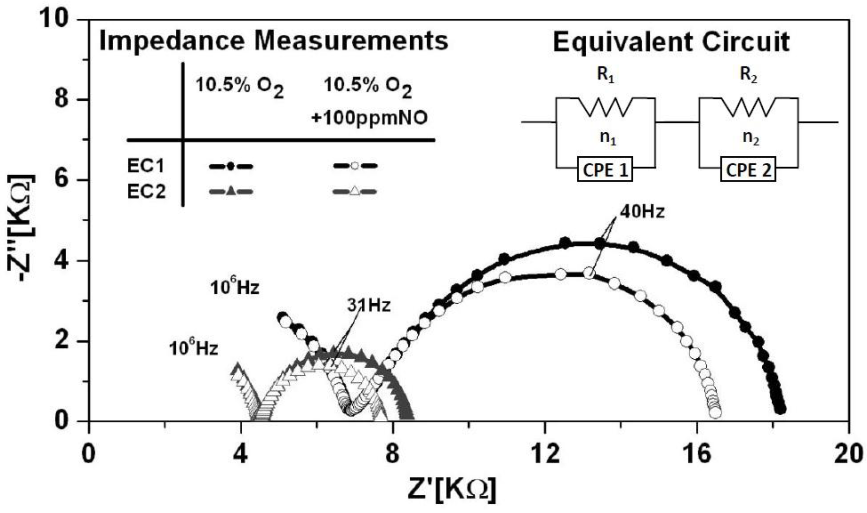
Figure 2 shows typical impedance data collected for EC1 and EC2 sensors at an operating temperature of 650 °C in the presence of 10.5% O
2 with and without 100 ppm NO. The impedance response for 100 ppm NO
2 was very similar to the response measured for 100 ppm NO. Similar results were observed in previous studies [
9]. Thermodynamic conversion of NO
2 to NO causes the vast majority (over 90%) of NO
2 to convert to NO at temperatures over 600 °C. Thus, data presented here concentrates on the NO response. The data was measured in triplicate for each testing condition to insure that stable, reproducible data was collected. The impedance data indicated two distinct arcs for both the EC1 and EC2 sensors. The incomplete high frequency arc (HFA) resulted from the frequency limit of the Gamry Reference 600. Bulk electrolyte properties associated with the porous YSZ microstructure, such as oxygen ion conductivity are described by the high frequency response. More importantly, the impedancemetric NO
x sensor response is primarily described by electrode reactions, which are presented in the low frequency regime. The impedance response for EC1 sensors with the Au wire loop and embedded electrodes was substantially larger than the response of the EC2 sensors with parallel Au wire electrodes. In general, the impedance response of NO
x sensors depends upon the material properties, molecular and electronic transport, as well as the following electrochemical reduction/oxidation reactions:
These reactions occur along the triple phase boundary (TPB) where the electrode, electrolyte and gas species come into contact with each another. The low frequency impedance response is influenced by TPB Reactions (1) and (2) [
6,
7]. Since the sensors are composed of the same materials, it is likely that similar reactions occurred at each sensor. However, the pathways associated with those reactions may have differed. The tortuous microstructure of the porous electrolyte and, in particular, the distance between the electrodes affects the molecular and ionic transport within the sensors.
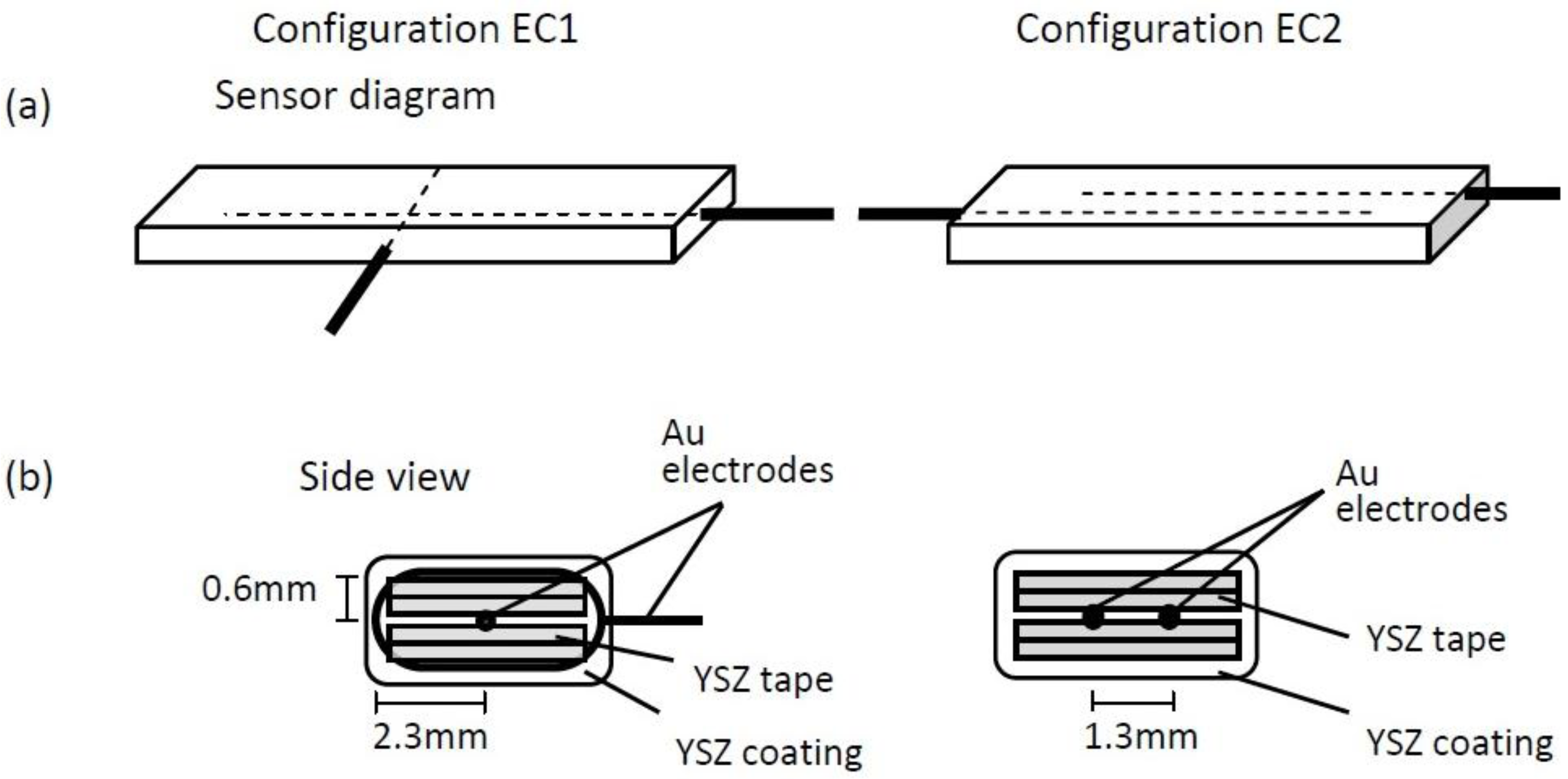
Figure 1 shows the distance between the wire loop and embedded electrodes in the EC1 sensors varied from approximately 0.6–2.3 mm; whereas, the parallel electrodes for EC2 sensors were about 1.3 mm apart. The variation in distance between the electrodes within EC1 sensors caused NO
x and O
2 gas species, as well as oxygen ions to travel longer distances through the tortuous pathways of the porous electrolyte in order to participate in TPB reactions. Similar observations have been made in solid oxide fuel cell (SOFC) studies where larger impedance measurements are reported for SOFCs composed of a thick film
versus thin film electrolyte. [
14,
15] The thick film electrolyte results in a greater distance between the electrodes, thereby, creating a longer pathway for oxygen ion transport through the electrolyte. As a result greater ohmic losses occur, which contribute to higher impedance values. Thus, the longer pathways for gas and oxygen ion transport within the EC1 sensors most likely contributed to the larger impedance.
Equivalent circuit modeling with Gamry EIS300 software was used to simulate the impedance measurements and further analyze the electrical response of the sensors under various operating conditions. The equivalent circuit model that best fit the sensor impedance results was, (R
1CPE
1) (R
2CPE
2), as shown in
Figure 2 for both sensor configurations. The resistor, R
1, was associated with the HFA and interpreted as the ionic transport resistance of the porous YSZ electrolyte. Other studies have shown that the HFA dependents upon the porosity of the electrolyte as the tortuous pathways within the porous microstructure impede the flow of oxygen ions [
9,
16]. The low frequency arc (LFA) resistance, R
2, described the interfacial resistance associated with TPB reactions. Such reactions include adsorption, dissociation, and diffusion of gases, as well as charge transfer, which can contribute to the electrode resistance. Further details on electrode reactions are discussed in follow sections. The equivalent circuit model accounted for the slight suppression of the arcs with constant phase elements, CPE
1 and CPE
2, which described the non-ideal capacitance behavior of the electrolyte and electrodes, respectively. Surface defects, interfacial reactions, as well as the morphology of the sensor components, can cause the time constant for various reactions to differ resulting in non-ideal capacitance behavior [
6].
Table 1 shows the fitted values associated with the equivalent circuit model shown in
Figure 2. The goodness of fit (
i.e., Chi squared) describes the quality of the fit. The errors associated with the fitting parameters were 1%–4% and 5%–6% where the goodness of fit was on the order of 10
−6 and 10
−4, respectively. The impedance data collected under the various operating conditions were fit using the same model and had goodness of fit values within this range.
Figure 2.
Typical Nyquist plot showing the impedance response of EC1 and EC2 sensors at an operating temperature of 650 °C, in 10.5% O2 with and without NO present. The equivalent circuit used to model the data is shown in the upper right corner of the plot. The model that fit the data is described by the solid lines.
Table 1.
Equivalent circuit fitting parameters are shown for sensor impedance data collected at 650 °C.
Table 1.
Equivalent circuit fitting parameters are shown for sensor impedance data collected at 650 °C.
| Sensor | High Frequency Arc | Low Frequency Arc | Goodness of Fit |
|---|
| 10.5% O2 | 10.5% O2 | 10.5% O2 + 100 ppm NO |
|---|
| CPE1 (F) | n1 | R1 (kΩ) | CPE2 (F) | n2 | R2 (kΩ) | CPE2 (F) | n2 | R2 (kΩ) |
|---|
| EC1 | 1.11 × 10⁻¹⁰ | 0.9 | 7.01 | 0.92 × 10⁻⁶ | 0.8 | 11.65 | 0.89 × 10⁻⁶ | 0.9 | 9.87 | 2.10 × 10⁻⁴ |
| EC2 | 0.75 × 10⁻¹⁰ | 0.9 | 4.54 | 2.22 × 10⁻⁶ | 0.9 | 3.90 | 2.24 × 10⁻⁶ | 0.9 | 3.23 | 2.90 × 10⁻⁶ |
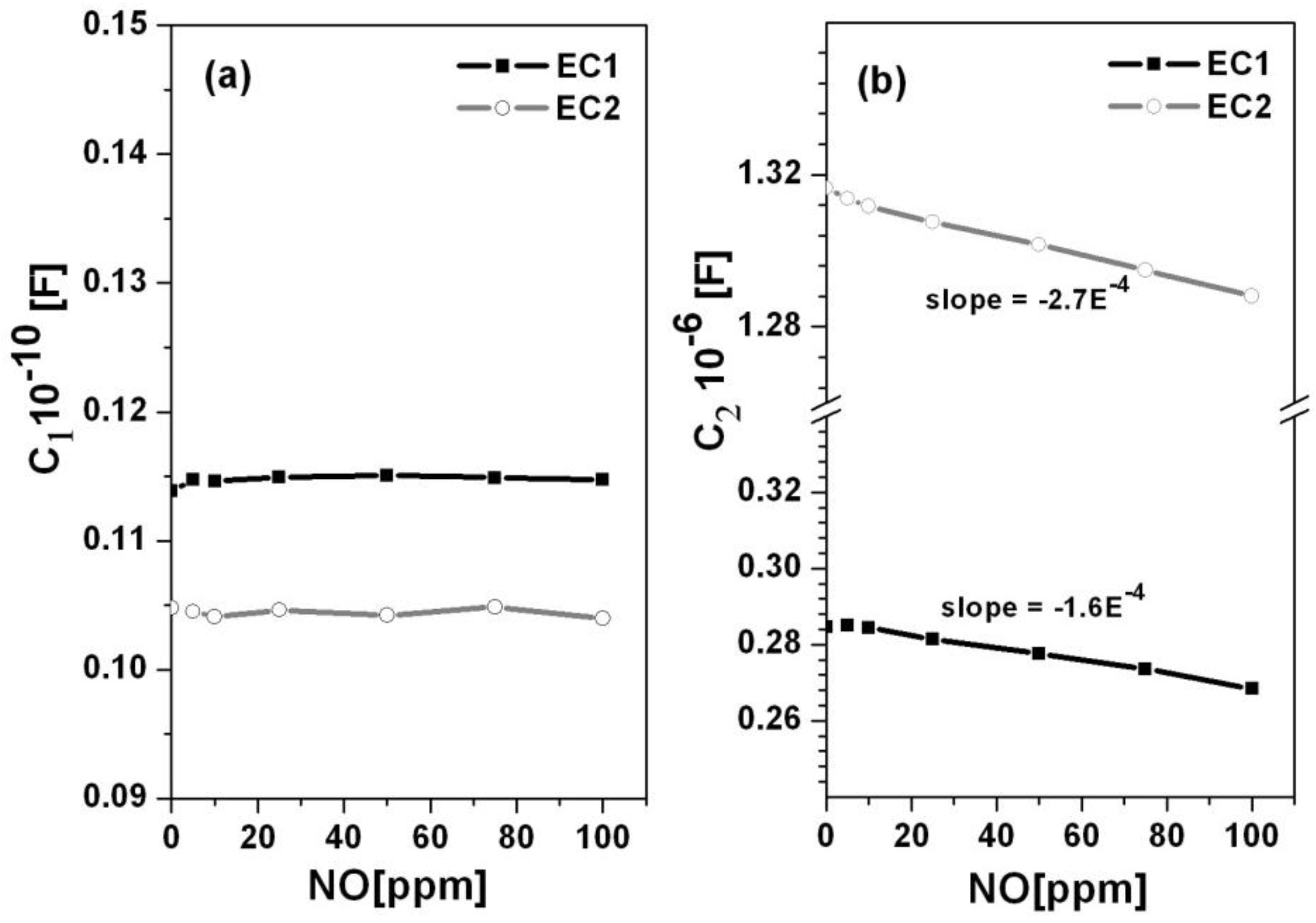
The fitted values for the CPE data generated for EC1 and EC2 sensors were used to calculate the capacitance, C, associated with the high and low frequency sensor response according to the following equation:
where R was the resistance associated with the low frequency impedance arc, and
n describes the deviation from pure capacitance behavior. In the case where
n = 1, the constant phase element represents a pure capacitor.
Figure 3 shows the capacitances, C1 and C2, with respect to NO concentration for the EC1 and EC2 sensors, respectively. The EC2 sensors had higher capacitance values in comparison to the EC1 sensors. Higher capacitance has been associated with increased oxygen coverage at the Au/YSZ interface [
17]. If oxygen arrived at this interface faster than it could participate in TPB reactions, then the shorter path length between the embedded parallel electrodes in the EC2 sensors may have enabled oxygen accumulation at the Au/YSZ interface. As for the EC1 sensors, the greater distance between the wire loop and embedded electrodes may have caused oxygen transport to occur over a longer time period such that the rate of oxygen arriving at the Au/YSZ interface coincided more closely with TPB reaction rates. In such a case, oxygen arriving at the Au/YSZ interface would more immediately participated in interfacial reactions, such that limited accumulation occurred. This suggests that the rate of oxygen transport through the porous YSZ electrolyte in EC1 sensors agreed more closely with the rate of interfacial reactions. The data in
Figure 3 also indicates that as the concentration of NO increased, the capacitance decreased, which suggests that oxygen coverage diminished as NO occupied more sites along the TPB.
Figure 3.
The capacitance versus NO concentration is shown for the (a) high and (b) low frequency arcs associated with the EC1 and EC2 sensors.
Figure 3.
The capacitance versus NO concentration is shown for the (a) high and (b) low frequency arcs associated with the EC1 and EC2 sensors.
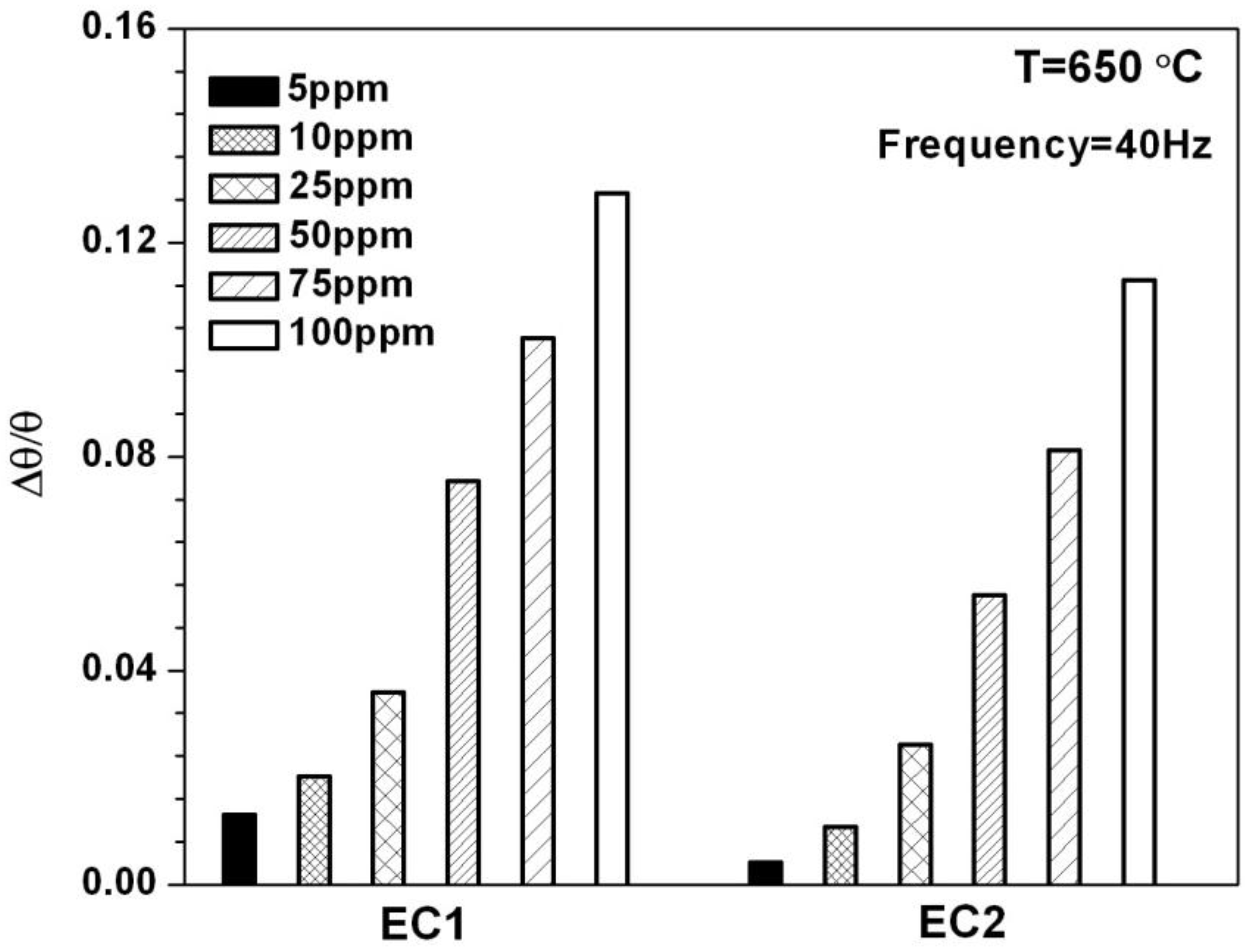
3.2. NO Sensitivity
Various methods have been used to assess NO sensor sensitivity. The operating conditions as well as material properties of the sensor components can significantly influence the degree of sensitivity observed by a given method. [
18]
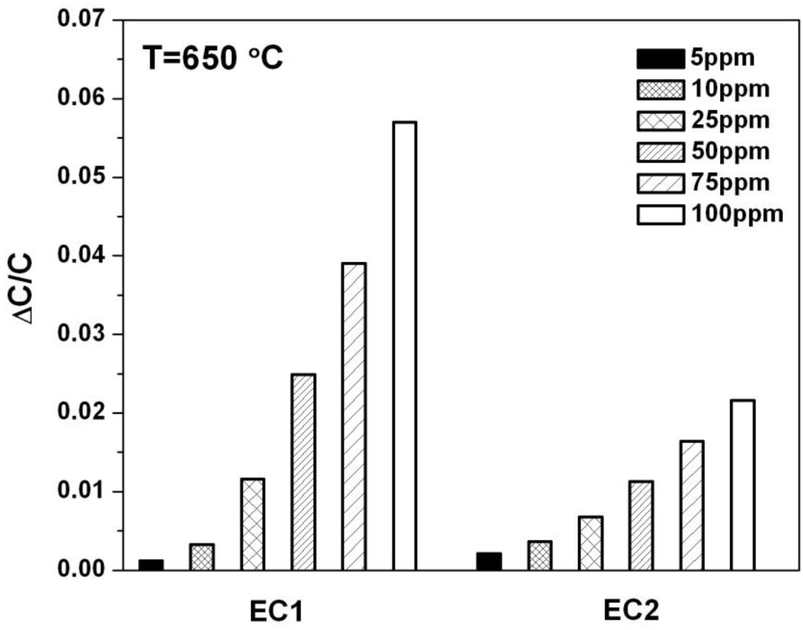
Figure 4 shows NO sensitivity for EC1 and EC2 sensors in terms of the change in capacitance,
, where
[
19]. The terms C
O2 and C
NO were the capacitance values calculated from fitted data for the LFAs according to Equation (3). C
O2 was the baseline capacitance that was determined when only 10.5% O
2 was exposed to the sensor. The capacitance, C
NO, was calculated based on the presence of a specific concentration of NO in the gas surrounding the sensor. The data in
Figure 4, indicates the sensitivity to NO was significantly greater for EC1
versus EC2 sensors. These findings along with the capacitance data in
Figure 3 suggest that lower oxygen coverage at the electrode/electrolyte interface in EC1 sensors may have allowed more NO reactions to take place at the TPB, which contributed to greater NO sensitivity.
Figure 4.
The change in capacitance is plotted for EC1 and EC2 sensors for NO concentrations ranging from 5 to 100 ppm.
Figure 4.
The change in capacitance is plotted for EC1 and EC2 sensors for NO concentrations ranging from 5 to 100 ppm.
The phase angle
θ, is a frequency dependent parameter that also can be used to evaluate the impedancemetric NOx sensor response. The relationship between the phase angle and the impedance is given by the equation
, where
and
are the imaginary and real components of the impedance, respectively. NO sensitivity can be determined by calculating the percent change in the phase angle response,
, for a specific operating frequency when the sensor is exposed to NO. The percent change in phase is defined as
, where
θO2 represented the baseline phase when only 10.5% O
2 was present and
θNO described the phase response for a specific concentration of NO.
Figure 5 shows the NO sensitivity for EC1 and EC2 sensors based on the phase response at 40 Hz. This data agrees with the sensitivity data presented in
Figure 4, as EC1 sensors demonstrated greater NO sensitivity in comparison to EC2 sensors. Further comparison between
Figure 4 and
Figure 5 indicates NO sensitivity based on
is greater than the sensitivity associated with
, particularly for the EC2 sensors. The phase response data also shows a higher sensitivity at lower NO concentrations, specifically 5 and 10 ppm. It is important to note that NO sensitivity based on
is dependent upon the sensor operating frequency. In general, the higher the operating frequency the more rapid the sensor response becomes to changes in NO concentration; however, NO sensitivity generally decreasing as the operating frequency increases. In this study, the
data collected at 40 Hz was determined to be the most suitable operating frequency with respect to such tradeoffs.
Figure 5.
The change in the angular phase angle is plotted for EC1 and EC2 sensors for NO concentrations ranging from 5 to 100 ppm.
Figure 5.
The change in the angular phase angle is plotted for EC1 and EC2 sensors for NO concentrations ranging from 5 to 100 ppm.
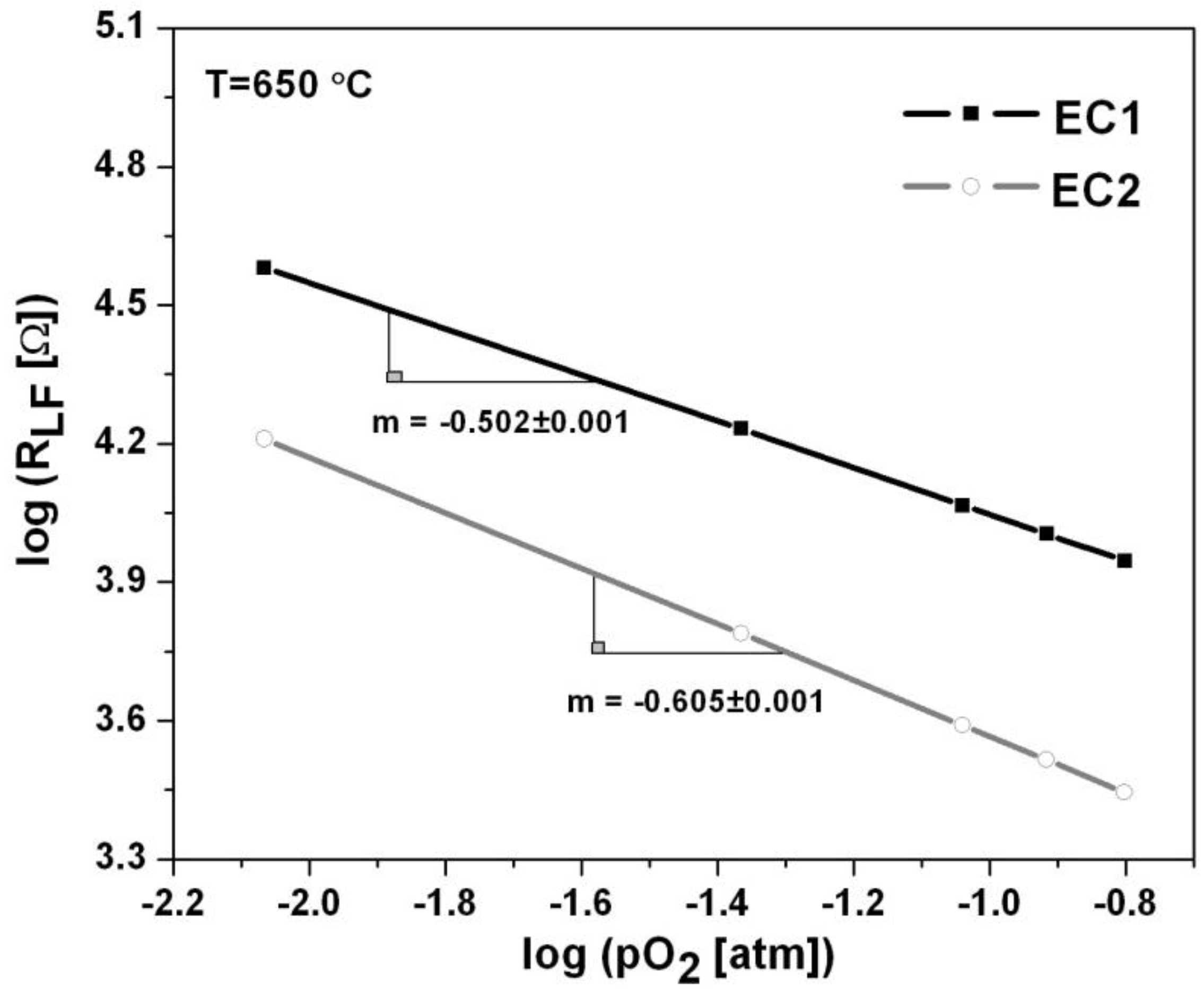
3.3. Oxygen and Temperature Dependence
The oxygen partial pressure and temperature dependence of the sensors can further understanding of potential rate limiting mechanisms and kinetic reactions that influence sensor behavior. The oxygen partial pressure dependence was determined for the low frequency arcs associated with the EC1 and EC2 sensors according to the power law relationship,
, where the slope, m, describes the rate limiting step. As shown in
Figure 6, a dependence of
and
was observed for EC1 and EC2 sensors, respectively. Studies concerning oxygen partial pressure dependence have reported that slope values corresponding to −0.5 indicate electrode surface reactions involving dissociative adsorption or atomic diffusion of oxygen as the rate limiting mechanism [
20]. As the slope becomes closer to −1 gas diffusion has been considered as rate limiting [
20]. The more negative slope dependence, m = −0.62, for the EC2 sensors seems to suggest gas diffusion contributed to the rate limiting steps. It is possible that the diffusion depth to the electrode/electrolyte interface within the EC2 sensors limited gas diffusion. The EC2 sensors were composed of parallel electrodes that were embedded approximately 0.75 mm within in the electrolyte; whereas, the wire loop electrode around the EC1 sensors had a thin electrolyte coating of about 0.15 mm in thickness. Thus, O
2 and NO gases traveled a shorter path to a TPB within the EC1 sensors, in comparison to EC2 sensors where the diffusion depth was greater.
Figure 6.
The oxygen partial pressure dependence of the EC1 and EC2 sensors is shown for data collected at 650 °C for oxygen concentrations ranging from 1% to 18%.
Figure 6.
The oxygen partial pressure dependence of the EC1 and EC2 sensors is shown for data collected at 650 °C for oxygen concentrations ranging from 1% to 18%.
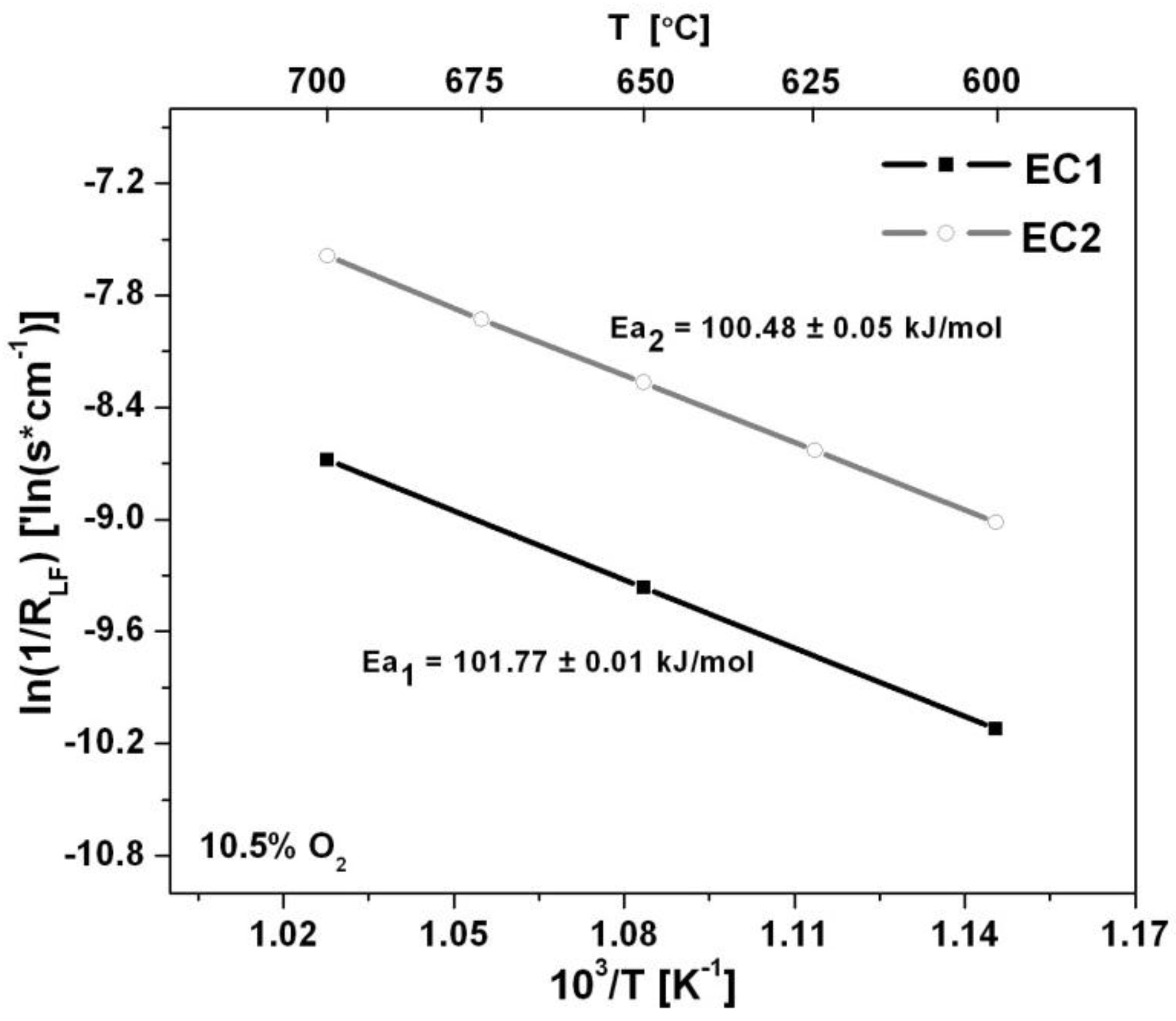
Arrhenius plots shown in
Figure 7 describe the temperature dependence of the sensors. The activation energies calculated from the slope of the Arrhenius plots were very similar for each electrode configuration as Ea
1 = 101.77 ± 0.01 kJ/mol and Ea
2 = 100.48 ± 0.05 kJ/mol for EC1 and EC2 sensors, respectively. The activation energy describes the temperature dependence of the electrode/electrolyte system. As the operating temperature increased the activation energy decreased suggesting that interfacial reactions were able to proceed more readily. The similar behavior described by the activation energy for the EC1 and EC2 sensors indicates a negligible relationship between the electrode configuration and temperature dependence of the sensors.
Figure 7.
The temperature dependence is described by the Arrhenius plot for the EC1 and EC2 sensors along with corresponding activation energies.
Figure 7.
The temperature dependence is described by the Arrhenius plot for the EC1 and EC2 sensors along with corresponding activation energies.


