1. Introduction
Recent years there have been a lot of applications in Wireless Sensor Networks (WSNs), ranging from monitoring to event detection and target tracking. For all these applications, data gathering is one of the primary operations carried out in WSNs [
1,
2,
3,
4]. Traditionally, the network is assumed to be dense so that there are end-to-end multi-hop paths within the network, along which the generated data could be routed to the base station. This assumption, however, does not always hold in the scenarios of real network deployments. For example, as the WSN is often deployed in harsh environments, the signal is susceptible to external interference and leads to disconnected and portioned network; and if the network is sparse or the nodes are mobile, the paths to the sink might not always be available. So recently there is a research trend that adopts mobile elements for the message transmission and data gathering in mobile sensor networks [
5,
6].
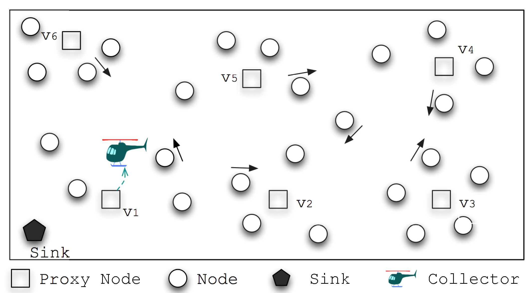
In these schemes mobile data collectors, e.g., autonomous robots, are used to move within the sensing field, collects data from sensor nodes and brings them to the sink. The ordinary nodes, on the other hand, just stay stationary and wait for the mobile data collector to come and pick up the data. So the
funnelling effect [
7], where the energy of nodes near the sink is depleted quickly because of forwarding more data packets than nodes distant from the sink, could be avoided. Mobile elements also make data gathering in a sparse or disconnected network possible because the collector can travel and directly collect the data from sensors. One strategy of data gathering with mobile elements is to map the data gathering problem into the optimization of trajectories of the mobile collector, and various scheduling schemes are proposed to increase the network lifetime or to minimize the traveling distance of mobile elements [
1,
3,
4,
6,
8,
9,
10]. In these schemes, however, ordinary nodes should be stationary and there should be paths or tracks available among the nodes, which are not always true in network deployments. Another strategy [
11,
12,
13,
14] is to adopt an opportunistic “Store-Carry-Forward” routing protocols, the same as those in the Delay-Tolerant Networks [
15,
16], for data gathering when both the ordinary nodes and data collector are mobile. Because both the ordinary nodes and the collector are mobile, there is no stable trajectories along which the collector could move within the network for data gathering, neither are the static links between the source node and the collector. So a
flooding or
epidemic approach is usually adopted for the message routing, which leads to unnecessary transmissions and energy depletion of nodes.
In this paper, we study the problem of data gathering in mobile sensor networks with speedy mobile elements, especially when there is no predefined paths or tracks for the data collector. For example, an autonomous underwater vehicle is used as a mobile sink to gather data from a randomly distributed underwater sensor network [
17]; in the wildlife monitoring application [
11], sensor nodes are attached to the monitoring targets so that they could opportunistically exchange messages and upload the sensed data to the data collector. Yet at these scenarios the “on-land” data collector, e.g., SenCar [
8], is usually not suitable for the data gathering because the collector moves relatively at low speed, and there might not be any path or track available for the data collector due to the harsh environment of the sensing field. In contrast, a speedy and track-free data collector, e.g., a modeling aircraft actuated by a remote controller or unmanned aerial vehicle, could move to any place within the network as well as to be able to stay stationary at any location. It is ideal to be used as a data collector, and recent events, e.g., Fukushima nuclear reactor explosion, have highlighted the need for unmanned remote sensing in dangerous areas, particularly where structures have collapsed or explosions have occurred [
18]. The main concern is that the period of data gathering is shorter, because the speedy data collector has a higher energy consuming rate and has to replenish its energy after a round of trip.
This paper proposes an efficient data gathering scheme called ADG at mobile wireless sensor networks, which belongs to the category of mobile ad hoc network (MANETs). All nodes are mobile and ad hoc. The movements and sparse deployment of nodes usually lead to intermitted connected links and create some form of opportunistic communications. Also, the data gathering is assumed to be delay-tolerant as there is some delay for the mobile data collector to visit the in-network nodes, pick up data from them and then go back to the base station for data uploading. The idea behind ADG is that with the advancement of mechanical and electronic technologies, a speedy and track-free mobile node could be used as a data collector for the purpose of data gathering, and through the collection of network meta-data, the rough moving pattern of nodes could be adopted to guide the data collector. The collector could then be programmed to move to the optimized locations to collect the sensing data through one hop transmissions, which avoids lots of transmissions and greatly improves the overall performance. Also, as the nodes are mobile, ADG also learns the period when nodes are relatively stationary, so that the mobile collector (
) is able to pick up the data from them during the limited data gathering period. The main characteristics of the proposed scheme lies in the following aspects:
It is the first step on the research of data gathering using speedy mobile elements in mobile sensor networks within a limited data gathering period, while most of the existing research focuses on data gathering on stationary sensor network. is assumed to move faster in ADG, yet with much smaller time length within a data gathering round. So the contact opportunities with other ordinary mobile nodes are fewer, shorter, and more opportunistic in nature, which makes the data gathering a challenging problem;
The scheme does not need predefined paths or tracks for the data gathering, while other schemes [
4,
8,
9,
19] do need compute a track or path for
. The dynamic nature of mobile networks makes it impossible for the
to move along a precomputed path for the data gathering. Instead, ADG calculates a set of proxy nodes that act as an intermediate storage to receive sensed data from ordinary nodes, which would make it efficient for the
to collect the sensed data;
It maps the data gathering into the a variant of the Knapsack problem [
20], the target of which is to maximize the expected amount of gathered data under the constraints of a
schedule and a limited data gathering period. ADG would schedule the time slots and orders to gather as much data as possible. Our work is orthogonal to the compressive sensing techniques, e.g., sub-nyquist sampling [
21], which could be integrated into our scheme to reconstruct images or signals accurately from far smaller data size than the desired resolution of the image/signal.
Extensive experimental results show that the proposed algorithm outperforms other epidemic and probabilistic data gathering algorithms on the overhead of message transmissions and the data gathering rate, especially under the constraint of limited data gathering period. The rest of paper is structured as follows:
Section 2 surveys some existing research related to this paper;
Section 3 gives some assumptions about the network model;
Section 4 describes the detailed mechanism of the proposed scheme ADG, including the meta-data extraction, proxy node selection, time slot allocation, and data gathering from proxy nodes. Finally,
Section 5 describes the experimental setup and performance evaluation, and
Section 6 concludes the paper.
2. Related Work
Wireless sensor network is
data-oriented as every node might generate some data, and data gathering is indeed a broad topic in the field of wireless sensor network [
2,
22]. Most the data gathering research focus on either the energy efficiency or smaller amount of data gathered, and they usually depend on infrastructures such as query trees or clustering to collect data. Wei
et al. [
23] proposed a prediction-based data collection protocol in which a double-queue mechanism is designed to synchronize the prediction data series of the sensor node and the sink node. The results showed the approach reduced communication redundancy and improved the lifetime of wireless sensor networks. Xi
et al. [
24] proposed a hierarchical data aggregation method using compressive sensing that combines a hierarchical network configuration. The model was showed to guarantee accurate signal recovery performance and provide substantial energy savings. Yao
et al. [
22] proposed both a centralized heuristic to reduce its computational overhead and a distributed heuristic to make the data gathering algorithm scalable for large-scale network operations.
In mobile wireless sensor networks, it is expensive to maintain these infrastructures, so infrastructure-free strategies with mobile elements are adopted in the data gathering algorithms. In this section we survey some related work of data gathering schemes in sensor networks using mobile elements. Clearly, the mobility pattern of the mobile element significantly impacts the optimal data collection scheme; so we roughly classify the gathering schemes into three categories according to the type of node movements: trajectory based, roaming based, and opportunistic based.
In
trajectory based scheme, one or more collectors are scheduled to periodically move along a track and collect the data. Shah
et al. [
1] proposed the DataMULEs system, where the collector (MULE node) collects the sensing data and routes them to the access point through one or multiple hops of transmissions. Wang
et al. [
3] proposed a method for using a mobile sink for data collection and increasing network lifetime. It uses a linear optimization model to determine the collector’s trajectory: which nodes should be visited, and how long the sojourn time should be. Gu
et al. [
25] defined a trajectory as a closed polygonal chain and derived the trajectory of the collector in different phases. At the partitioning phase, nodes are grouped based on distance and buffer overflow times; during the scheduling phase, paths within each group are calculated as solutions to the Traveling Salesman Problem (TSP), and the group paths are concatenated to obtain the complete trajectory in the network. In this way, it avoids message loss at sensors due to buffer overflows. Ma and Yang [
4] proposed a moving path planning algorithm by finding some turning points. The algorithm is adaptive to the sensor distribution and can effectively avoid obstacles on the path, and sensors would forward packets to the mobile collector along each moving line segment in a multi-hop fashion. Zhao and Yang [
8] extended the work in [
4], they formalized the problem as two convex optimization problems aiming to maximize the overall network utility while guaranteeing the given network lifetime and data gathering latency. The scheme considers cases when the collector spends fixed and variable sojourn time at each anchor point, and involves the joint design of rate control, optimal routing, data control, and sojourn time allocation problems. Xu
et al. [
9] proposed a scheme that adopts the mobility of the sink node and the spatial-temporal correlation of the event for data gathering. Data gathering is modeled as a sensor selection problem, and it designed a feasible moving route for the mobile sink to maximize the network lifetime at a guaranteed event collection rate and to minimize the velocity requirements for a practical system. Similarly, Zhao and Yang [
10] proposed a polling-based mobile gathering approach where a subset of sensors will be selected as polling points that buffer the aggregated data locally and upload the data to the mobile collector when it arrives. They formulated the problem into an optimization problem of bounded relay hop mobile data gathering. More recently, Van Le
et al. [
6] proposed a hierarchical data gathering scheme that used two types of mobile elements: the mobile collector (
) and the mobile relay (
).
’s collect data from sensors and forward them to the
, which will deliver them to the sink. It formulated the problem as an integer linear programming (ILP) optimization problem aiming to find the optimal trajectories for
’s and the
such as to minimizing the traveling distance of mobile elements.
The
roaming based schemes are similar to the trajectory based schemes, which also have a trajectory or track. However, in trajectory based schemes the collector strictly follows the trajectory once the trajectory is scheduled or calculated; while in roaming based schemes the mobile collector might roam away from its track or trajectory due to special events or constraints, such as buffer overflow or latency due to data collection. The collector could freely move to any location in the field to collect the data. Zhao
et al. [
26] proposed a
node-initiated message ferrying approach. When an event is detected by the stationary nodes, the nodes would send a request to the the collector in order to be visited; the collector could modify its trajectory by visiting the requesting node, and then go back to the original route. Gu
et al. [
19] introduced the
mobile element scheduling problem where nodes operate with different sampling rates. They formulated the problem of scheduling the mobile element in the network to prevent buffer overflows at source nodes. The problem is shown to be NP-complete and an integer-linear-programming formulation is given. Campbell
et al. [
27] extended the work in [
25] and proposed a scheme that differentiates message delivery considering both regular and urgent message collection. They incorporated multi-hop communication into the mobile element scheduling problem, where the investigated performance metrics include the minimum required speed of mobile element to prevent data loss and guarantee the maximum tolerated urgent message delay, and the urgent and regular message loss rates for a given speed.
In
trajectory and
roaming based data gathering schemes, ordinary nodes are stationary. They just wait the collector to come and pick up the data. Yet, in
opportunistic data gathering schemes both the data collector and the ordinary nodes are mobile, and an optimized trajectory is very expensive to maintain and is usually impossible when designing the data gathering schemes [
13]. Examples of these network have been successfully employed in the context of wildlife monitoring applications, such as tracking of zebras in the ZebraNet project [
11] or whales in the SWIM system [
12]. Sensor nodes are attached to animals and act as peers, and adopt a “Store-Carry-Forwarding” strategy for message transmission. Based on the history of node movements, each node maintains a probability to the sink, and the node with higher probability would forward its messages to the node with lower probability if there exists chance of communication at some proper time. When mobile peers get close to a base station, the gathered data is uploaded to the base station, and is flushed by peers in order to save storage. Also, the concept of
people sensing is introduced for opportunistic data collection through mobile peers in urban sensing scenarios [
14,
28]. Sensors are not used mainly for monitoring the environment, but are rather exploited to characterize people in terms of both interactions and context (or state) information. Sample applications include personal monitoring (e.g., physical exercise tracking), civil defense (e.g., hazards and hotspot reporting to police officers) and collaborative applications (e.g., information sharing for tourism purposes). Ayaki
et al. [
29] proposed a data gathering scheme in urban streets using mobile phones as the relayed nodes. Relay nodes that roam around the area receive data from fixed sensors and transmit them to data centers. Zhao
et al. [
14] exploited human-carried or vehicle-mounted sensors to ubiquitously collect data and build various sensing maps. Packets are assumed to be spatial-temporal correlated in the forwarding process, and two cooperative forwarding schemes that use data fusion are proposed: Epidemic Routing with Fusion (ERF) and Binary Spray-and-Wait with Fusion (BSWF), where the number of samplings and transmission overhead were demonstrated to be greatly reduced.
The scheme proposed at this paper belongs to the type of
opportunistic data gathering schemes, where both the ordinary nodes and data collector are mobile and the “Store-Carry-Forwarding” strategy is adopted for message transmissions when collecting the data. In our previous work [
13], we have proposed a data gathering scheme called PDA in mobile wireless sensor networks where both the collector and the ordinary nodes move and contact opportunistically. PDA collects the network meta-data to generate a node contact graph, base on which it calculates a data gathering location and sojourn time. The data collector is then controlled to move to the location to collect the data, avoiding unnecessary message transmissions. The sojourn time allocation problem is also considered at [
8], yet it assumes that ordinary nodes are stationary. Feng
et al. [
30] proposed the distance-aware replica adaptive data gathering protocol in delay tolerant mobile sensor networks, which cuts down the number of redundant replicas of messages and leverages the delivery probabilities of nodes as main routing metrics. Differing from the schemes mentioned at [
8,
13], we assume the data collector could move faster in ADG, yet with much smaller time length within a data gathering round. So the contact opportunities with other ordinary mobile nodes are fewer, shorter, and more opportunistic in nature, which makes the data gathering a challenging problem. ADG would select the proxy nodes, determine their visiting order and locations, and allocate time slots so that the collector could encounter the proxy mobile nodes and maximize the amount of gathered data from them.
4. Algorithm Description
4.1. Overview
ADG adopts an adaptive and schedule-based strategy for the data gathering at mobile wireless sensor networks. A round of data gathering task in ADG could be roughly divided into 4 phases:
Meta-data Extraction: nodes collect network meta-data to facilitate cooperative data collection. Each node extracts and calculates meta-data such as locations, number of contacts, contact duration, etc.
Proxy Node Selection: collects the meta-data, extracts parameters and calculates a set of proxy nodes. Proxy nodes act as intermediate storage, where other nodes would send their sensed data to them through opportunistic communications.
Visiting Order Scheduling: adopts a schedule-based strategy for the data gathering. The visiting schedule of proxy nodes includes three aspects: (a) when should start its journey for the data gathering; (b) which nodes are going to be visited by ; and (c) where and according to which order is going to visit the nodes and pick up the data.
Data Gathering from Proxy Nodes: travels to each of the predicted data gathering points according to the schedule and collects the sensed data from the proxy nodes. When a round of data gathering ends, goes back to the area to upload the collected data and replenish its energy.
Table 1.
Notation table.
| Notation | Definition |
|---|
| ordinary node, proxy node |
| activity range of within duration Δ |
| stationary stay, stationary duration; |
| the central location within for a node |
| key stationary stay, key stationary duration; |
| Ω | possible locations and their weights during for a node |
| R | communication range |
| W | observing window |
| V | set of proxy nodes |
| E | time line within an epoch |
| the ith epoch |
| weight of node for proxy selection |
| accumulated weight of stationary stay for |
| number of distinct encounters for |
| set of key stationary stays of node |
| Φ | recorded location of node |
| Υ | data gathering period |
| Ψ | schedule of data gathering for |
| expected amount of data stored at |
| the minimal data gathering duration of a slot |
| predefined threshold for proxy node selection |
| index of epoch from which the central point is extracted |
| expected probability that x is within a stationary duration |
| encounter probability between and |
| encounter probability of |
| centroid of the set of points in Q, centroid point that has the largest encounter probability |
Steps 2–4 are repeated as the data gathering task is epoch-based. The meta-data gathering and proxy node selection are preparation process for the coming of mobile data collector: data is routed and stored at the proxy nodes until
comes and picks them up. Compared with other message forwarding protocols in MON, data messages in ADG have clearer targets—the proxy nodes, which have high probability to encounter
and uploads their data when following the optimized data gathering schedule.
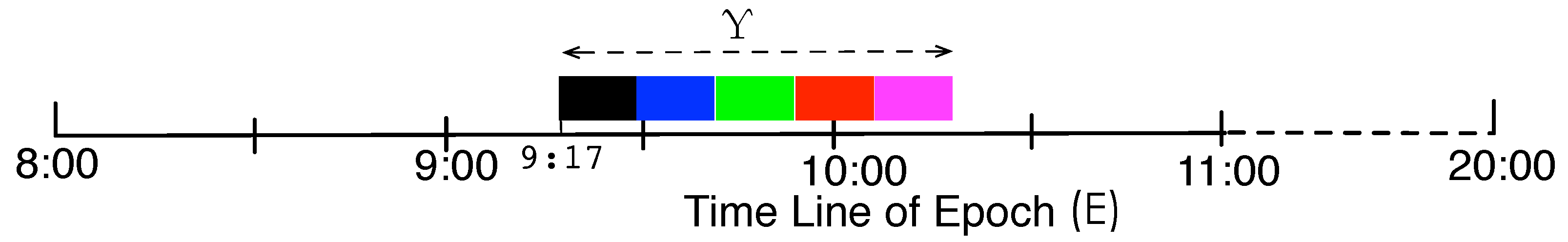
Figure 2 illustrates an example of data gathering schedule within an epoch, where the length of a round of data gathering is 60 min (Υ) and the length of epoch is 12 h (8:00–20:00). According to the optimized schedule,
would begin the data gathering trip at 9:17, and there are 5 nodes at the set of to-be-visited proxy nodes, where each time slot of visiting is denoted by the colored rectangle. The overall goal of ADG is to gather the maximal amount of data from nodes during the constrained time period at the right place, and to avoid redundant or long hops of message transmissions.
Table 1 lists the Notations and their definitions in the paper. In the following subsections, we present the detailed description of main phases of the algorithm.
Figure 2.
An example of data gathering schedule within an epoch.
Figure 2.
An example of data gathering schedule within an epoch.
4.2. Meta-Data Extraction
In ADG nodes record and extract the network meta-data to facilitate data gathering. Each node periodically records its location and encountered nodes, based on which the meta-data about the node activity and contacts could be derived.
4.2.1. Activity Meta-Data
Suppose within a time interval
the locations in the trajectory of node
is
, where
corresponds to the recorded location of node at time
. Then the
activity range of node
is defined as follows:
where
denotes the Euclidean distance of point
a and
b, and
is the geometric center of the recorded points. The centroid
is defined as:
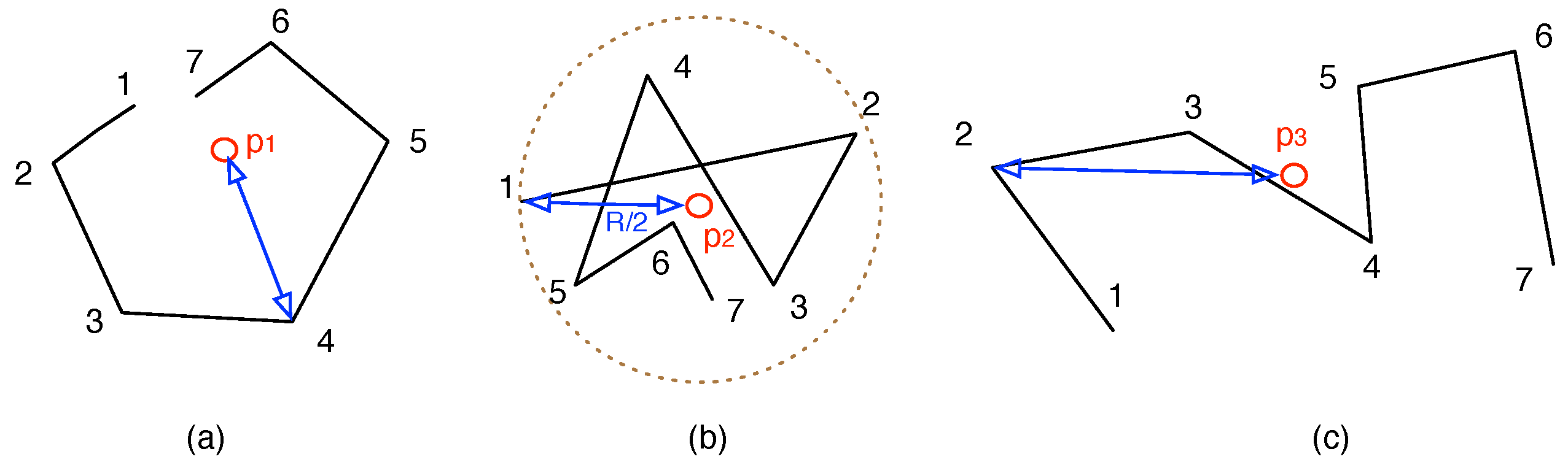
Figure 3.
Examples of node trajectories and their activity ranges: (a) moving trajectories of node ; (b) moving trajectories of node ; (c) moving trajectories of node .
Figure 3.
Examples of node trajectories and their activity ranges: (a) moving trajectories of node ; (b) moving trajectories of node ; (c) moving trajectories of node .
Based on the activity range, ADG then calculates the time duration and the central point when a node stays stationary or only roams within a small area. We abstract these as the
stationary stay (
), which is defined as
.
is the
stationary duration,
is the central location within the duration.
follows the following conditions:
where
τ is the minimal time length of stationary duration,
E is the time range within an epoch, e.g., [8:00, 20:00],
R is the communication range of the node. Here the activity range
is less than half of the communication range
R, so any two nodes, if they are both within the circular area centered at
, could communicate with each other and makes the message exchange.
Figure 3 illustrates examples of the trajectories and their average ranges. The lines are the moving trajectories of the nodes, the numbers denote the timestamps at that position,
is the centroid and the line segments in blue color is the activity range
. We could see that node
has smallest
, yet node
has the largest
. Also, if
, then the stationary duration for node
is
, and any node within circle
could communicate with
during the time period.
Figure 4.
Mapping the maximal stationary durations () into set of key stationary durations () with threshold .
Figure 4.
Mapping the maximal stationary durations () into set of key stationary durations () with threshold .
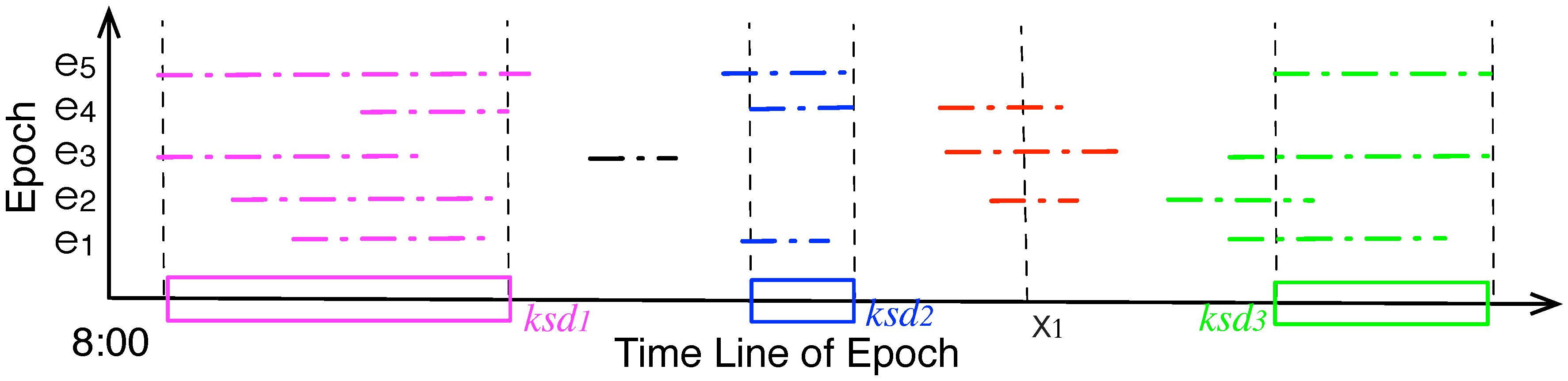
A node usually has more than one stationary stays in an epoch, and it records multiple stationary stays after several epochs.
Figure 4 illustrates an example of stationary durations during an observing window of 5 epochs. The x-axis is the line of epoch, e.g., 8:00 to 20:00, the y-axis denotes
of the epochs. The colored line segments are the static durations (
) at different epochs, and
’s from multiple epochs could be aggregated into the key static durations (
), which are denoted by the colored rectangles. Given an observing window
W, the expected probability that a point, e.g.,
x, is within a stationary duration is estimated as:
where
f is a weighting function,
is a function signifying 1 or 0. When time
x is within a
in epoch
,
=1, and the weight
equals
; otherwise,
=0, and the weight
is 0. We assume later
has larger impact on the weight. Although various weight degrading functions could be used, here we use a simple one: the weight is divided by
, which means the weight of a
is twice of that of the previous one. As illustrated at
Figure 4,
lies within a stationary duration at the 2nd, 3rd and 4th epochs, the estimated probability of
is:
=
=
= 0.4375.
ADG then aggregates and maps the
stationary durations (
) into a set of
key stationary duration (
). All points in the
has a estimated probability greater than a threshold parameter
θ, and it means the node would stay stationary or only roams within a small area during the time interval
with probability higher than
θ. A
should meet the following conditions:
Condition 2 means
is the maximal superset of the range, and it does not exist another key static duration that contains the
.
Figure 4 also illustrates the set of
with
(is also the default value in simulation), and readers could refer to
Appendix A for the detailed algorithm that extracts a nodes’s the
.
A stationary stay is denoted as , where is the stationary duration and is the central point. Correspondingly, stationary stays are mapped into a key stationary stay (), and a key stationary stay is denoted as . Here Ω denotes the possible locations and their weights the node might be in during the key stationary duration .
A node might have multiple key stationary stays. The set of key stationary stays of node
is denoted as
, then the
accumulated weight of stationary stay of node
is denoted as
, which is a key factor for the proxy node selection:
where
denotes the length of key stationary duration in
,
is the number of elements in the set. From the equation, we could see that
goes up when the
have longer accumulated time length and are distributed to more separated segments on the time line of an epoch.
4.2.2. Contact Meta-Data
Nodes also record their encountered nodes as contact log (). Tuple in is in the form of , where is the of encountered node, and denote the beginning and the end of the contact respectively, and the contact duration should be greater than a predefined threshold. Based on the contact logs, the number of distinct contacts of , denoted as , could be calculated. η is a key parameter for proxy node selection. The larger η is, the more active the node would be, and the more suitable for the node to be a proxy node.
Also, ADG adopts an opportunistic strategy when forwarding messages in MON. A node, e.g.,
, could calculate the encounter probability with any other node given an observing time window
W:
where
g is a user-defined weighting function,
is a function signifying 1 or 0. When
encounters
at
epoch,
=1, and the weight is
; otherwise, when they do not encounter each other,
=0, and the weight is 0. The calculation is similar with that in Equation (
4), and we assume later contacts has greater impact on the weight. For example, when |W|=4, if node
encounters
at the 2nd and 4th epoch, the encounter probability
=
= 0.625.
4.3. Proxy Node Selection
At initial epochs, nodes exchange meta-data with other nodes through opportunistic communications, e.g., epidemic routing [
31]. When
moves within the field, e.g., following the random waypoint mode, the neighboring nodes would send their sensed data and meta-data to the collector. After some time,
would have accumulated enough meta-data for the selection of proxy nodes.
The proxy selection is based on the
of a node, which is composed of two parts: the
accumulated weight of stationary stay and the
number of distinct encounters :
where
is the balance factor,
is defined at Equation (
6),
is the distinct number of nodes that contact with node
.
and
are the maximal values of corresponding parameters
has ever known. They could be extracted by
through initial rounds of data gathering and meta-data exchanging. Parameter
and
are then broadcasted to the sensing field, and every node would use these parameters to calculate its weight. If
is greater than a predefined threshold
, or a node is a proxy node in previous epoch yet does not upload its data to
, then
would promote itself as the proxy node at current epoch. Also, the number of proxy nodes could be controlled by the parameter settings. Proxy nodes act as the intermediate data storage as other nodes would forward their sensed data to them; then the mobile collector would come and pick up the data from the proxy nodes.
It is worth to be noted that given the , and , a node could determine whether it would act as a proxy node or not. If a node changes its state of role, e.g., to be newly promoted as a proxy node or turn back as a ordinary node, it would advertise itself by broadcasting a state-change message. In this way, other nodes and will be informed on that change. Also, although nodes are classified into ordinary nodes and proxy nodes, the network is not partitioned into clusters of subregions or subnetworks, e.g., a node is attached to some cluster and it only route its data to the cluster head. Instead, within the network all nodes are mobile, and they adopt an opportunistic way for message transmissions. When two nodes are in contact, they would establish a temporary communication link for message exchange. Ordinary nodes would forward their data to the proxy nodes whoever they encounter.
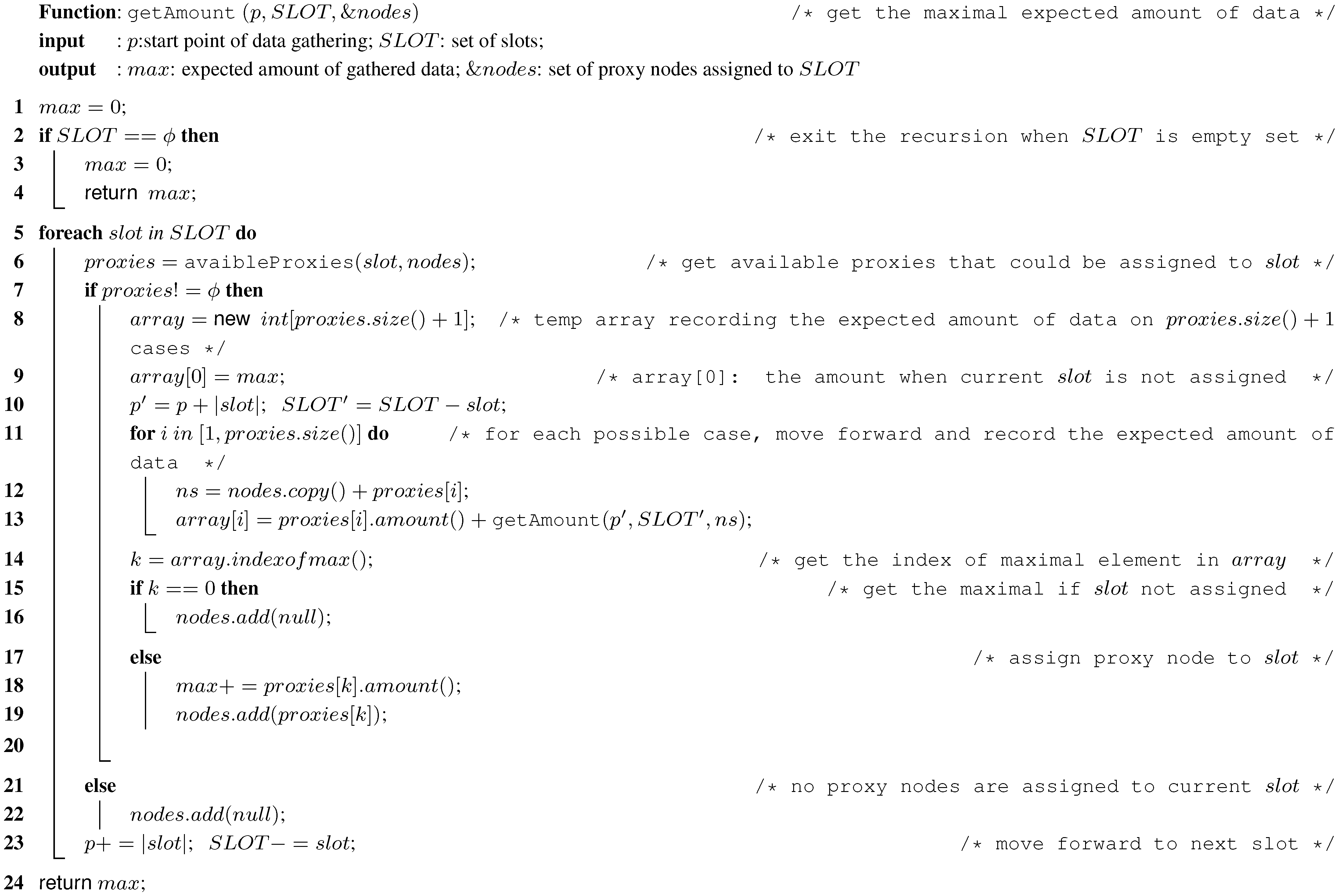
4.4. Visiting Order Scheduling
Once proxy nodes gather the sensed data from their neighboring nodes, these data should be collected by the mobile collector when they are in contact. Usually there are more than one proxy nodes, and has to arrange its visiting order and time slots so that it could gather the maximal amount of data within the limited period. The scheduling could also be viewed as the Proxy node Time Slot Allocation (PTSA) problem.
PTSA Problem: Given a set of proxy nodes V, find a set of proxy nodes and their visiting schedule Ψ during the data gathering period Υ, such that the expected amount of gathered data χ is maximized and the schedule Ψ is .
Firstly, the expected amount of gathered data by visiting the set of proxy nodes
is estimated as:
where
is the expected amount of data stored at a proxy node,
is the number of distinct contacts of
,
denotes the amount of data a node might have in data gathering round
r.
Secondly, when a scheduler is
, the collector would visit each of the nodes one by one within the data gathering period
, and would not conflict with each other. Formally, a schedule
is said to be
if it follows the following condition:
where
denotes visiting
during the time range
,
denotes one of the key stationary duration of
, and
is minimal data gathering duration of a slot. Each slot is assigned to a proxy node for
’s visiting, and they would not overlap with each other. Because the mobile collector could move fast, here we assume the time duration moving from one proxy node to the next is negligible compared with the period of data gathering round. So the collector
is only constrained by the duration of data gathering, which is denoted by Υ.
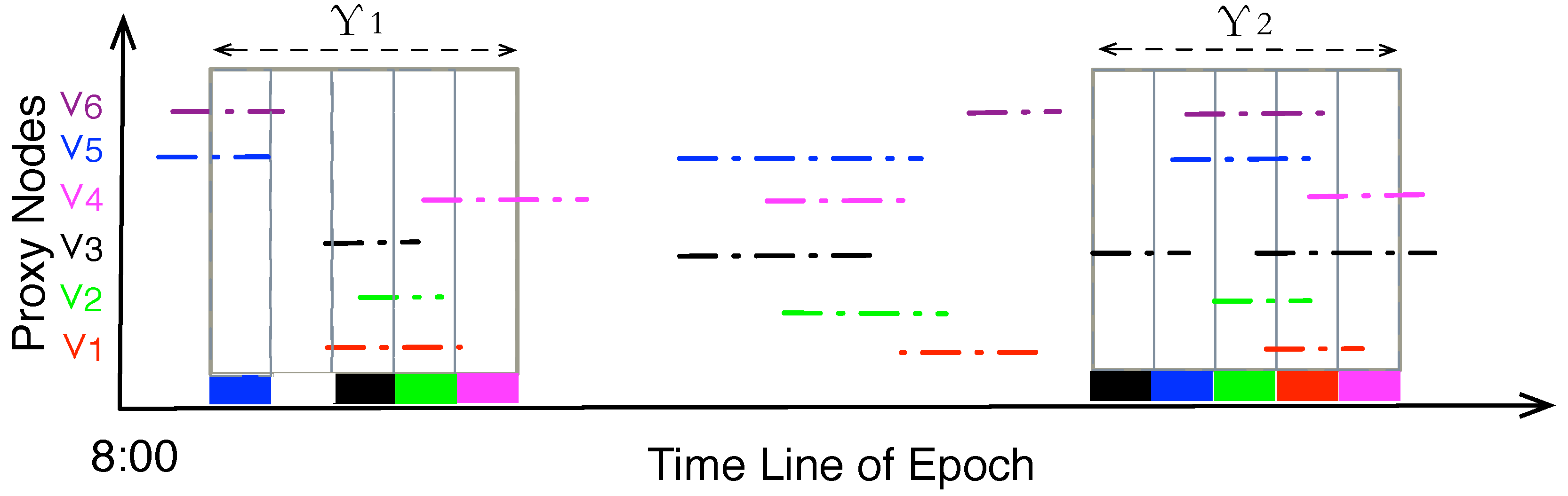
Figure 5.
Mapping the Proxy node Time Slot Allocation () problem into the problem of maximal coverage of line segment.
Figure 5.
Mapping the Proxy node Time Slot Allocation () problem into the problem of maximal coverage of line segment.
The PTSA problem is a variant of the famous “Knapsack problem” [
20]: given a set of proxy nodes, each with an amount of data to be gathered, determine the set of proxy nodes to include in the data gathering period so that the total amount of data is as large as possible, under the constraints that the visiting of proxy nodes should be continuous and the
key stationary stays should not overlap each other in the time dimension. This problem is also defined as the
maximal coverage of line segments, where the covering line is the data gathering duration. In
Figure 5, the x-axis is the line of epoch, e.g., 8:00 to 20:00, the y-axis denotes id of the proxy nodes. The colored line segments are the key static durations (
) of different proxy nodes. The key stationary durations (
) are projected on the time line of epochs (x-axis ), and they overlap with each other. ADG then calculates a period of data gathering round with length Υ, and assigns each of its slots to a proxy node, so that the total
of the slots is maximized. Here the
of a time slot is the expected amount of data that could be gathered by the
during that slot. When a proxy node
v is assigned to a time slot
s,
is supposed to encounter
v and gather its stored data, so the weight of
s is the total amount of data stored at
v. From the figure, we could see that
is preferred compared with
because it covers more slots, and hence might get more amount of data from the proxy nodes. Note that the duration Υ could only cover a slot exactly once because within an exact time slot
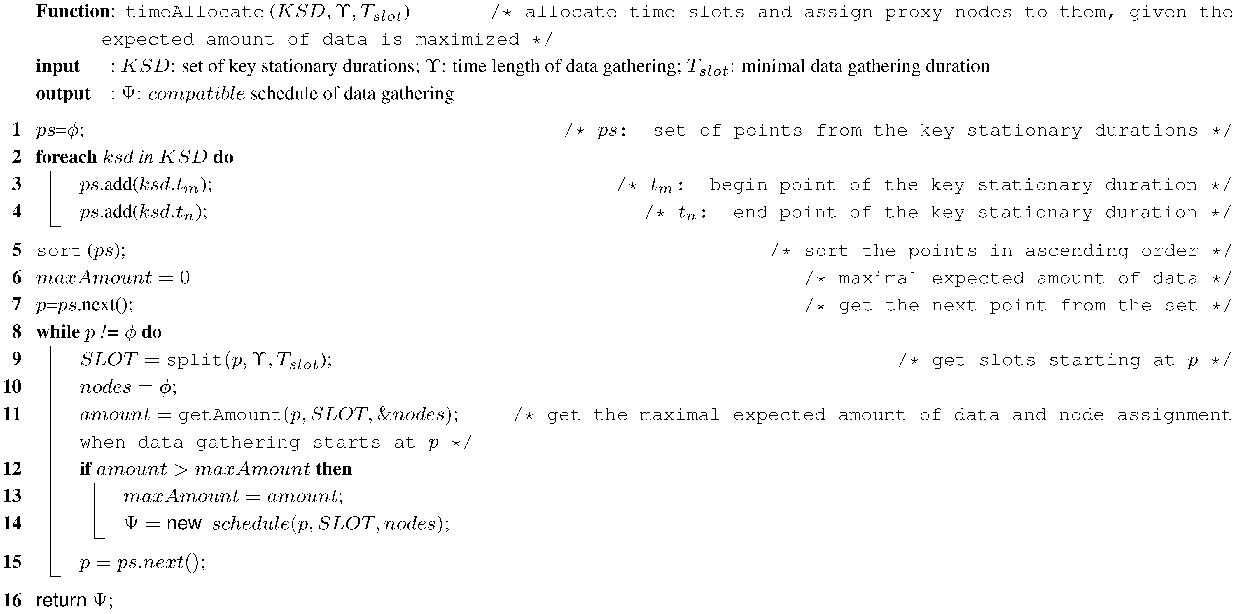
could only visit one proxy node, and hence could prune large searching space. Readers could refer to
Appendix B for the detailed algorithms that solves the PTSA problem.
It is possible that some proxy nodes, e.g.,
in
Figure 5, might not be visited by
within a gathering round. In ADG, the unvisited proxy node would double its weight
at the next round of data gathering, meaning more data is stored at the node. So at the next epoch the unvisited proxy node would be added to the
to-be-visited set of nodes according to the algorithm, and the data could be picked up by the data collector.
4.5. Data Gathering from Proxy Nodes
When a new data gathering round begins, would visit the proxy nodes one by one according to schedule Ψ. When they are in contact, the sensing data that have been routed and stored at the proxy nodes are gathered by . Proxy nodes has high probability to be stationary and hence be able to make a stable connection for data transfer. Yet still has to figure out the location of the proxy node in order to visit a proxy node during its key stationary stay () according to the schedule.
For a proxy node
v, suppose the key stationary stay
is mapped from
m stationary stays from
m epochs, where each stationary stay is composed of a stationary duration
and the central point
; then the set of
m central points are aggregated according to their locations. A set of central points, e.g.,
, could be aggregated into a new point if they satisfy the following conditions:
where
R is the radius of communication range. Points in
Q could then represented by a new point:
, which is defined at Equation (
3). Similar with the expected probability of a point defined at Equation (
4), the
encounter probability of
is then defined as:
where
is the index of epoch from which the central point
is extracted. The data gathering point for proxy node
v is then set to be the point who has the largest encounter probability, denote as
.
then just moves to point
and prepares for encountering the proxy node and gathers the data.
Although the node movement is assumed to roughly follow some kind of pattern within the network, and nodes would stay at some area during the key stationary duration with high probability, it is also possible that a proxy node deviates from the expected location and moves to other area. At this case the proxy node would periodically broadcast its locations to its neighboring nodes so that is able to get the proxy node’s exact locations from neighboring nodes, and move to the new location to pick up the data during the data gathering time slot. also collects data from ordinary nodes when they are in the communication range, and gathers the network meta-data for proxy nodes selection and time slot allocation in the next epoch.
5. Experimental Section
5.1. Environment Setup
We implement ADG in C# and compare it with other data gathering schemes. As nodes are mobile, we assume relatively sparse deployment of nodes for the wireless sensor network: there are 36 nodes within a rectanglar area, and the network is divided into 8*8 grids. The community model described in [
32] is adapted to simulate the movement of nodes, where each grid is a community and each community has an interest index
. If the index is greater than a threshold, the community is called a
Hot Community, and the set of hot communities in the network is denoted as
C. At the beginning of the simulation, each node is tagged as
ordinary node, and each ordinary node is assigned an
, e.g.,
, and an grid as its
home community. Each node starts its movement from its home community, moves along its path, and then goes back to the home community. Each node moves according to a set of paths, and each path is composed of several communities, including the hot communities. A node stops and moves within community
for a period with probability of
; and chooses to move to the next community along the path with probability
, where
is the predefined value,
is the interest index of the target community.
represents the probability that a node would stop because of the distraction within the community that it currently visits. A node has several predefined paths, and the path to move along is randomly chosen from them. An ordinary node may promote itself as a proxy node and change its tag to
proxy node according to
Section 4.3, yet this has no impact the node movements. The
is not active until a data gathering round is fired. It moves to the predicted location of proxy nodes one by one according to the optimized schedule, stop at each location for a period of time expecting to receive data from the proxy nodes.
Table 2 summarizes the default values of network model and parameters in the simulation.
The simulation runs periodically. It consists of 30 epochs, where each epoch has a period of 14,400 simulation seconds (s), and the length of data a gathering round (Υ) is 1800 s. For the sensed data, every node adopts a Poisson process to trigger an event for data generation, where the interval between two sequential events follows the Poisson distribution with parameter λ = 600 s. The size of date generated by an event is 64 K, so the expected amount of total sensing data generated by a network of 36 nodes is 54 M (36*64 K*14400/600) per epoch. The bandwidth of link that uploads data from ordinary nodes to is 64 KBps. We assume ideal links when two nodes meet and establish a connection.
ADG is a data gathering scheme that adopts speedy mobile elements at opportunistic mobile sensor networks under limited data gathering period. It is worth noted that “opportunistic forwarding” and “limited data gathering period” are the two main characteristics of the proposed ADG scheme compared with other data gathering schemes. Ordinary nodes would move to other places, and tracks could not be predefined or calculated for the data collector. So the track-base or roaming-based data gathering schemes [
3,
4,
6] could not be directly adopted for the data gathering scenarios of opportunistic mobile sensor networks. For fair and extensive comparison of the proposed algorithm, we implemented other four data gathering schemes that adopt opportunistic forwarding or proxy based strategies:
(1) Epidemic [
31]:
moves according to the way-point mobility model, yet nodes take advantage of all chances of communications, data are exchanged among any nodes if possible and finally gathered by the
;
(2) PROPHET [
32]:
moves as the same pattern in Epidemic, yet data are exchanged according to the data forwarding probability based on the movement history;
(3) PDA [
13]: a node contact graph is created to compute the data gathering location where
could contact with more nodes during some time period;
is then programmed to move to the gathering point to gather the data;
(4) PROXY: nodes with more contacts are promoted as proxy nodes. Proxy nodes broadcast their location information to notify neighboring nodes for opportunistic data collection, and
would visit the proxy nodes according to a scheduled trajectory. The trajectory planning is similar to reference [
25] based on the solution of the Traveling Salesman Problem.
Table 2.
Default parameters of the simulations.
Table 2.
Default parameters of the simulations.
| Parameter | Value | Description |
|---|
| N | 36 | number of nodes |
| 800*800 m | area of the sensing field |
| 10*10 | grid partition of the field |
| | initial and total number of epochs |
| s | length of an epoch |
| 8 | number of epochs in observing window |
| Υ | 1800 s | data gathering round for |
| 9 | number of slots (200 s/slot) |
| , | [2, 4], [10, 20] m/s | node and ’ range of speed |
| | nodes’ basic probability that stops at a grid |
| | nodes’ stop duration at a grid |
| C | 24,31,36,45,
50,54,67,76,83 | set of hot communities |
| | rang of number of hot communities for a path |
| 2 | maximal number of paths a node has |
| | range of number of grids in a path |
| α | | balance factor at Equation (8) |
| | threshold for proxy node selection |
| 128 M | size of cache for a node |
| 1 K | size of a packet |
| R | 30 m | nodes’ communication range |
| B | 64 KBps | bandwidth for communication |
| 64 K | size of date generated by an event |
| λ | 600 s | Poisson parameter for events |
Epidemic and PROPHET are two classic routing protocols for opportunistic data forwarding; PDA is based on the opportunistic forwarding and contact graph; PROXY is close to ADG in that ordinary nodes route their data to the proxy nodes using opportunistic forwarding schemes, e.g., the Spray and Wait scheme [
33]. The differences lies in that in PROXY the selection of proxy nodes does not consider the mode of node movements (e.g., stationary stay, contact duration), and proxy nodes have to proactively broadcast their locations to notify
when
schedules its path to gather data from the proxy nodes.
5.2. Overall Performance
In
Table 3, row 1 lists the average number of messages of meta-data exchange, row 2 lists the number of messages that upload data to
, row 3 lists the number of total messages per epoch, row 4 lists the
data coverage, and row 5 lists the
efficiency of the algorithms. The results presented at each cell is the average of 6 rounds of simulations, given the default parameters such as number of nodes, the data gathering period, and etc. At the simulation all the nodes are mobile, and they take advantage of the opportunistic communication chances for the data gathering. So each node is randomly assigned to a home community at each simulation and has its own paths, where the paths are different from one simulation to another.
For the overhead of message transmissions, all schemes except Epidemic incurs the cost of meta-data exchange and gathering. The number of messages for meta-data exchange is low, and it accounts for less than 15% of the overall message transmissions. Epidemic has no overhead of meta data exchange, yet it has the largest message transmission, as high as about 4.52E+5. This is because messages are exchanged among all the ordinary nodes; while at other schemes messages are selectively forwarded. At PROPHET, messages are forwarded to nodes who have larger probability to meet the , and at other schemes messages are only forwarded to the proxy nodes, saving lots of in-network message transmissions. So the overall data transmissions of PDA, PROXY and ADG are relatively small, which is more than 40% less than that of Epidemic. The amount of data upload messages is directly related to the data coverage. ADG has the largest data coverage, so the number of messages that upload the data to is the largest. receives about 3.99E+4 messages of sensed data from other nodes.
Table 3.
Comparison of the overall performances.
Table 3.
Comparison of the overall performances.
| Id | Metric | Epidemic | PROPHET | PDA | PROXY | ADG |
|---|
| 1 | Meta Exchange | 0 | 1.83E+4 | 2.89E+4 | 2.94E+4 | 2.62E+4 |
| 2 | Data Upload | 5.77E+3 | 4.80E+3 | 1.97E+4 | 2.85E+4 | 3.99E+4 |
| 3 | Total Mssage | 4.52E+5 | 3.39E+5 | 1.85E+5 | 2.16E+5 | 1.78E+5 |
| 4 | Data Coverage | 10.43% | 8.45% | 35.64% | 51.50% | 72.12% |
| 5 | Efficiency | 4.88% | 5.02% | 28.36% | 32.62% | 43.21% |
Data coverage is defined as the amount of collected data divided by that of the total sensed data. From the table we could see that ADG has the largest data coverage, it gathers about 72.12% of the sensed data; while PROXY and PDA gathers 51.5% and 35.64% on average. The data coverage at ADG is about 6–8 times of those in Epidemic and PROPHET. at Epidemic and PROPHET could only collect data from whoever it encounters. Most of the data are not gathered because the data gathering period is relatively short, e.g., 1800 s. Instead, PDA, PROXY and ADG selectively compute the data gathering points; they guarantee a possible sojourn location that more data could be picked up by the . For PDA, the data gathering location is a place where more nodes get together; while in PROXY and ADG the data gathering locations are a set of proxy nodes, which are visited by for data gathering. However, due to the movement of proxy nodes, at the PROXY scheme might lose the track of the proxy nodes. At this case, gathering data from proxy nodes might not be feasible. At the ADG scheme, the sojourn location and time for the proxy nodes are carefully calculated, so would encounter the proxy nodes and picks up the data with high probability, leading to higher data coverage.
Metric efficiency is defined as the number of messages divided by the number of total messages. Messages are defined as if they are related with successfully uploaded data. They are the messages that are sent from the source node, forwarded among intermediate nodes, and successfully uploaded to . Efficiency is as high as 43.21% in ADG, while they are 4.88%, 5.02%, 28.36%, and 32.26% for Epidemic, PROPHET, PDA and PROXY respectively. This means more than 90 percent of the message transmissions at Epidemic and PROPHET do not lead to final successful data upload to ; at other schemes the data gathering locations are carefully calculated, and there are proxy nodes for intermediate data storage, so more sensed data could be uploaded to and hence have higher efficiency.
5.3. Impact Factors Analysis
From the overall performance analysis we could see that ADG has great improvement compared with other schemes on the data coverage and overhead of message transmissions. ADG is specially suitable for data gathering at mobile sensor networks under limited data gathering period. The advantage lies in the careful selection of proxy nodes and their best stationary period so that there exists stable communication link for to pick up data from these nodes. In this subsection, we vary the basic network parameters to study their impacts on the performances of data gathering schemes.
5.3.1. Network Density
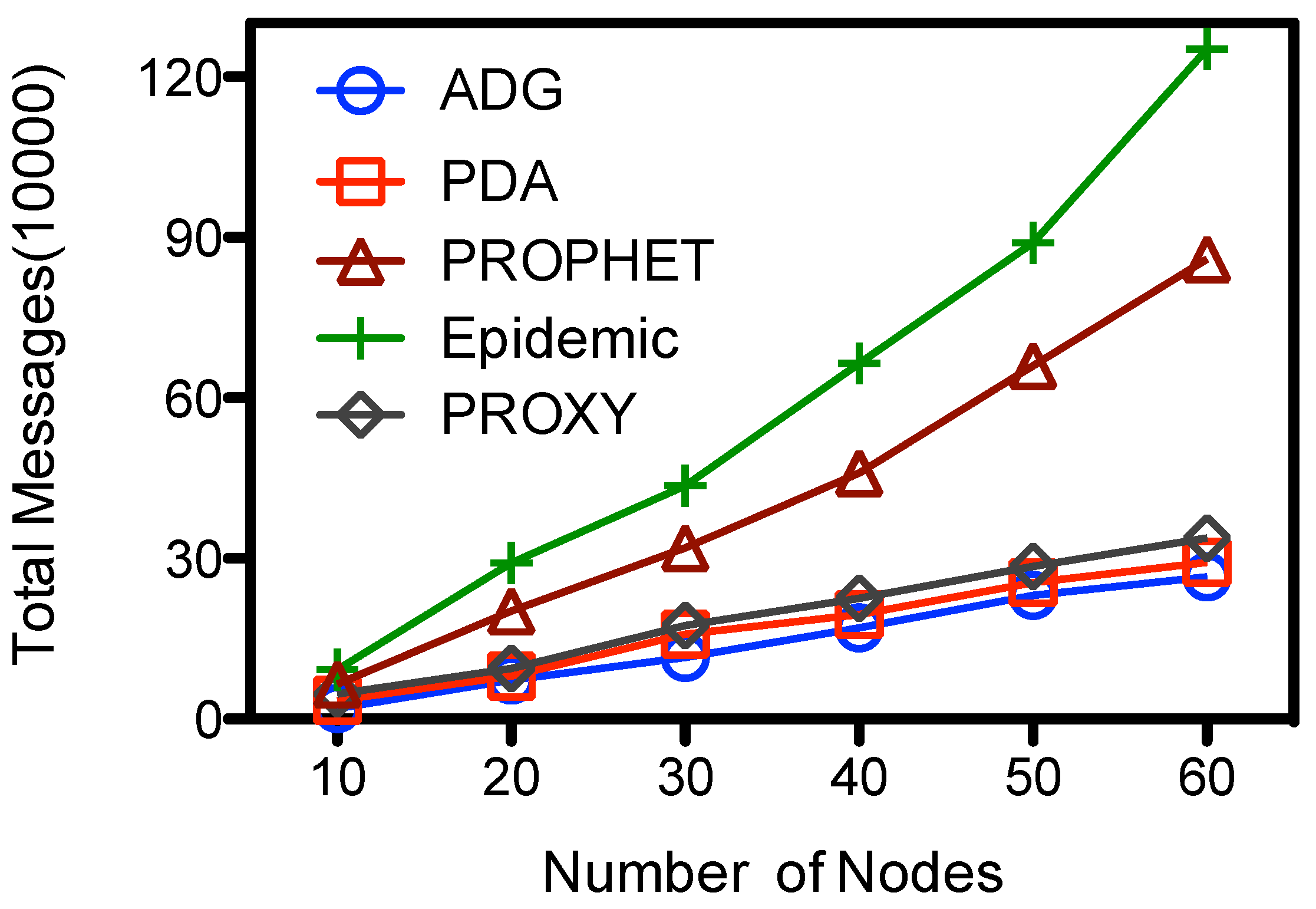
From
Figure 6 we could see that the number of message transmissions of all schemes goes up with the number of nodes. The Epidemic has the largest message transmissions, the number increases from 6.54E+4 to about 1.25E+6. Messages are exchanged among any two encountered nodes at Epidemic, while in other schemes the messages are selectively forwarded among the nodes. At the PDA, PROXY and ADG schemes messages are first selectively forwarded towards the proxy nodes, and then picked up by the
. The former dominates the total cost of message transmissions, so the number of total message transmissions are very close. They have the lowest total message transmissions of the compared schemes, and the number is less than 25% of that in Epidemic when there are 60 nodes at the network. The performance of PROPHET lies in the middle, the number of transmissions is about 64%–70% of that at Epidemic at our simulation setting. For the proposed ADG scheme, ordinary nodes would sent their sensed data to the proxy nodes before the data are picked up by
. There would be fewer messages exchanges among ordinary nodes in a sparse network because nodes would have fewer encounters. When there are more nodes, e.g., 60, the message transmission would goes up to about 2.65*E+5 at ADG, which is about 13 times of that when there are 10 node.
Figure 6.
Number of nodes vs. total message transmissions.
Figure 6.
Number of nodes vs. total message transmissions.
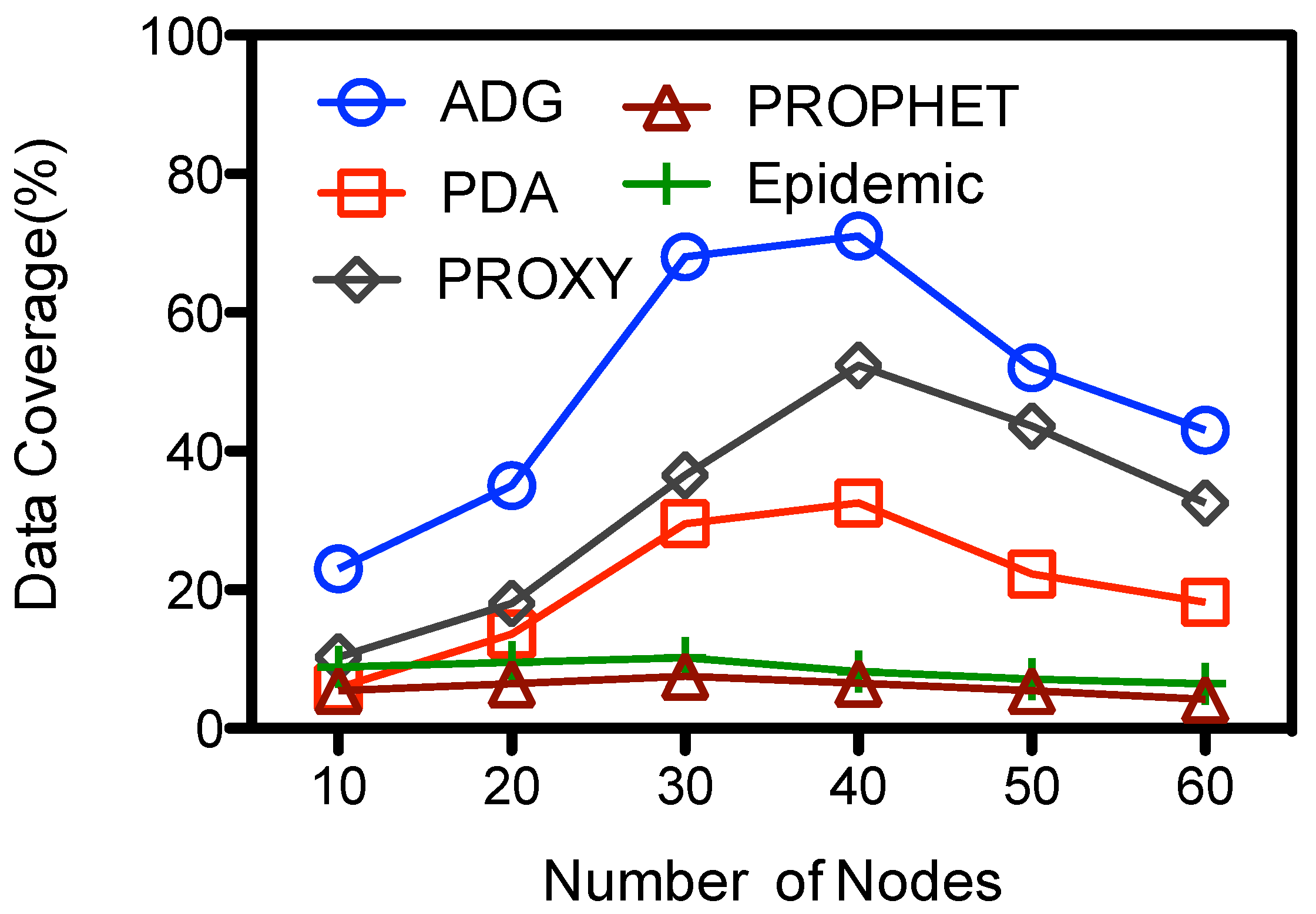
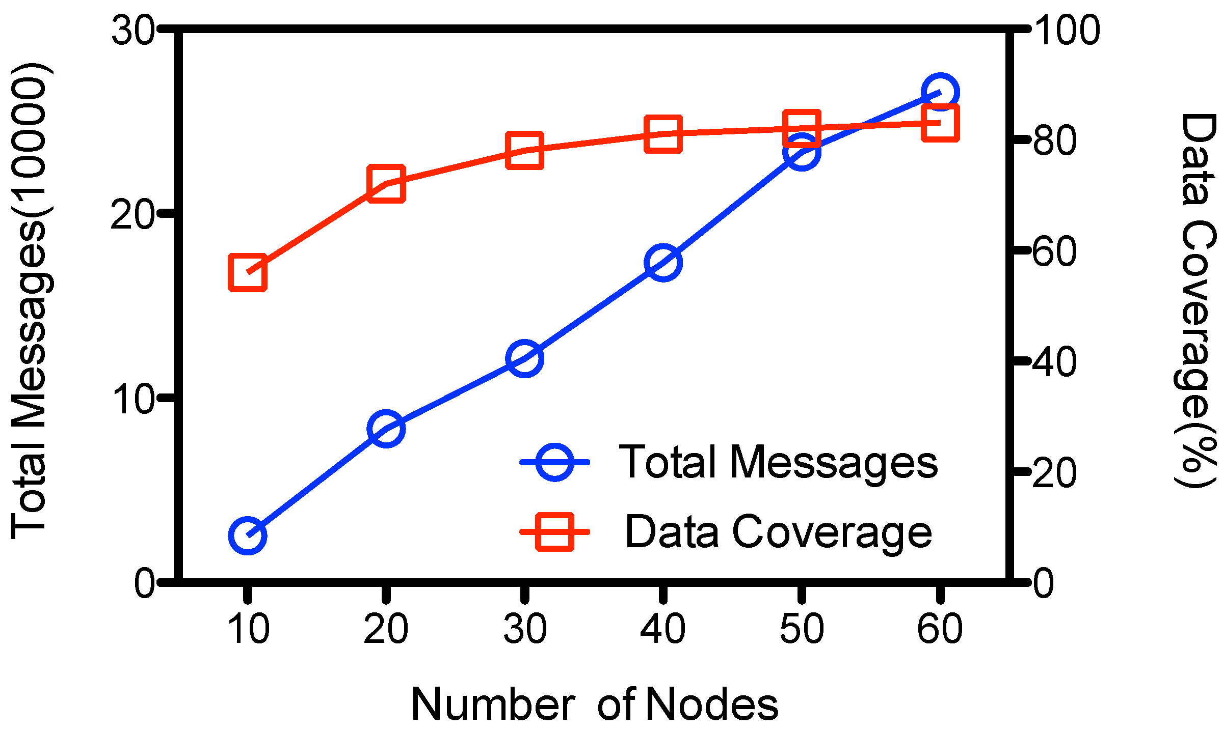
Figure 7 shows the impact of network density to the data coverage. Epidemic and PROPHET has the smallest data gathering rate. Their data coverage decreases a little bit with the number of nodes, and the overall data coverage is less than 10.2%. This is mainly because of the limited data gathering period, which is about 12.5% of the total epoch. For other schemes their data coverage firstly goes up with the number of nodes, and reaches as high as about 72%, 52% and 32.5% for ADG, PDA, and PROXY respectively when 40 nodes are deployed. Proxy nodes would have more contact opportunities and receive data from ordinary nodes when there are more nodes within the network at these schemes. Yet ADG has higher data coverage because
could collect the data from a set of proxy nodes while
has only one data gathering location at PDA. Although there are multiple proxy nodes at the PROXY scheme,
might lose the track of the proxy nodes as they keeps moving within the data gathering period. So the data at some proxy nodes could not be upload to the
, which harms the data coverage. For the ADG scheme, when there are more nodes in the network, e.g., more than 40 nodes, there would be too many proxy nodes that act as intermediate storage to be visited by the
. However, because the data gathering period is limited due to energy concern,
is not able to collect all the data from the proxy nodes at one epoch, which decreases the data coverage. The data coverage is about 43% when there are 60 nodes and with one data collector.
However, it is easy to extend ADG using multiple collectors, or having multiple data gathering rounds at each epoch to handle the scalability problem of the data gathering.
Figure 8 shows the performance results that use two data collectors. The amount of total transmissions is roughly the same with that at
Figure 6, but the data coverage increases with the number of nodes due to the increased chance of contacts and meta-data exchanges within the network. It gathers as high as 82 percent of the sensed data when there are 60 nodes in the network. Generally, the number of collectors and the number of data gathering rounds could be tuned according to the network density and the data generating rate of the network.
Figure 7.
Number of nodes vs. data coverage.
Figure 7.
Number of nodes vs. data coverage.
Figure 8.
Performance of ADG with 2 .
Figure 8.
Performance of ADG with 2 .
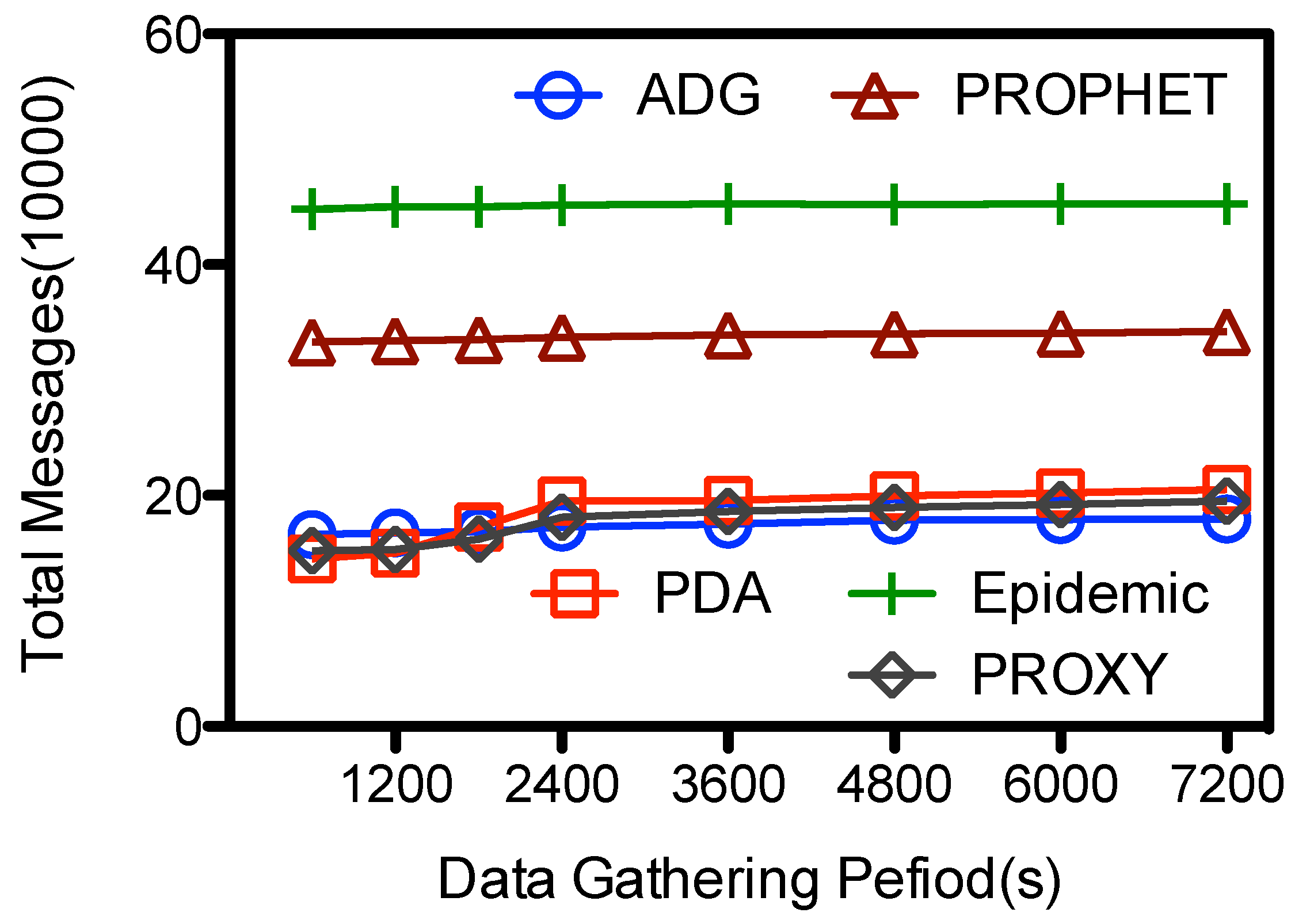
5.3.2. Data Gathering Period
Another impact factor is the length of data gathering period Υ, which is the period when
are within the network. From
Figure 9 we could see that the lines are relatively flat, showing that Υ has small impact on the number of total message transmissions. Larger Υ denotes larger contact chances between the mobile collector and in-network nodes and hence more message transmissions between them. The number of message transmissions are expected to goes up with Υ. When Υ increase from 600 to 7200 s, the number of total transmissions goes up from 1.66E+5 to 1.79E+5 for ADG, and from 1.45E+5 to 20.5E+5 for PDA. As the number of messages are mainly composed of in-network node-to-node transmissions, the impact of the increased message transmissions between
and in-network nodes is relatively small on the overall messages transmissions.
Figure 9.
Data gathering duration (Υ) vs. total message transmissions.
Figure 9.
Data gathering duration (Υ) vs. total message transmissions.
Figure 10.
Data gathering duration (Υ) vs. data coverage.
Figure 10.
Data gathering duration (Υ) vs. data coverage.
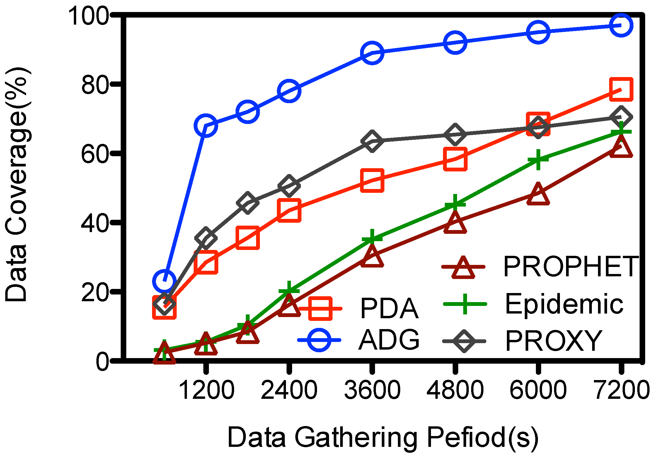
The data coverage in all the schemes goes up with Υ, as illustrated in
Figure 10. The PDA, PROPHET, Epidemic achieve their best performance at 78.5%, 66.3%, and 62.2% when the period is 7200 s; and their data coverage is less than 15% when the data gathering is limited and short, e.g., 600 s. These schemes are designed for general purpose routing and data gathering when the data gathering period is unlimited. So
might not have enough time to contact with the in-network nodes and gathers the data from them when the data gathering period is small. However, the data coverage goes up relatively sharp from16% to 40% and from 20% to 62% for the PROXY and ADG schemes respectively when Υ increase from 600 to 1200 s, and then increases to near 71% and 93% respectively when the data gathering period is about 7200 s. Both schemes use proxy nodes as the intermediate storage. However, the proxy nodes at PROXY might still be moving when the
is scheduled to collect the data from them, which makes the data transmission from some proxy nodes and
unfeasible. Instead, at the ADG scheme the proxy node is scheduled to be visited during its
key stationary duration, so message transmissions from the proxy node to the
is stable and efficient. Given a fixed time slot for each proxy node, longer data gathering period means
could visit more proxy nodes and hence gather more data from them. So when Υ is large, e.g., more than 6000 s,
would have enough time to visit each proxy node several times and pick the data up, so the data coverage goes higher. Yet in real network deployment, the data gathering period Υ is limited because the speedy
has a large energy consumption rate, and it should replenish its energy after a trip.
5.4. Impact Analysis for the ADG Scheme
Beside the basic network parameters, there are other designing factors in the proposed ADG scheme. At this subsection we study the impact of these factors, including the number of time slots, the threshold for proxy node selection, the change of node movement, and the imbalance of message transmissions.
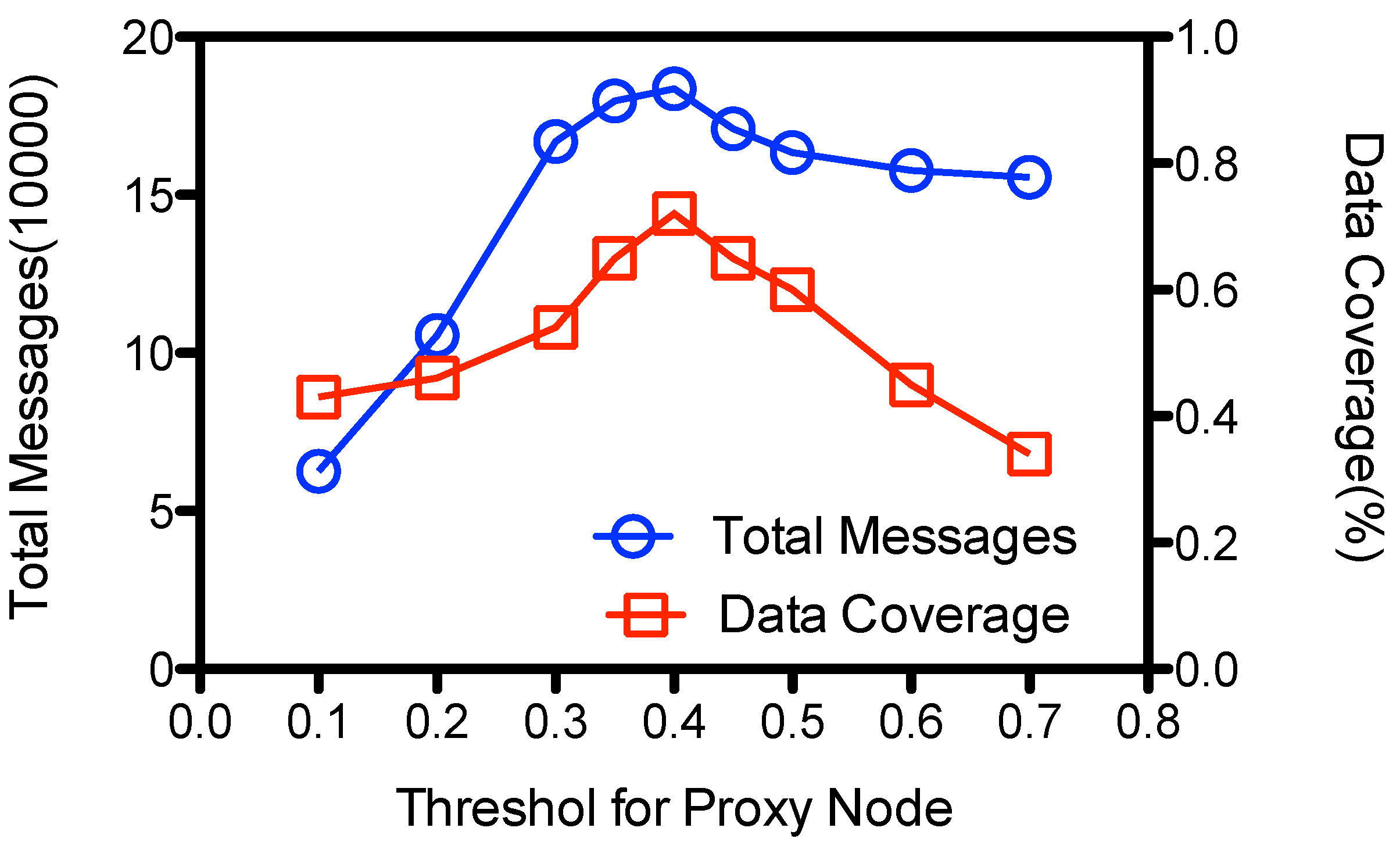
5.4.1. Threshold for Proxy Node Selection
Proxy nodes are selected according to nodes’
. According to Equation (
8), a node is promoted to be a proxy node if the
is larger than a threshold
. As showed at
Figure 11, both the number of total messages transmissions and data coverage goes up to the maximal when
is around 0.4, and then goes down as the threshold increases. When
is small, e.g., 0.1, most the nodes are promoted as proxy nodes, so they just keep the data and avoid lots of message forwarding; yet
could not visit all the proxy nodes at the epochs, leaving some proxy nodes unvisited and some data un-gathered by
, so the data coverage is low. When
is large, e.g., 0.6, fewer proxy nodes are selected, so there are fewer contact chances to upload its data to proxy nodes. This also leads to some un-gathered data at the ordinary nodes and makes the data coverage low. However, at this case the ordinary nodes would still try to forward their messages to the encountered nodes in order to be stored at the proxy nodes. So the number of total message transmissions is also high; more than 1.55E+5 messages are transmitted when
is more than 0.6. ADG achieves its best performance on data coverage at about 72% when
is within the range of [0.35, 0.5] and the number of message transmissions is about1.83E+5 at our simulation setting.
Figure 11.
Impact of threshold for proxy node selection().
Figure 11.
Impact of threshold for proxy node selection().
5.4.2. Change of Node Movement
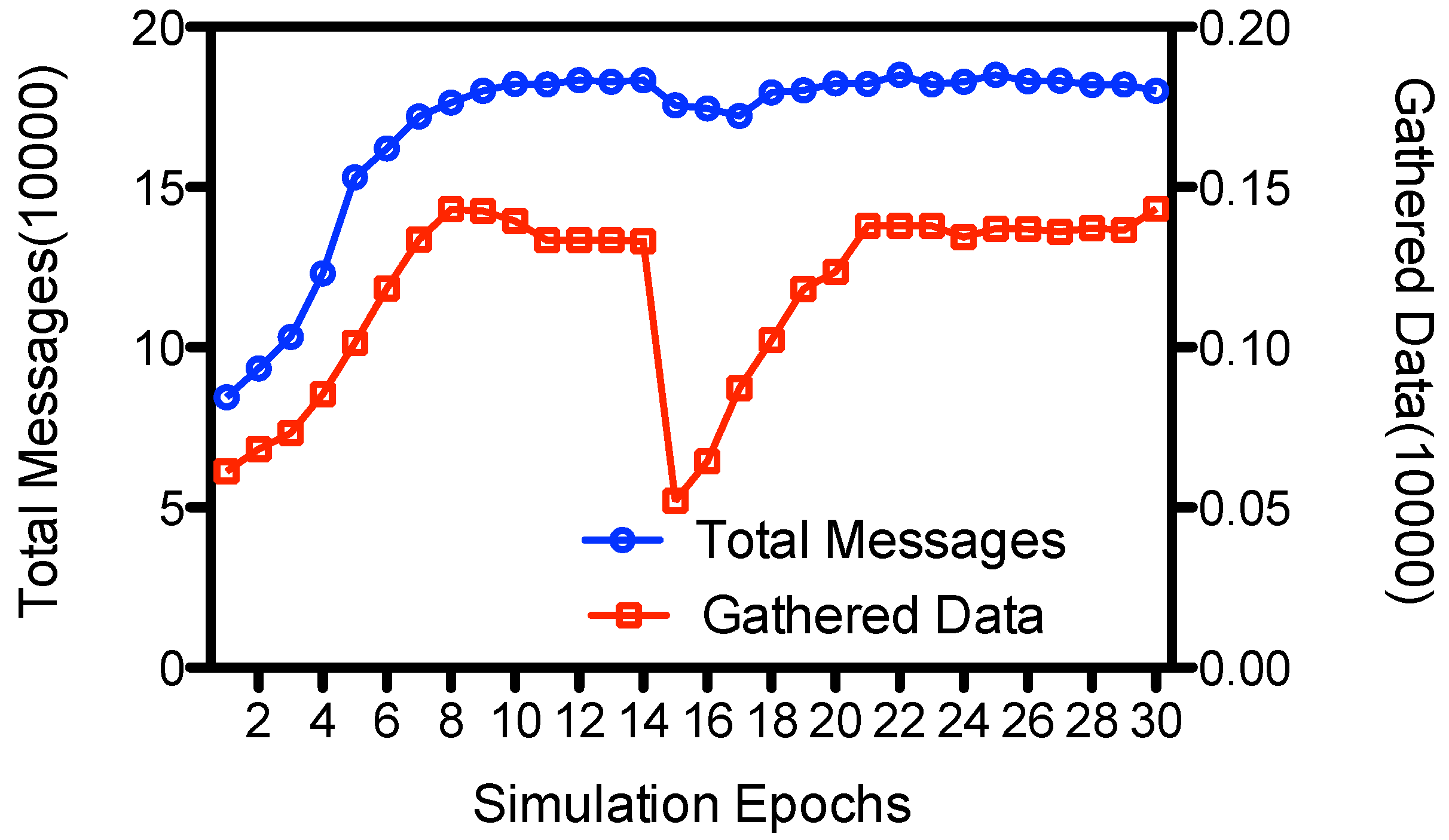
ADG gathers the meta-data and adaptively selects the proxy nodes for the data gathering. So we changed the paths of network nodes at the middle of the simulation (at the15th epoch), and studied its impact on the amount of gathered data.
Figure 12 depicts the average number of total messages and amount of gathered data at each epoch in 10 rounds of simulation. We could see that the number of gathered messages is small (less than 700 messages) at initial epochs,
i.e., from 1 to 5 epochs. This is because at initial epochs nodes exchange meta-data with other nodes through opportunistic communications. The proxy nodes has not been selected, and the only way
gathers data is that it would pick up data from its neighboring nodes when it moves within the field following a random waypoint mode. Yet after some epochs it gathers enough metadata and the proxy nodes are selected. During these epochs, nodes send their messages to proxy nodes, and
visit the proxy nodes to gather the data. So both the total messages and the gathered data would increase.
would gather about 1306 messages of sensed data at each round on average. When the node change their paths at epoch 15, we could see a sharp decline to about 521 messages on the number of gathered data. This is because
would not encounter the proxy nodes when it visits the predicted location, since the proxy nodes have changed their paths and would not appear there. However, the proxy nodes would broadcast its new locations to neighbors; and after some epochs of meta-data gathering, new proxy nodes would be selected, and
would acquire the new data gathering points of the proxy nodes. In this way, ADG adaptively updates the data gathering points and
would again gather normal amount of sensed data from the proxy nodes. The data coverage returns to about 70.8%, which is almost the same as the case when the movement of nodes do not change.
Figure 12.
Message transmissions at each epoch.
Figure 12.
Message transmissions at each epoch.
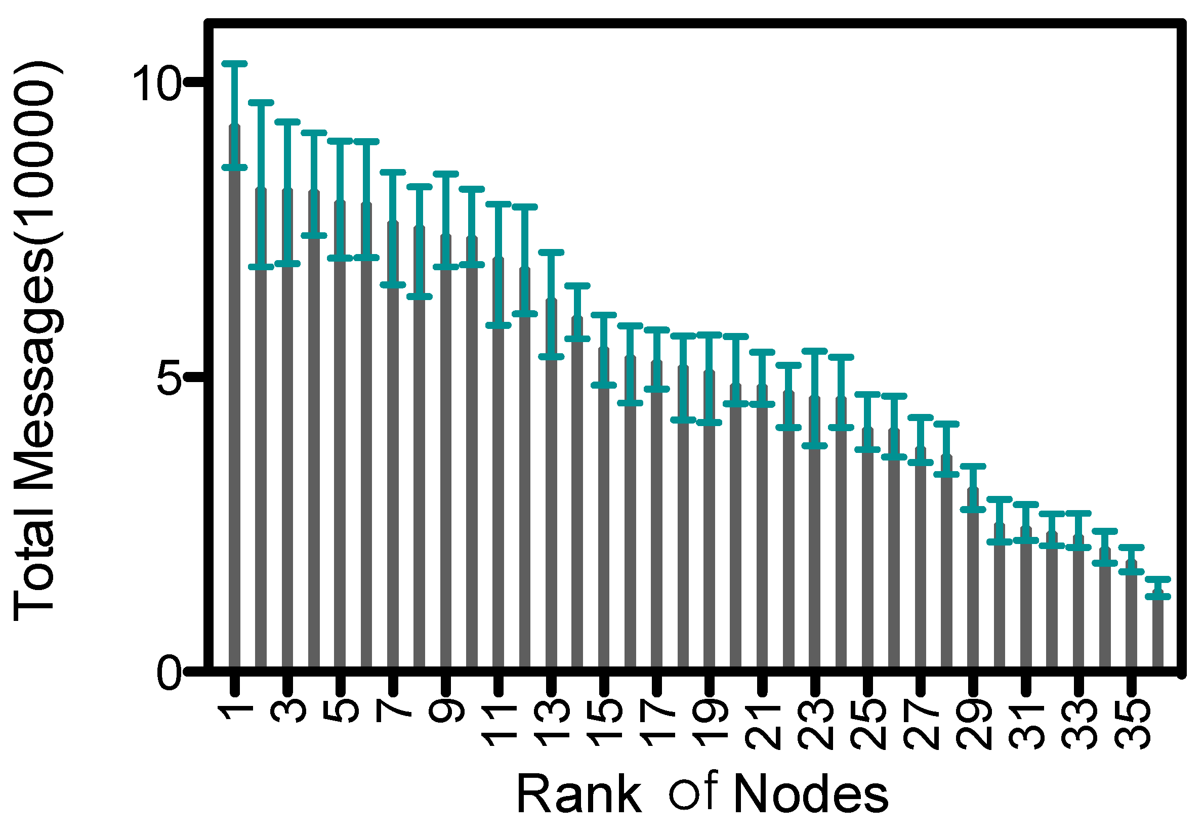
5.4.3. Imbalance of Message Transmissions
Proxy nodes receive data from ordinary nodes and upload them to the collector. So they have more message transmissions than ordinary nodes, which leads to an imbalance of energy consumption within the network.
Figure 13 shows the descending order of average number of message transmissions for nodes in 6 rounds of simulation; the upper and lower bounds are also shown. The average number of messages is about 5.26E+4 , and standard variance is 2.18E+4. In ADG proxy nodes could be recalculated and updated among epochs, which helps balance the energy consumption. However, the maximal number of message transmissions is about 6.9 times of the minimal, which would lead to early exhaustion of energy at some proxy nodes. Yet recently, the breakthrough at wireless power transfer [
34] has brought up a new possibility that
would recharge the proxy nodes at the same time when proxy nodes are uploading the data. We leave the discussion of gathering data from rechargeable nodes as our future work.
Figure 13.
Message transmissions of nodes in descending order.
Figure 13.
Message transmissions of nodes in descending order.


