HyperCube: A Small Lensless Position Sensing Device for the Tracking of Flickering Infrared LEDs

Abstract

An innovative insect-based visual sensor is designed to perform active marker tracking. Without any optics and a field-of-view of about 60°, a novel miniature visual sensor is able to locate flickering markers (LEDs) with an accuracy much greater than the one dictated by the pixel pitch. With a size of only 1 cm³ and a mass of only 0.33 g, the lensless sensor, called HyperCube, is dedicated to 3D motion tracking and fits perfectly with the drastic constraints imposed by micro-aerial vehicles. Only three photosensors are placed on each side of the cubic configuration of the sensing device, making this sensor very inexpensive and light. HyperCube provides the azimuth and elevation of infrared LEDs flickering at a high frequency (>1 kHz) with a precision of 0.5°. The minimalistic design in terms of small size, low mass and low power consumption of this visual sensor makes it suitable for many applications in the field of the cooperative flight of unmanned aerial vehicles and, more generally, robotic applications requiring active beacons. Experimental results show that HyperCube provides useful angular measurements that can be used to estimate the relative position between the sensor and the flickering infrared markers.

1. Introduction

Micro-aerial vehicles (MAVs) have required the development of very light-weight and miniature sensing devices. In [1], passive markers or light-emitting diodes (LEDs) are used in the visible spectrum. Therefore, cluttered environments and low-light conditions make their performance decrease. The design of advanced miniature sensors that can substitute for classical devices, such as bulky stereoscopic cameras [2] or ultrasonic sensors [3], is challenging. In [4], ultrasonic systems have been reviewed in detail. Their use in location estimation is discussed in terms of performance, accuracy and limitations. In [5], an acoustic location system for indoor applications is presented. It estimates the target position based on a fingerprinting technique. The result is similar to the Wi-Fi radio-based localization system. Recently, a novel class of optical sensors has been introduced for aerial applications. For instance, new flexible compound-eyes have been proposed for motion extraction and proximity estimation based on the optic flow principle [6,7]. Censi et al. [8] present an approach to low-latency pose tracking using an event-based camera in [9] with active LED markers, which are infrared (IR) LEDs blinking at a high frequency (>1 kHz). The advantage of this camera is that it can track frequencies up to several kilohertz. Monocular vision-based pose estimation is proposed, while accuracy, versatility and performance are improved. Pose estimation is performed with very low latencies. Nevertheless, the precision is constrained by the low sensor resolution, which is 128 × 128 pixels. It is not a commercial technology, and it requires specific skills in programming event-based sensors. In [10], an accurate, efficient and robust pose estimation system based on IR LEDs is also proposed. The system is used to stabilize a quadrotor, both indoors and outdoors. Furthermore, a proximity sensor has also been presented in [11,12]. These studies depict an embedded IR-based 3D relative positioning sensor dedicated to inter-robot spatial-coordination and cooperative flight. Dealing with the ability to determine the spatial orientation and placement of the unmanned aerial platform in real time, the cooperative flight tends to incorporate leader-follower UAVs using vision processing, radio-frequency data transmission and more sensors. Then, the cooperative flight requires the control of only one UAV and should allow the deployment of multiple UAVs. Etter et al. [13] have designed and evaluated a leader-follower autonomous aerial quadrotor system for search and rescue operations using an IR camera and multiple IR beacons. The system incorporates vision processing, radio-frequency data transmission and additional sensors to achieve flocking behavior. Thanks to numerical simulations, IR beacons installed on the platform provides accurate data with respect the spatial orientation and the placement of the system units. Nevertheless, in sunny conditions or with other infrared sources, the IR camera used will have noisy signals. Masselli et al. [14] have proposed a novel method for pose estimation for MAVs using passive visual markers and a monocular color camera mounted onto the MAV as the only sensor. For pose estimation, the P3Pproblem is solved in real time onboard the MAV. The perspective aims at filtering the pose estimate with a Kalman filter in order to accelerate the overall method.

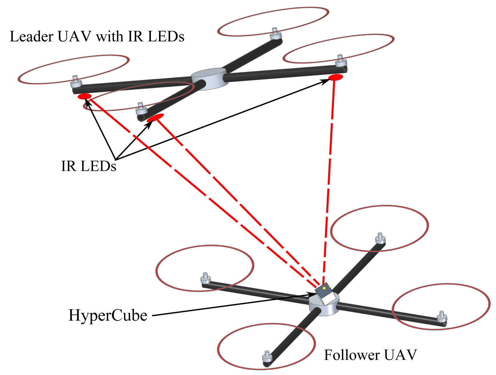
In this paper, we present a novel miniature optical sensor without any optics, called HyperCube, endowed with hyperacuity [15] for active IR LED marker tracking applications. The principle on which HyperCube is based was developed by Kerhuel et al. and detailed in [16,17]. In [16], hyperacuity was obtained at a very low cost. The Vibrating Optical Device for the Kontrol of Autonomous robots (VODKA) sensor was mounted onto a miniature aerial robot that was able to track a moving target accurately by exploiting the robot's uncontrolled random vibration as the source of its microscanning movement. In [17], an improved bio-inspired optical position sensing device was designed. Insect-based retinal microscanning movements were used to detect and locate contrasting objects, such as edges or bars. The active micro-vibrations imposed upon the retina endowed the sensor with hyperacuity. In this new paper, we designed a novel miniature bioinspired sensor where the mechanical vibration is replaced by a flickering LED. It is demonstrated that using only three photosensors with a sensitive area equal to 0.23 mm², we obtained hyperacuity by replacing the micro-movements with a modulation of infrared LEDs. The markers in use are off-the-shelf IR LEDs flickering at a high frequency (>1 kHz). We envision that this sensor could be used for cooperative flight, as presented in Figure 1.

The purpose of this paper is to present an alternative and a minimalistic solution involving three pixels for 3D localization with respect to IR markers. HyperCube assesses azimuth and elevation measurements of a pattern (planar object) composed of flickering IR LEDs. We also show the abilities of HyperCube to measure its relative position with respect to the markers. We propose a pose estimation system that consists of multiple flickering IR LEDs and a lightweight optical sensor. The LEDs are attached to a moving target, and the sensor provides angular measurements. We also show that the pose estimation is computationally inexpensive.

The paper is organized as follows: Section 2 details the principle of the sensor, the visual processing algorithm and its advantages. The principle of the sensor is discussed in Section 3. The experimental setup is presented in Section 4. Section 5 shows the experimental results.

2. Modeling the HyperCube Sensor

The prototype was built using off-the-shelf elements. Its volume is 1 cm³ and it weights 0.33 g. These characteristics make it inexpensive, light, small and power-lean.

2.1. Angular Sensitivity of the Photosensors

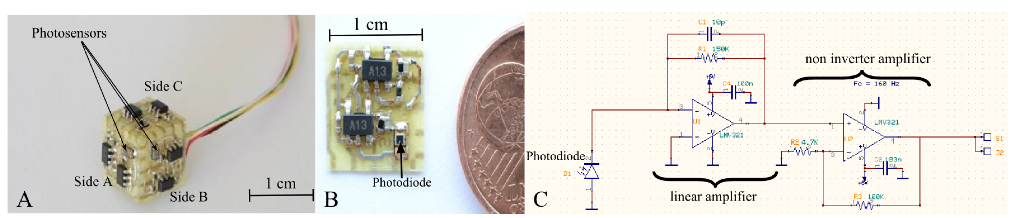
The HyperCube sensor is composed of three surface-mounted device (SMD) photodiodes (VISHAY TEMD7000). Each photodiode (or photosensor) is located on each side of the cube, as shown in Figure 2A. Thanks to this cubic assembly, the optical axes of each pair of photosensors are separated by an angle Δφ = 90°. On each side of the sensor, an analog circuit (Figure 2B) converts the output current of the photodiode into a proportional voltage thanks to a photoconductor electronic circuit (Figure 2C). The linear amplifier in Figure 2C is an analog low-pass filter with a cutoff frequency equal to 106 kHz. Considering the high gain given by the resistance of 150 kΩ, the linear amplifier aims at preventing the signal from oscillations.

HyperCube can extract two angular positions (azimuth and elevation) from the position of an object composed of several IR LEDs. The IR LEDs used in the experimental setup are the OSRAM SFH4232. Their spectrum has a maximum emissive power at a wavelength of 900 nm, which corresponds to the maximum of absorption of the photosensors. Thereafter, the IR LEDs will be considered as a point source. The signal processing used to estimate the elevation and azimuthal angles from the three HyperCube output signals runs in real time onboard a custom-made electronic board described in Section 2.2.

2.2. Model of the Photosensor Output Signal

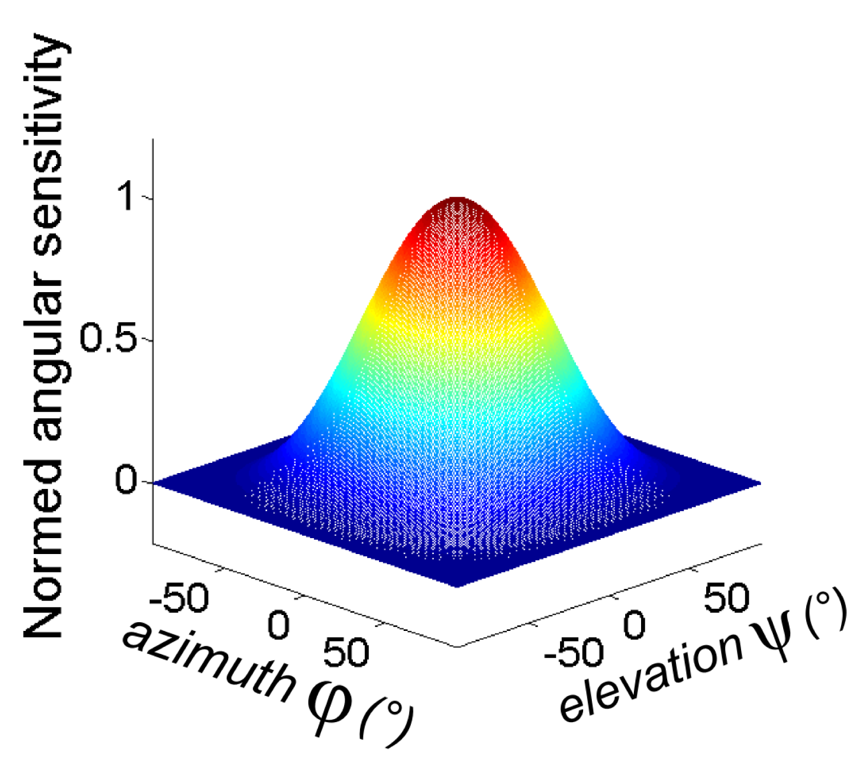
The cosine-like angular sensitivity function for each photosensor depends on the azimuth and elevation, as shown in Figure 3.

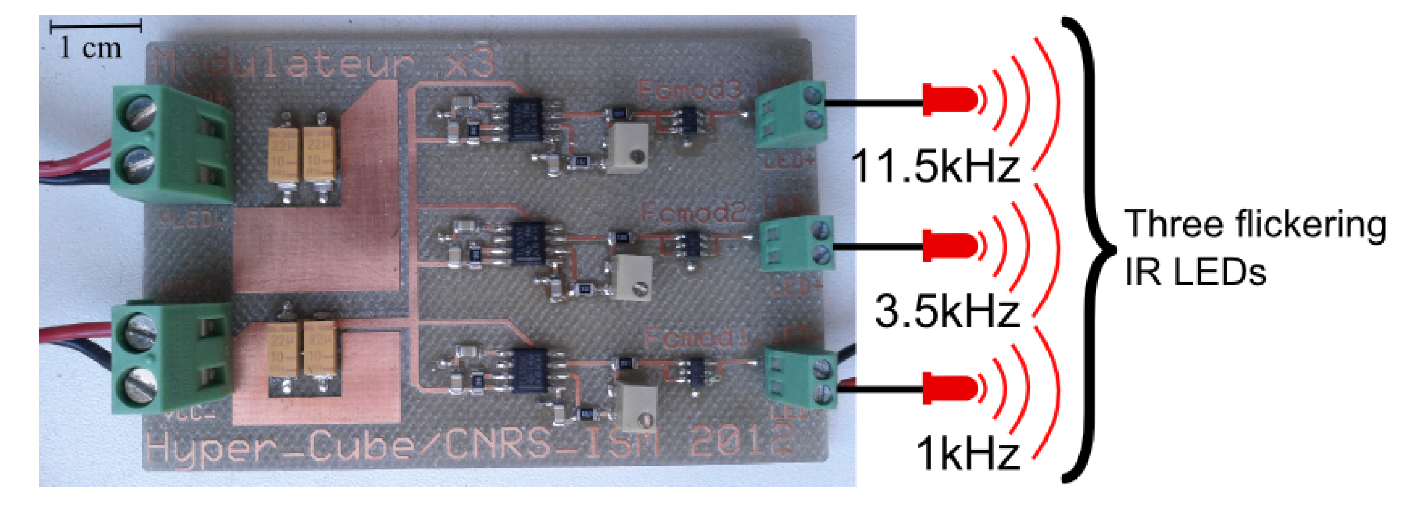
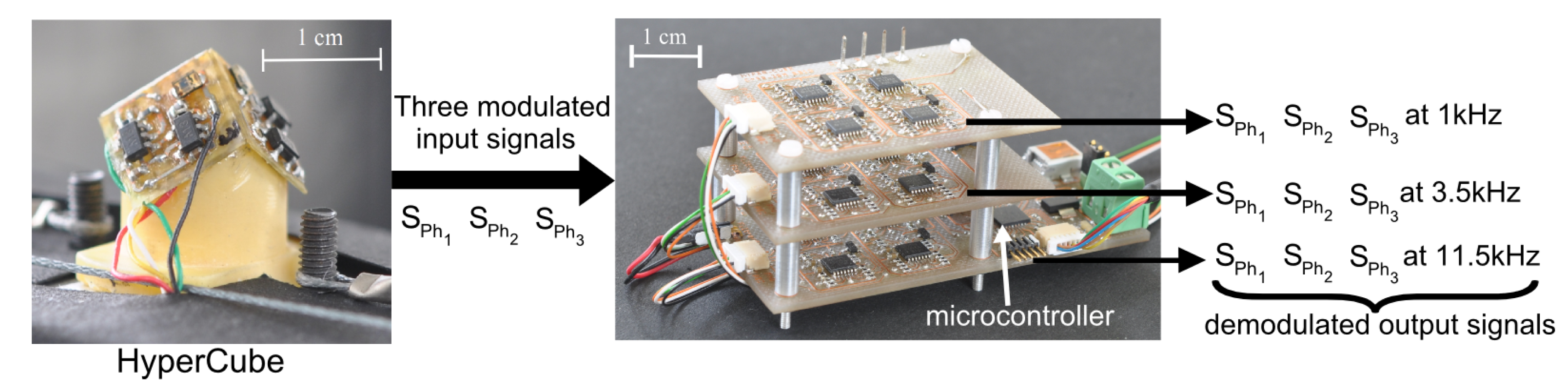
Each IR LED signal is modulated at a specific frequency f_i. The modulation is provided by a custom-made electronic board (Figure 4). The latter was designed to provide one specific modulation frequency f_i to each LED, such that f₁ = 1 kHz, f₂ = 3.5 kHz, f₃ = 11.5 kHz for the three separate IR LED emitters of the pattern. Then, an additional custom-made processing board (Figure 5) achieved the analog signal demodulation for each frequency f_i. To summarize, two electronic boards have been designed: the modulation of the LEDs is performed by the first board in Figure 4, and the second electronic board in Figure 5 performs the analog demodulation and the digital visual processing.

Once the three HyperCube output signals are demodulated, amplified and filtered by a low-pass filter at 100 Hz, one can approximate for each photosensor Ph_i and frequency f_i, the output signal S_phi,fi of HyperCube.

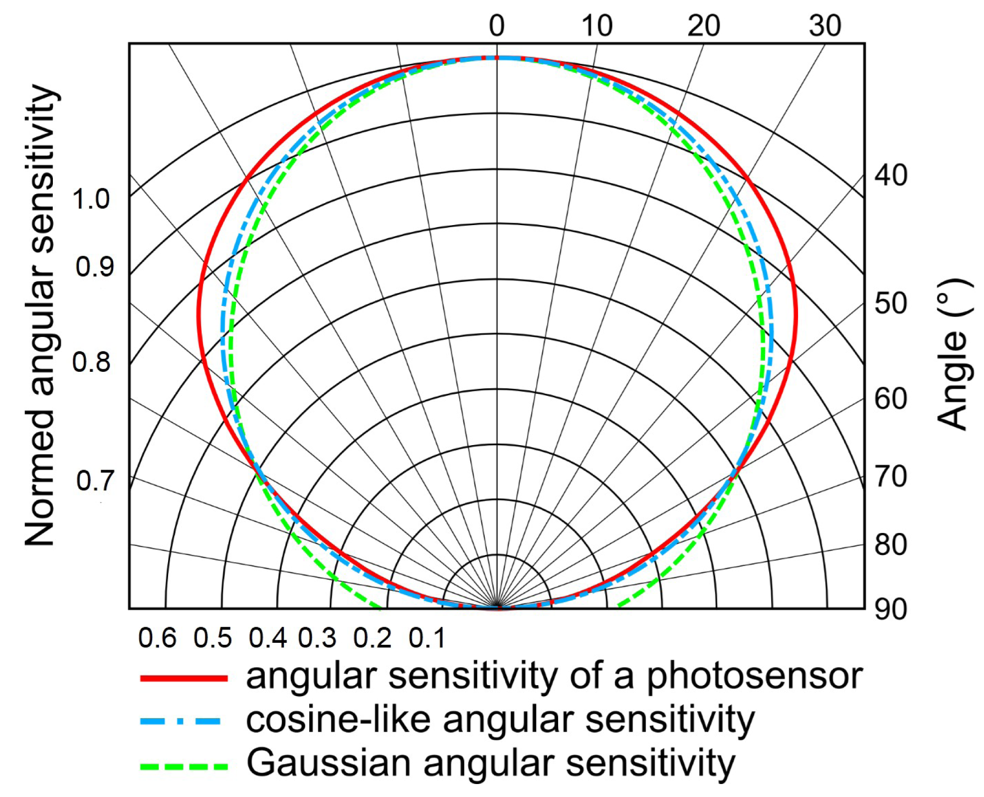
A Gaussian-like directivity function mimics the Gaussian angular sensitivity function of flies' photoreceptors [18,19]. The Gaussian-like angular sensitivity of each photosensor can be defined by the angle of acceptance, denoted Δρ. The angle Δρ is defined as the full width at half maximum, as depicted later in Figure 9. The Gaussian-like angular sensitivity of a photosensor is given by:

$$\sigma \left(\theta \right)=\frac{2\sqrt{\pi \mathit{\text{ln}}\left(2\right)}}{\pi \mathrm{\Delta }\rho }{e}^{-4\mathit{\text{ln}}\left(2\right)\left(\frac{{\theta }^2}{\mathrm{\Delta }{\rho }^2}\right)}$$

(1)

where θ is the angle between the photosensor's optical axis and that of a point light source. We also introduce the cosine-like angular sensitivity function σ, such that:

$$\sigma \left(\theta \right)=\{\begin{array}{cc}\mathit{cos}\left(\theta \right)& if\left|\theta \right|\le \frac{\pi }{2}\\ 0& \mathit{\text{else}}\end{array}$$

(2)

From Figure 6, the angular sensitivity of a photosensor as a blue dotted dashed line is compared to the Gaussian angular sensitivity given in Equation (1) as a green dashed line. One can note that the angular sensitivity of a photosensor does not strictly shape the Gaussian-like one and could also be approximated by a cosine-like angular sensitivity, which is plotted in red.

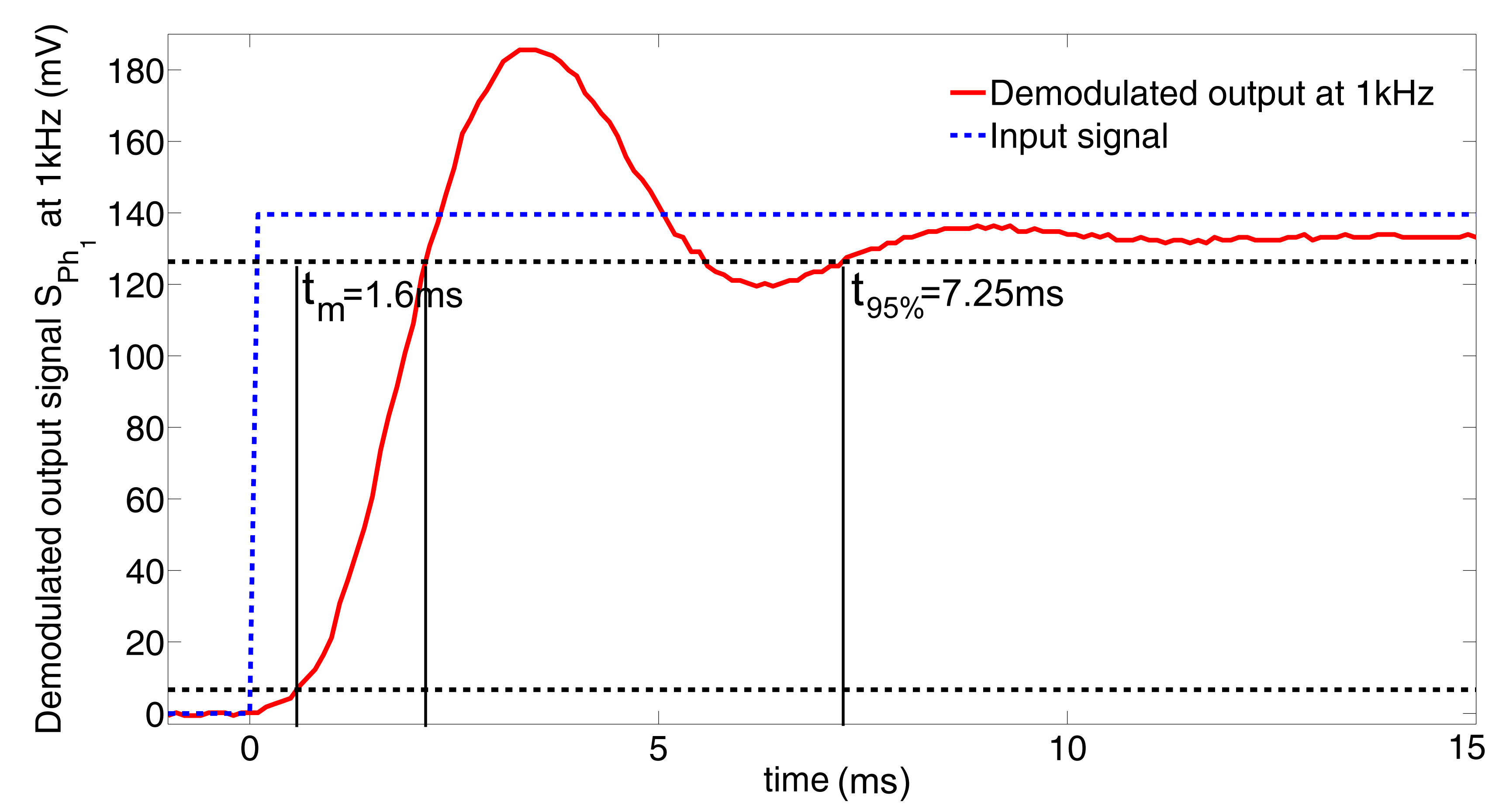
To characterize the dynamic response of the HyperCube sensor, we measured the demodulated output signal of a photosensor at 1 kHz in response to a step input. We turned on a modulated IR LED placed in front of the photosensor Ph₁, and we measured the demodulated output signal by means of the board, as shown in Figure 5. To precisely know the step time, the power input of the modulation electronic board (+3.3 V) is connected to a digital input of the microcontroller. The sampling frequency is 10 kHz. As depicted in Figure 7, the settling time t_95% is equal to 7.25 ms, and the rise time t_m is equal to 1.6 ms. Therefore, given these dynamic properties, the use of the HyperCube sensor could be relevant for MAV applications.

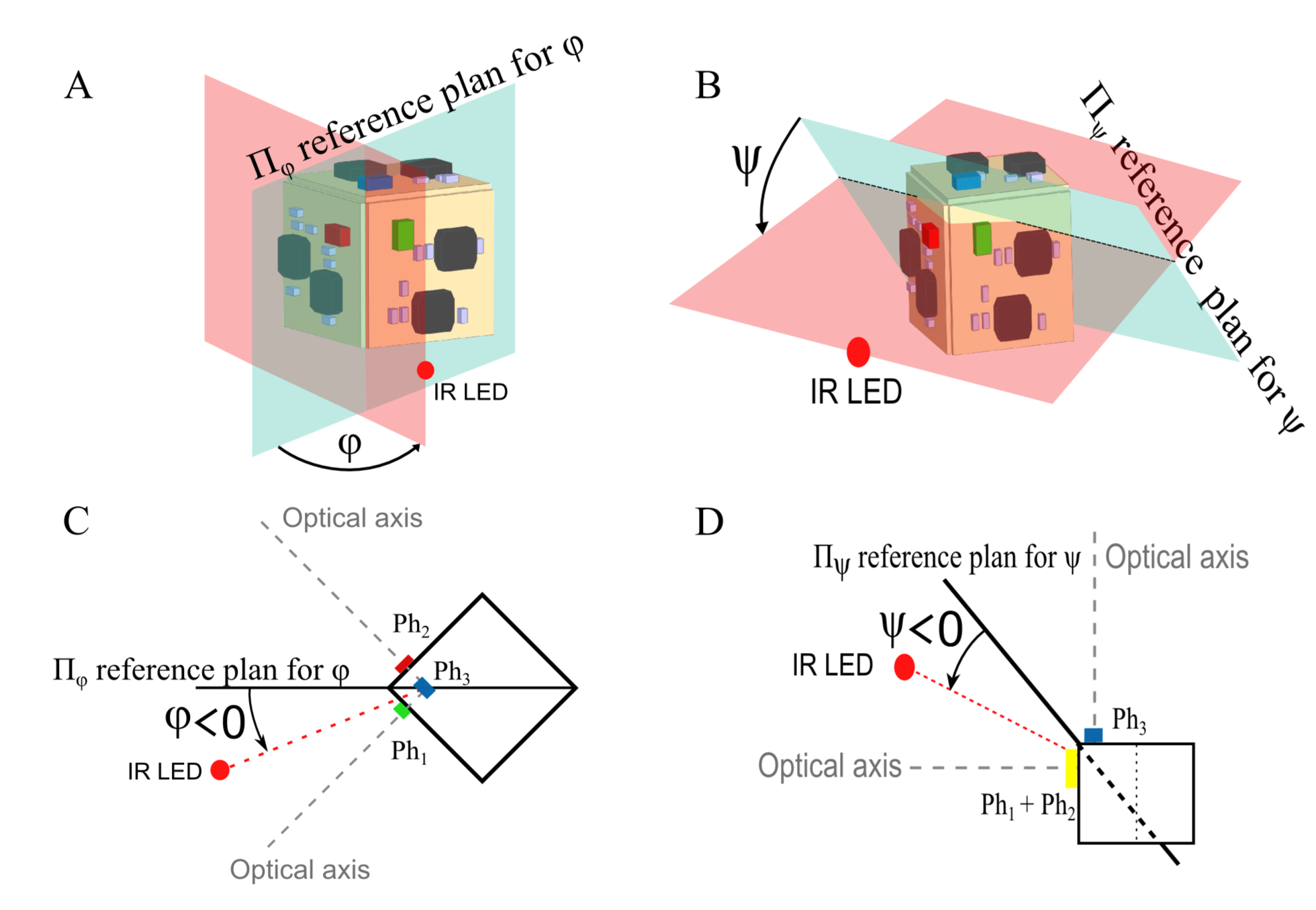
From Figure 8, the azimuth angle φ and the elevation angle ψ are defined.

Therefore, S_Phi,fi the output signal of the photodiode i is related to a specific flickering frequency f_i as follows:

$$\begin{array}{c}{S}_{P{h}_1,f_i}\left(\phi ,\psi \right)=A_{1,i}.\sigma \left(\phi -\frac{\pi }{4}\right).\sigma \left(\psi +\frac{\pi }{4}\right)\\ \text{if}\left|\phi -\frac{\pi }{4}\right|<\frac{\pi }{2}\text{and}\left|\psi +\frac{\pi }{4}\right|<\frac{\pi }{2}\text{else}{S}_{P{h}_1,f_i}\left(\phi ,\psi \right)=0\end{array}$$

(3)

$$\begin{array}{c}{S}_{P{h}_2,f_i}\left(\phi ,\psi \right)=A_{2,i}.\sigma \left(\phi +\frac{\pi }{4}\right).\sigma \left(\psi +\frac{\pi }{4}\right)\end{array}$$

(4)

$$\begin{array}{c}\text{if}\left|\phi +\frac{\pi }{4}\right|<\frac{\pi }{2}\text{and}\left|\psi +\frac{\pi }{4}\right|<\frac{\pi }{2}\text{else}{S}_{P{h}_2,f_i}\left(\phi ,\psi \right)=0\\ S_{P{h}_3,f_i}\left(\phi ,\psi \right)=A_{3,i}.\sigma \left(\phi \right).\sigma \left(\psi +\frac{\pi }{4}\right)\\ \text{if}\left|\phi \right|<\frac{\pi }{2}\text{and}\left|\psi -\frac{\pi }{4}\right|<\frac{\pi }{2}\text{else}{S}_{P{h}_3,f_i}\left(\phi ,\psi \right)=0\end{array}$$

(5)

With A_1,i, A_2,i, A_3,i, the gains of the photosensors Ph₁, Ph₂ or Ph₃ on each side of the HyperCube sensor. The index i refers to the frequencies 1 kHz, 3.5 kHz, 11.5 kHz. φ and ψ are the azimuth and elevation with respect the IR LED i.

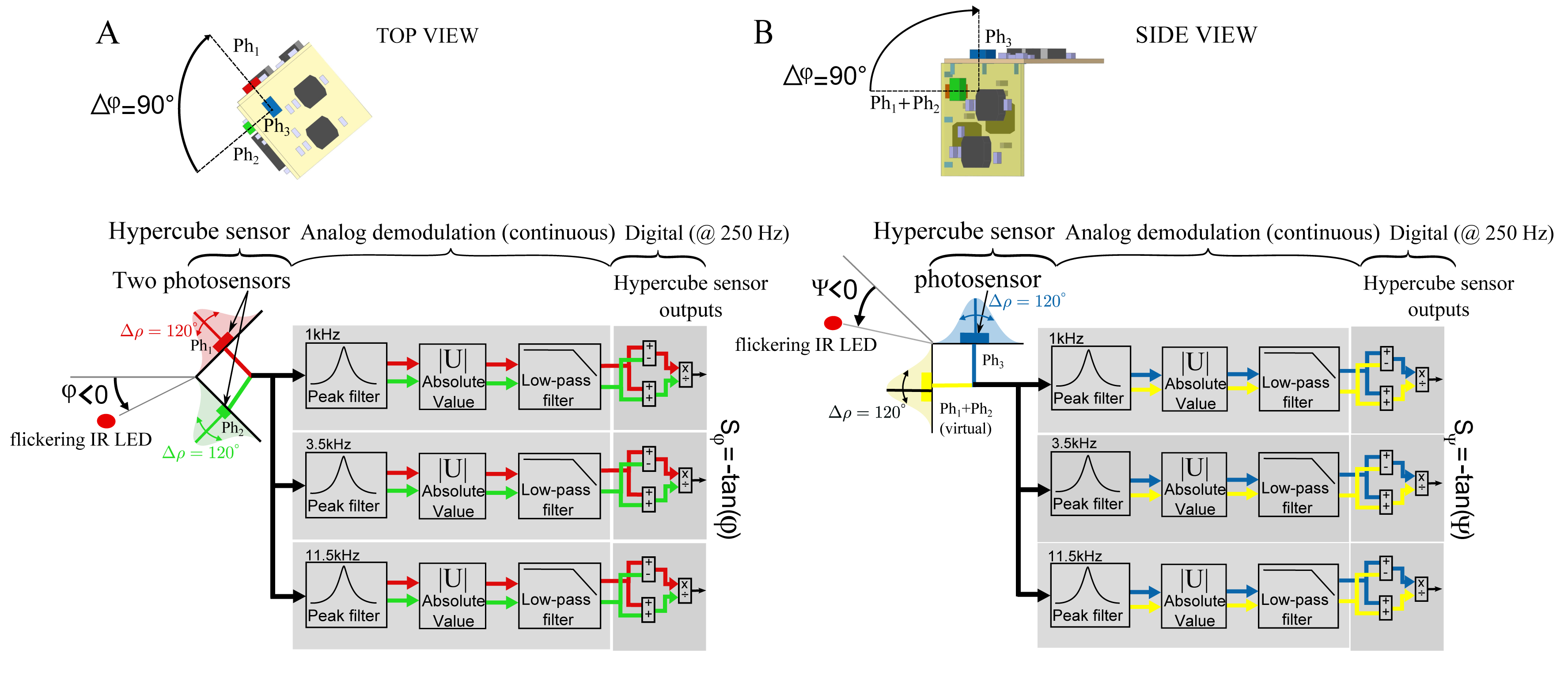
The three photosensor (photodiode) output signals are processed by a low-cost microcontroller from Microchip (dsPIC33FJ128GP802). As shown in Figure 9A,B, the digital processing operates at 250 Hz and computes the relative difference over the sum of two adjacent photosensor signals. For each frequency 1 kHz, 3.5 kHz and 11.5 kHz, respectively, a custom-made demodulation board was designed as depicted in Figure 5. Therefore, for each frequency f_i, a Sallen Key peak filter and a low pass filter with a cut off frequency equal to 100 Hz were chosen. The demodulated output signals , S_Ph2 and S_Ph3 were processed at 1kHz, 3.5 kHz and 11.5 kHz, respectively.

2.3. Advantages of HyperCube

HyperCube exhibits several advantages over other conventional sensors, like CMOS cameras, according to these following points:

• low cost: there is no optics; the angular position measurement relies only on the angular sensitivity of photodiodes, which is, in essence, non-uniform (cosine law) and only requires very inexpensive off-the-shelf electronic components.

• low computational resources: the measurements are the angular information; this does not require any image processing; a high refresh rate for the the same computational resource can easily be reached.

• small size: because of a low number of components, the sensor is light weight (0.33 g) and very compact (1cm³).

3. Principle of the HyperCube Sensor

3.1. Angle Reconstruction

Let us consider the azimuth angle φ. It is defined as the angle between the reference plane Π_φ (see Figure 8A) and a plane including the IR LED (see the red dotted line in Figure 8C). Π_φ is the mid-plane between the photosensors Ph₁ and Ph₂. The second plane includes the IR LED and the intersection between the optical axes of Ph₁ and Ph₂. In Figure 8A, the azimuth φ is presented in front view and in top view in Figure 8C.

The digital processing operated in the microcontroller with respect to the azimuth φ returns an output signal whose theoretical expression can be written as:

$$S_{\phi }=\frac{S_{p{h}_1}-S_{ph2}}{S_{p{h}_1}+S_{p{h}_2}}$$

(6)

Equation (6) gives the output signal, which results from two photosensors (Ph₁ and Ph₂, respectively), to obtain the ratio between the difference and the sum of the differentiated and demodulated photosensor signals. This expression reduces the common mode noise signal introduced by the artificial light. Moreover, the expression of Equation (6) results from previous studies carried out at the laboratory on hyperacute visual sensors based on active micro-movements applied to an artificial eye in [16,17]. It is worth noting that we obtained here hyperacuity by replacing the micro-movements with a modulation of IR LEDs. From Equation (6) using Equations (3) and (4), one can write:

$$S_{\phi }=\frac{A_1\sigma \left(\phi +\frac{\pi }{4}\right)·\sigma \left(\psi +\frac{\pi }{4}\right)-A_2\sigma \left(\phi -\frac{\pi }{4}\right)·\sigma \left(\psi +\frac{\pi }{4}\right)}{A_1\sigma \left(\phi +\frac{\pi }{4}\right)·\sigma \left(\psi +\frac{\pi }{4}\right)+A_2\sigma \left(\phi -\frac{\pi }{4}\right)·\sigma \left(\psi +\frac{\pi }{4}\right)}$$

(7)

A₁ and A₂ are the amplitudes of the signals delivered by the photosensors Ph₁ and Ph₂. If we assume A₁ = A₂, Equation (7) gives:

$$S_{\phi }=\frac{\mathit{cos}\left(\phi +\frac{\pi }{4}\right)-\mathit{cos}\left(\phi -\frac{\pi }{4}\right)}{\mathit{cos}\left(\phi +\frac{\pi }{4}\right)+\mathit{cos}\left(\phi -\frac{\pi }{4}\right)}$$

(8)

Therefore:

$$S_{\phi }=-\mathit{tan}\left(\phi \right)$$

(9)

The elevation angle ψ is defined as the angle between the reference plane Π_ψ (see Figure 8B) and a plane including the IR LED (see the red dotted line in Figure 8D). The second plane includes the IR LED and the intersection of the optical axes of the virtual photodiode (Ph₁ + Ph₂) and Ph₃. In Figure 8B, the elevation angle is presented in front view and in side view in Figure 8D.

The digital processing with respect to the elevation angle ψ involves a virtual photosensor (Ph₁ + Ph₂), which is the combination of Ph₁ and Ph₂. In the following, we introduce the signal S_Phvirtual delivered by the virtual photosensor:

$$\begin{array}{c}{S}_{P{h}_{\mathit{\text{virtual}}}}=S_{P{h}_1}+S_{P{h}_2}=A\sigma \left(\psi +\frac{\pi }{4}\right).\left[\sigma \left(\phi +\frac{\pi }{4}\right)+\sigma \left(\phi -\frac{\pi }{4}\right)\right]\\ S_{P{h}_{\mathit{\text{virtual}}}}=\{\begin{array}{cc}A\sigma \left(\psi +\frac{\pi }{4}\right)& if\left|\phi \right|<\frac{\pi }{4}\\ S_{P{h}_1}& if\frac{\pi }{4}<\phi <\frac{3\pi }{4}\\ S_{P{h}_2}& if-\frac{3\pi }{4}<\phi <-\frac{\pi }{4}\\ 0& \mathit{\text{else}}\end{array}\end{array}$$

Similarly to Equation (9), if we assume the amplitudes are such that A = A₁ = A₂ = A₃, the digital signal output for the elevation angle ψ gives: $S_{\psi }=\frac{S_{P{h}_{\mathit{\text{virtual}}}}-S_{Ph3}}{S_{P{h}_{\mathit{\text{virtual}}}}+S_{Ph3}}$. Using the definition of S_Phvirtual, one can write if $\left|\phi \right|<\frac{\pi }{4}$:

$$S_{\psi }=\frac{\sigma \left(\psi +\frac{\pi }{4}\right)-\sigma \left(\phi \right).\sigma \left(\psi -\frac{\pi }{4}\right)}{\sigma \left(\psi +\frac{\pi }{4}\right)-\sigma \left(\phi \right).\sigma \left(\psi -\frac{\pi }{4}\right)}$$

(10)

Considering the approximation of small angles for φ, σ (φ) ≃ 1, one can simplify:

$$S_{\psi }=\frac{\sigma \left(\psi +\frac{\pi }{4}\right)-\sigma \left(\psi -\frac{\pi }{4}\right)}{\sigma \left(\psi +\frac{\pi }{4}\right)+\sigma \left(\psi -\frac{\pi }{4}\right)}=\frac{\mathit{cos}\left(\psi +\frac{\pi }{4}\right)-\mathit{cos}\left(\psi -\frac{\pi }{4}\right)}{\mathit{cos}\left(\psi +\frac{\pi }{4}\right)+\mathit{cos}\left(\psi -\frac{\pi }{4}\right)}$$

Therefore:

$$S_{\psi }\simeq -\mathit{tan}\left(\psi \right)$$

(11)

3.2. Position Estimation

Given the signal outputs S_ψ and S_φ and one IR LED, the first step was to assess the relative position of the IR LED in the plane (X_LED,Y_LED) with respect to HyperCube. As described in the experimental setup presented in Section 4, if we assume Ẑ_LED is a priori known or assessed, using only angular measurements provided by HyperCube, the relative position of the IR LED with respect the sensor can be estimated such as:

$${\widehat{X}}_{\mathit{\text{LED}}}=-\mathit{tan}\left(\phi \right){\widehat{Z}}_{\mathit{\text{LED}}}$$

(12)

$${\widehat{Y}}_{\mathit{\text{LED}}}=-\mathit{tan}\left(\psi \right){\widehat{Z}}_{\mathit{\text{LED}}}$$

(13)

where φ < 0 and ψ < 0 as defined in Figure 9A,B.

The experimental setup detailed in Section 4 justifies the approximation of the small angles. Therefore, one can assume that:

$${\widehat{X}}_{\mathit{\text{LED}}}=-\phi ·{\widehat{Z}}_{\mathit{\text{LED}}}$$

(14)

$${\widehat{Y}}_{\mathit{\text{LED}}}=-\psi ·{\widehat{Z}}_{\mathit{\text{LED}}}$$

(15)

4. Experimental Setup

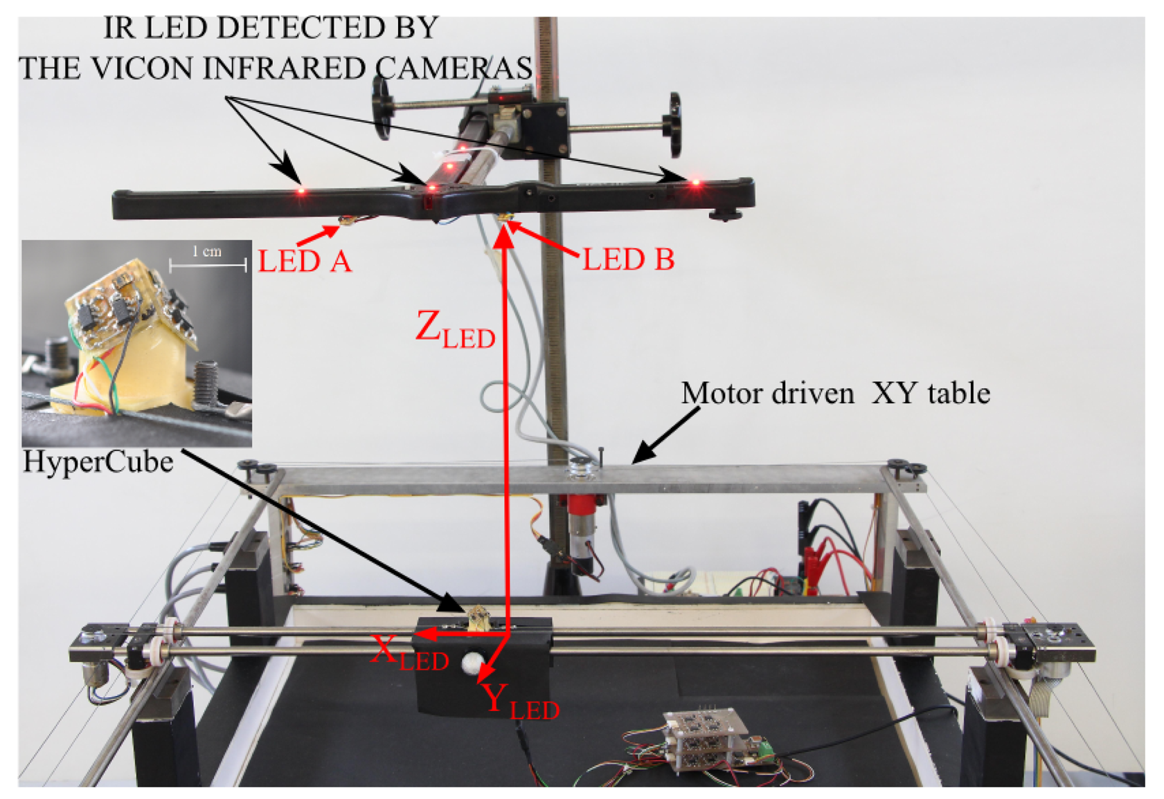
In this work, we aimed at demonstrating that the estimation of the relative position of an IR LED with respect to HyperCube can be achieved by means of angular measurements. The experimental setup is composed of a motor-driven XY table, as shown in Figure 10. We oriented HyperCube so that it was pointing upward. HyperCube can move along the X and Y directions thanks to two DC motors.

Two incremental encoders measure the HyperCube position along the X and Y directions. In the initial conditions, which define the origin of the inertial frame, an IR LED is located just above HyperCube at a height Z_LED = 300 mm. As an absolute sensor's position of reference, a motion capture system provided by the company VICON was used for measuring the ground truth, i.e., the precise absolute position of HyperCube. The tracking system is equipped with 17 IR cameras and IR active markers that are pointed upward, as depicted in Figure 10. The HyperCube position of reference was therefore measured in real time with a sub-millimetric precision.

4.1. Calibration

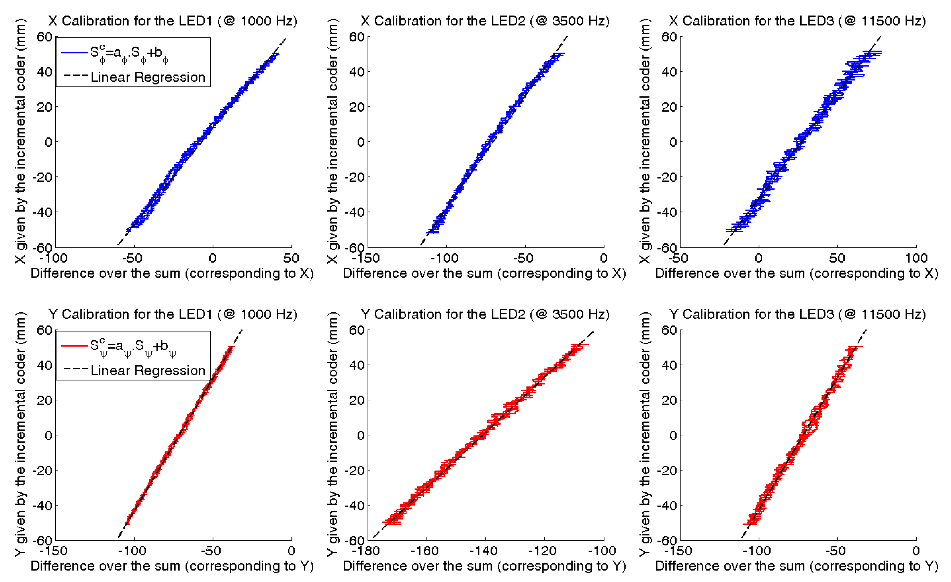
In this work, we consider that the HyperCube sensor can move in a range of [−50 mm; +50 mm] in both X and Y directions. Given Z_LED = 300 mm, one can assume that the angles are small enough to write from Equation (9) S_φ = −tan(φ) ⋍ −φ for azimuth and from Equation (11) S_ψ = −tan(ψ) ⋍ −ψ for elevation. As shown in the experimental setup in Figure 10, we theoretically have $S_{\phi }=-\mathit{tan}\phi =\frac{X_{\mathit{\text{LED}}}}{Z_{\mathit{\text{LED}}}}$ and $S_{\psi }=-\mathit{tan}\psi =\frac{Y_{\mathit{\text{LED}}}}{Z_{\mathit{\text{LED}}}}$, where X_LED, Y_LED and Z_LED are the relative position of the IR LED to the HyperCube sensor. The positions of reference X_LED, Y_LED and Z_LED are provided by the tracking system VICON.

The calibration consists of adjusting the HyperCube outputs S_φ and S_ψ to the ratios $\frac{X_{\mathit{\text{LED}}}}{Z_{\mathit{\text{LED}}}}$ and $\frac{Y_{\mathit{\text{LED}}}}{Z_{\mathit{\text{LED}}}}$. To this aim, the calibration curves shown in Figure 11 are plotted. We note that the HyperCube outputs are linear in the observed range [−50 mm; +50 mm]. Linear regression computes the slope (a_φ, a_ψ) and the offset (b_φ, b_ψ) by fitting each curve with a linear model. These coefficients calibrate the HyperCube outputs $S_{\phi }^c$ and $S_{\psi }^c$, such that: $S_{\phi }^c=a_{\phi }.S_{\phi }+b_{\phi }=\frac{X_{\mathit{\text{LED}}}}{Z_{\mathit{\text{LED}}}}=-\phi$ and $S_{\psi }^c=a_{\psi }.S_{\psi }+b_{\psi }=\frac{X_{\mathit{\text{LED}}}}{Z_{\mathit{\text{LED}}}}=-\psi$. Figure 11 presents the calibration results for each IR LED in both the X and Y directions. The sensor's outputs are linear in the range [−50 mm; +50 mm] with respect to the origin.

The calibration validation protocol takes Z_LED = 300 mm. The estimated positions X̂_LED and Ŷ_LED of the IR LED were compared to the references X_LED and Y_LED provided by the VICON system.

4.2. Height Estimation

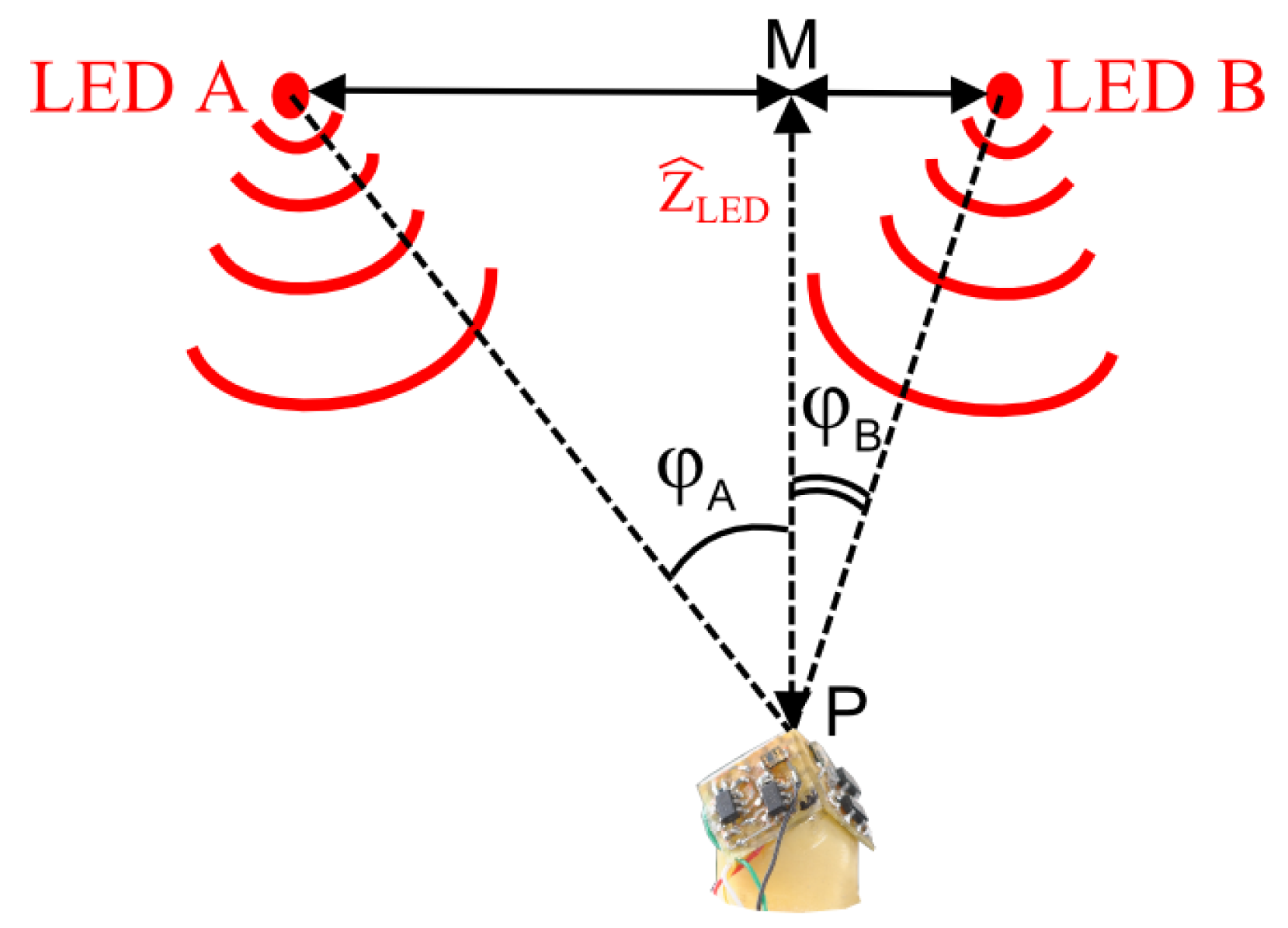
Form the experimental setup described in Figure 10 and given the signal outputs S_ψ and S_φ and two IR LEDs, one can assess the height Z_LED between the sensor and two IR LEDs A and B.

The assessed height Ẑ_LED is given by the relation: ${\widehat{Z}}_{\mathit{\text{LED}}}=\frac{AB}{\mathit{tan}\left({\phi }_A\right)+\mathit{tan}\left({\phi }_B\right)}$ where AB is the distance between the LEDs A and B. φ_A and φ_B are the azimuthal angles given by HyperCube for the LEDs A and B. In the configuration described in Figure 12, Y_LED = 0 (i.e., ABPis orthogonal to the horizontal plane that intersects HyperCube).

5. Experimental Position Estimation in 2D

In this section, we used a single IR LED and HyperCube for each experiment.

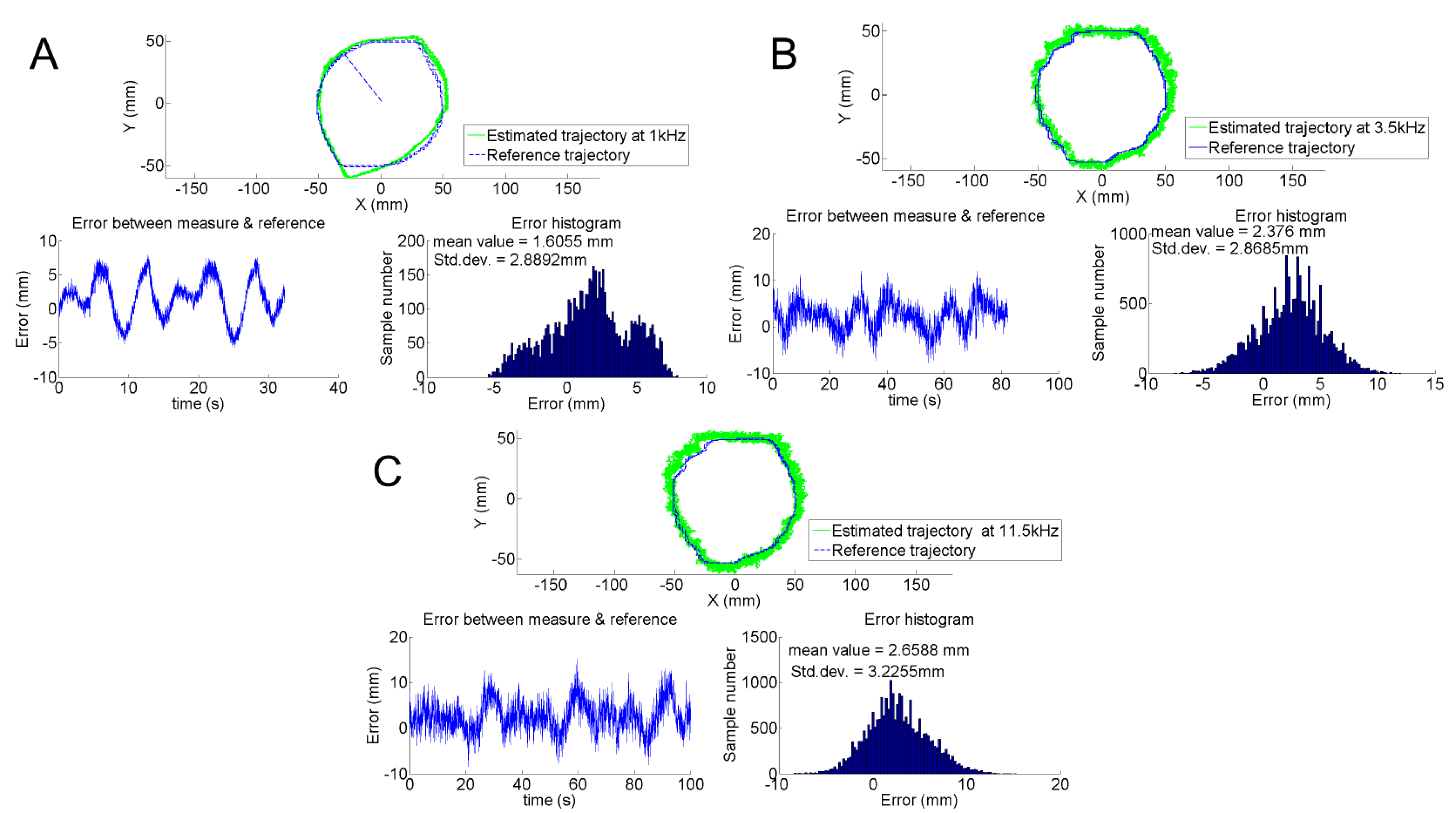
We compared the estimation to HyperCube positions assessed by the tracking system for three different modulation frequencies. For the IR LED that flickers at 1 kHz, Figure 13A shows the plots of the reference trajectory as a dashed line and the trajectory depicted by HyperCube as a solid line. The trajectory is a circular path with a radius of 50 mm in the XY plane with Z_LED = 300 mm. The distance between reference and estimated trajectories was also plotted. The histogram of the error gives a mean value μ = 1.6 mm and a standard deviation σ = 2.8 mm. We noted that the noise at 1 kHz for the demodulation was lower than the noise at 3.5 kHz and 11.5 kHz, as shown in Figure 13B,C. The higher levels of noise at 3.5 kHz and 11.5 kHz than the one at 1 kHz are due to the use of different operational amplifiers (TI OPA4322 and TIOPA4342) for the analog demodulation. Figure 13A-C highlight that the HyperCube sensor provides useful measurements to accurately estimate the dynamic relative position of an IR LED in the XY plane.

To reduce the measurement noise, the digital signal outputs given by the HyperCube sensor were filtered by a Kalman filter. The system is described in a state space form as follows:

$$x_{k+1}=F{x}_k+v_k,$$

(16)

$$y_k=C{x}_k+w_k\text{with}k\in \mathbb{N}$$

(17)

where the state x_k = [X_k Ẋ_k]^T describes the position X_k and the velocity Ẋ_k at the time instant t_k. w_k and v_k are the state and measurement white noise with known and constant covariance matrices W and V, respectively. They are supposed to be mutually uncorrelated. $F=\left[\begin{array}{cc}1& T_e\\ 0& 1\end{array}\right]$ is the state transition matrix, C = [1 0] the observation matrix. In practice, we choose the covariance matrices as follows $V={\sigma }_{\mathit{\text{meas}}}^2\left[\begin{array}{cc}1& 0\\ 0& 1\end{array}\right]$ and $W={\sigma }_{\mathit{\text{proc}}}^2\left[\begin{array}{cc}1& 0\\ 0& 1\end{array}\right]$ where σ_meas and σ_proc are the standard deviations of the measurement noise and the state noise, respectively.

A linear Kalman filter was also implemented for the state estimation along the Y direction.

5.1. Experimental Height Estimation

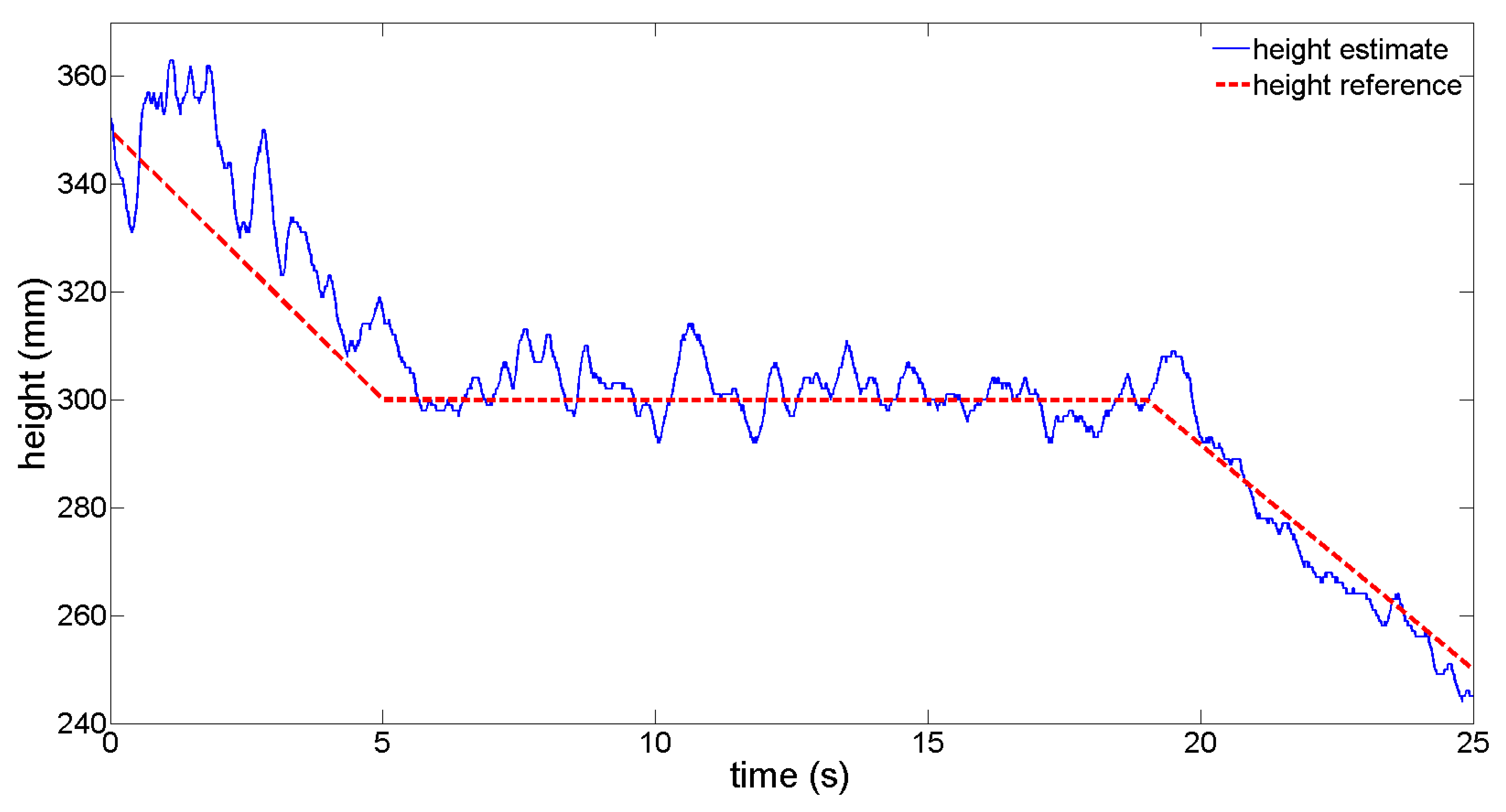
As described in Section 4.2, the height between the HyperCube sensor and a pair of IR LEDs was estimated. Thanks to the angular measurements using three flickering IR LEDs, one can reduce the measurement noise. The height estimation precision is therefore increased. The mean of the height estimate Ẑ̅ is written as:

$$\overline{\widehat{Z}}=\frac{{\widehat{Z}}_{\mathit{\text{LED}}1,2}+{\widehat{Z}}_{\mathit{\text{LED}}2,3}+{\widehat{Z}}_{\mathit{\text{LED}}1,3}}{3}$$

(18)

where Ẑ_LED1,2, Ẑ_LED2,3 and Ẑ_LED1,3 are the height estimated by the pairs (1,2), (2,3) and (1,3), respectively. The height of the IR LEDS was modified, while the position of the HyperCube sensor was fixed in the XY plane. Using each pair of IR LEDs, the height estimation was computed on-line. From Figure 14, the height estimation as a solid line is precise around 300 mm with respect to the reference height as a dashed line.

In Figure 15, for different pairs of IR LEDs, we plotted the evolution of the height estimation while the sensor was moving relatively to the center of the pair of IR LEDs. We note from Figure 15 that the height estimation depends on the position (X_LED, Y_LED) of the sensor. The estimation error can vary up to 50 mm.

The estimation remains better with the pair of IR LEDs (1 kHz and 3.5 kHz) than with the others.

5.2. IR LED Position Tracking in 2D

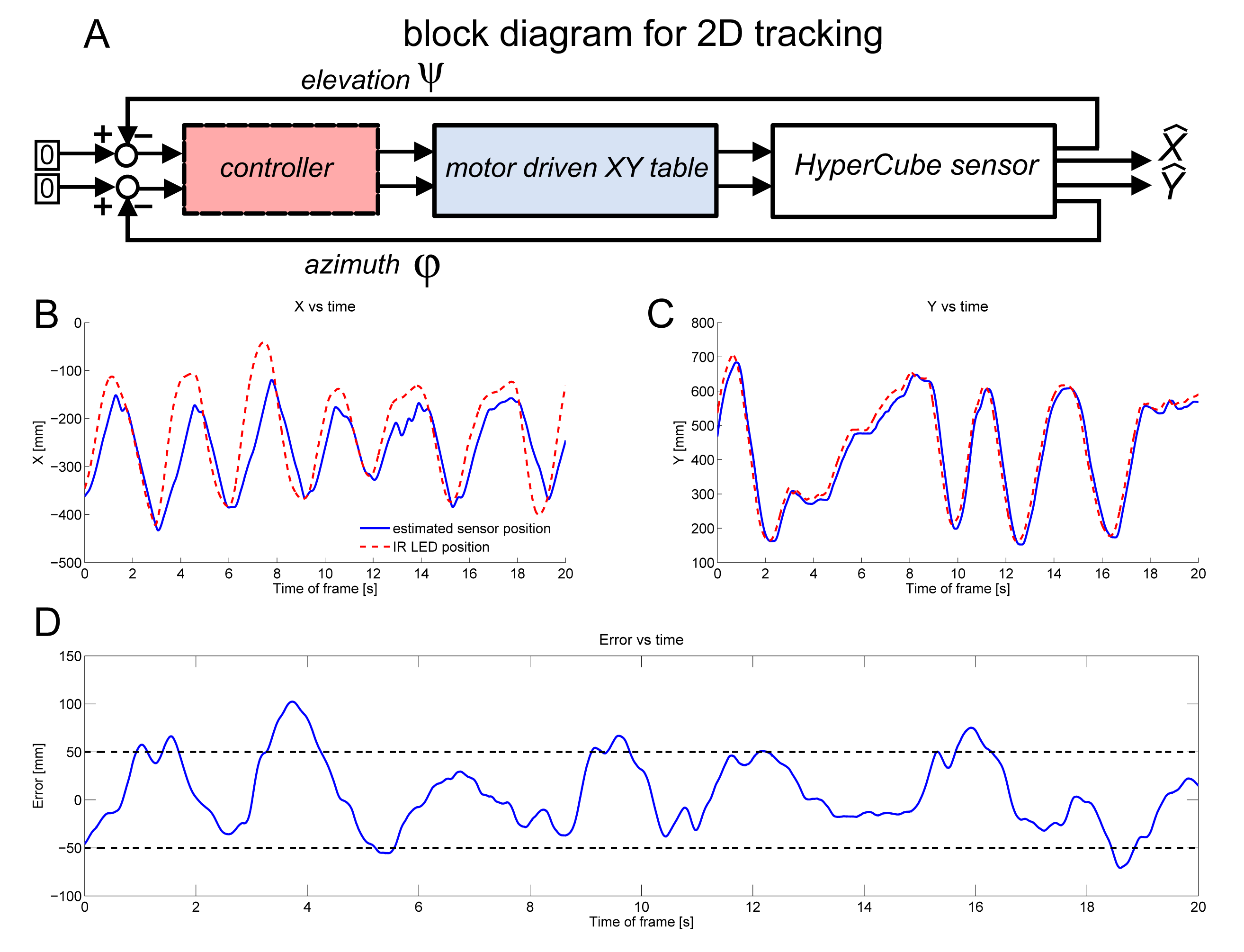
In this section, HyperCube measurements, which consist of azimuth φ and elevation ψ, feed the controller that aims at tracking a moving IR LED in the plane. A Smith predictor with proportional and integral actions was designed and implemented to ensure the good stability of the linear displacement of HyperCube despite the time lag inherent to the visual processing algorithm. Figure 16A shows the block diagram of the closed loop system with the assessed angles φ and ψ. In Figure 16B,C, estimated positions versus time are plotted. The tracking system gives the reference trajectory.

As shown in Figure 16B,C, the position tracking was accurate. The tracking error plotted in the Figure 16D shows that the error ranges within ±5 cm. Nevertheless, one can note in Figure 16B that there is an error between the estimated and the reference values due to a saturation of the motor of the X axis. Thanks to a fast motor for controlling the Y axis, HyperCube was able to follow faithfully the moving pattern. In Figure 16C, the HyperCube sensor perfectly tracks the moving IR LED along the Y axis.

6. Conclusions

We designed and presented the HyperCube sensor. It is a cubic, miniature and low-cost sensing device able to track active markers without any optics. The system discussed has the following key features:

• It provides azimuth and elevation and is able to assess the angular position of three blinking IR LEDs at specific frequencies: 1 kHz, 3.5 kHz and 11.5 kHz.

• The estimation is achieved by a computationally-inexpensive signal processing of the low-amplitude and high-frequency signal transmitted by the three photodiodes placed on each side of the cube.

• Experimental results showed that for the position estimation and the position tracking in 2D, this miniature device is very efficient. It also features promising results in terms of distance estimation, as well.

Nevertheless, the prototype developed reveals some limitations with respect to the range of pose estimation, but it is well adapted for proximal localization (up to 30 cm). In addition, the size of the demodulation electronic board could be easily reduced. As a conclusion, the HyperCube sensor is a promising sensing device for proximal localization applications and could equip UAVs or MAVs. The short-term outlook consists of improving the range of sensitivity of HyperCube using silicon photodiodes, which are specifically designed for precision photometry and feature a high sensitivity, a high-speed response and low noise.

References

- Breitenmoser, A.; Kneip, L.; Siegwart, R. A monocular vision-based system for 6D relative robot localization. Proceedings of the 2011 IEEE/RSJ International Conference on Intelligent Robots and Systems (IROS), San Francisco, CA, USA, 25–30 September 2011; pp. 79–85.
- Audette, R.; Balthazaar, J.; Dunk, C.; Zelek, J. A Stereo-Vision System for the Visually Impaired; University of Guelph: Guelph, ON, Canada, 2000. [Google Scholar]
- Cardin, S.; Vexo, F.; Thalmann, D. Wearable system for mobility improvement of visually impaired people. Vis. Comp. J. 2006, 23, 109–118. [Google Scholar]
- Ijaz, F.; Yang, H.K.; Ahmad, A.; Lee, C. Indoor positioning: A review of indoor ultrasonic positioning systems. Proceedings of the 15th International Conference on Advanced Communication Technology (ICACT), PyeongChang, Korea, 27–30 Janunary 2013; pp. 1146–1150.
- Aloui, N.; Raoof, K.; Bouallegue, A.; Letourneur, S.; Zaibi, S. Performance evaluation of an acoustic indoor localization system based on a fingerprinting technique. EURASIP J. Adv. Signal Process. 2014, 2014. [Google Scholar] [CrossRef]
- Dobrzynski, M.; Pericet-Camara, R.; Floreano, D. Vision tape—A flexible compound camera for motion detection and proximity estimation. IEEE Sens. J. 2012, 12, 1131–1139. [Google Scholar]
- Floreano, D.; Pericet-Camara, R.; Viollet, S.; Ruffier, F.; Brückner, A.; Leitel, R.; Buss, W.; Menouni, M.; Expert, F.; Juston, R.; et al. Miniature curved artificial compound eyes. Proc. Natl. Acad. Sci. USA 2013, 110, 9267–9272. [Google Scholar]
- Censi, A.; Strubel, J.; Brandli, C.; Delbruck, T.; Scaramuzza, D. Low-latency localization by active LED markers tracking using a dynamic vision sensor. Proceedings of the 2013 IEEE/RSJ International Conference on Intelligent Robots and Systems (IROS), Tokyo, Japan, 3–7 November 2013; pp. 891–898.
- Lichtsteiner, P.; Posch, C.; Delbruck, T. A 128× 128 120 dB 15 μ s latency asynchronous temporal contrast vision sensor. IEEE J. Sol. State Circuits 2008, 43, 566–576. [Google Scholar]
- Faessler, M.; Mueggler, E.; Schwabe, K.; Scaramuzza, D. A monocular pose estimation system based on Infrared LEDs. Proceedinds of the IEEE International Conference on Robotics and Automation (ICRA), Hong Kong, China, 31 May–7 June 2014.
- Roberts, J.; Stirling, T.; Zufferey, J.C.; Floreano, D. 3-D relative positioning sensor for indoor flying robots. Auton. Robots 2012, 33, 5–20. [Google Scholar]
- Wenzel, K.; Masselli, A.; Zell, A. Visual tracking and following of a quadrocopter by another quadrocopter. 4993–4998.
- Etter, W.; Martin, P.; Mangharam, R. Cooperative flight guidance of autonomous unmanned aerial vehicles. Proceedings of the 2nd Internation Workshop on Networks of Cooperating Objects, Chicago, IL, USA, 11–12 April 2011.
- Masselli, A.; Zell, A. A novel marker based tracking method for position and attitude control of MAVs. Proceedings of International Micro Air Vehicle Conference and Flight Competition (IMAV), Braunschweig, Germany, 3–6 July 2012.
- Westheimer, G. Visual hyperacuity, Progress in Sensory Physiology; Springer: Berlin, Germany, 1981; pp. 1–30. [Google Scholar]
- Kerhuel, L.; Viollet, S.; Franceschini, N. The VODKA sensor: A bio-inspired hyperacute optical position sensing device. IEEE Sens. J. 2012, 12, 315–324. [Google Scholar]
- Juston, R.; Kerhuel, L.; Franceschini, N.; Viollet, S. Hyperacute edge and bar detection in a bioinspired optical position sensing device. IEEE/ASME Trans. Mechatron. 2013, 19, 1025–1034. [Google Scholar]
- Götz, K. Optomotorische Untersuchung des visuellen Systems einiger Augenmutanten der Fruchtfliege. Drosophila. Biol. Cybern. 1964, 2, 77–92. [Google Scholar]
- Stavenga, D. Angular and spectral sensitivity of fly photoreceptors. II. dependence on facet lens F-number and rhabdomere type in Drosophila. J. Comp. Phys. A 2003, 189, 189–202. [Google Scholar]
© 2015 by the authors; licensee MDPI, Basel, Switzerland This article is an open access article distributed under the terms and conditions of the Creative Commons Attribution license (http://creativecommons.org/licenses/by/4.0/).
Share and Cite
Raharijaona, T.; Mignon, P.; Juston, R.; Kerhuel, L.; Viollet, S. HyperCube: A Small Lensless Position Sensing Device for the Tracking of Flickering Infrared LEDs. Sensors 2015, 15, 16484-16502. https://doi.org/10.3390/s150716484
Raharijaona T, Mignon P, Juston R, Kerhuel L, Viollet S. HyperCube: A Small Lensless Position Sensing Device for the Tracking of Flickering Infrared LEDs. Sensors. 2015; 15(7):16484-16502. https://doi.org/10.3390/s150716484
Chicago/Turabian StyleRaharijaona, Thibaut, Paul Mignon, Raphaël Juston, Lubin Kerhuel, and Stéphane Viollet. 2015. "HyperCube: A Small Lensless Position Sensing Device for the Tracking of Flickering Infrared LEDs" Sensors 15, no. 7: 16484-16502. https://doi.org/10.3390/s150716484
APA StyleRaharijaona, T., Mignon, P., Juston, R., Kerhuel, L., & Viollet, S. (2015). HyperCube: A Small Lensless Position Sensing Device for the Tracking of Flickering Infrared LEDs. Sensors, 15(7), 16484-16502. https://doi.org/10.3390/s150716484