
Evaluation of a Cubature Kalman Filtering-Based Phase Unwrapping Method for Differential Interferograms with High Noise in Coal Mining Areas


Abstract
:1. Introduction
2. Phase Unwrapping Theory and Local Phase Slope Estimation
2.1. Phase Unwrapping Theory
2.2. Phase Slope Estimation
3. Cubature Kalman Filtering Based Phase Unwrapping
3.1. System Model for Phase Unwrapping
3.1.1. State-Space Equation
3.1.2. Observation Equation
3.2. CKF Phase Unwrapping (CKFPU) Algorithms
3.2.1. One-Dimensional CKFPU Algorithm
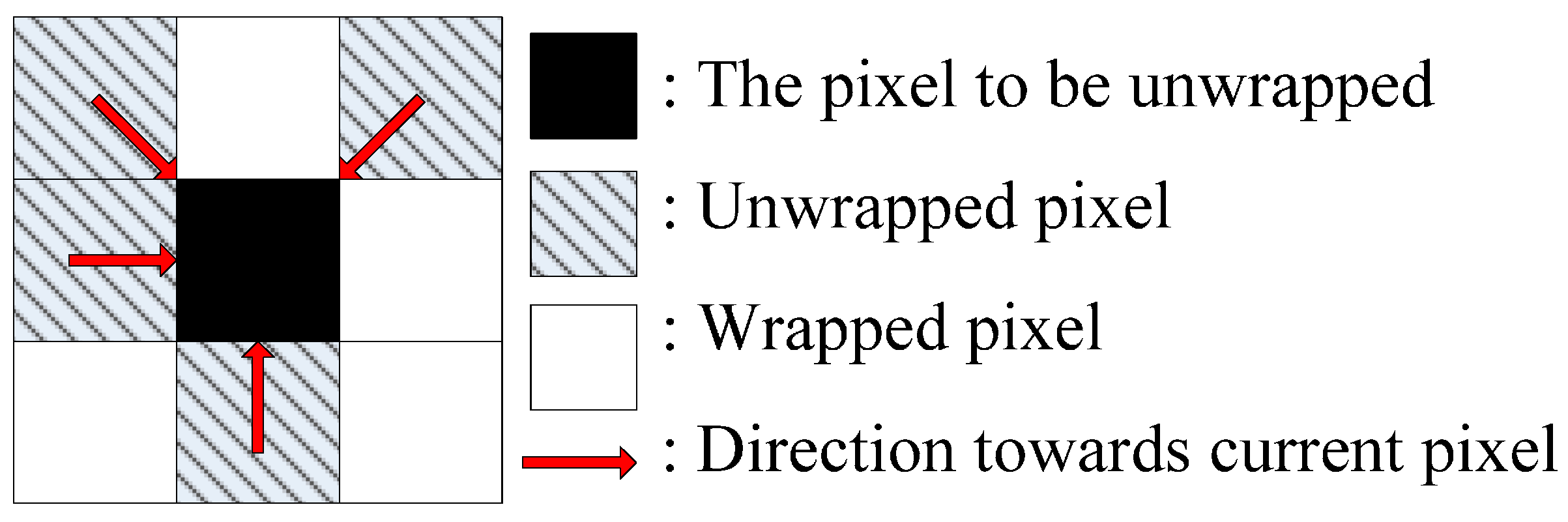
3.2.2. Two-Dimensional CKFPU Algorithm
3.3. The Main Factors Affecting CKFPU Performance
3.3.1. Number of Multi-Looks
3.3.2. Quality Indexes for Guiding Path Tracking
Maximum Coherence
Phase Derivative Variance
Fisher Distance
4. Experiments
4.1. Dataset Introduction and DInSAR Processing Strategy
4.1.1. Dataset Introduction

| Parameters | Values |
|---|---|
| Frequency | 9.6 GHZ |
| Wavelength | 3.1 cm |
| Polarisation | HH |
| Swath Width | 50 km |
| Incidence Angle | ~26° |
| Range Pixel Spacing | 0.9 m |
| Azimuth Pixel Spacing | 1.9 m |
| Orbit Repeat Cycle | 11 days |
| Precise Orbit Accuracy | ~10 cm |
| Datasets | Target Working Face | Master | Slave | Perpendicular Baseline B⊥/m | Temporal Baseline BT/day |
|---|---|---|---|---|---|
| A | 18a203 | 4 January 2013 | 15 January 2013 | −103.3 | 11 |
| B | 52304 | 2 April 2013 | 24 April 2013 | −107.2 | 22 |
| C | 18a203 | 16 September 2012 | 27 September 2012 | −3 | 11 |
| 27 September 2012 | 8 October 2012 | −7.2 | 11 | ||
| 8 October 2012 | 19 October 2012 | −70.2 | 11 | ||
| 19 October 2012 | 10 November 2012 | −30.5 | 22 | ||
| 10 November 2012 | 21 November 2012 | 62.2 | 11 | ||
| 21 November 2012 | 2 December 2012 | 160.7 | 11 | ||
| 2 December 2012 | 13 December 2012 | −36.3 | 11 | ||
| 13 December 2012 | 24 December 2012 | −99.8 | 11 |

4.1.2. DInSAR Processing Strategy
4.2. Results and Analysis
4.2.1. Case 1
4.2.2. Case 2
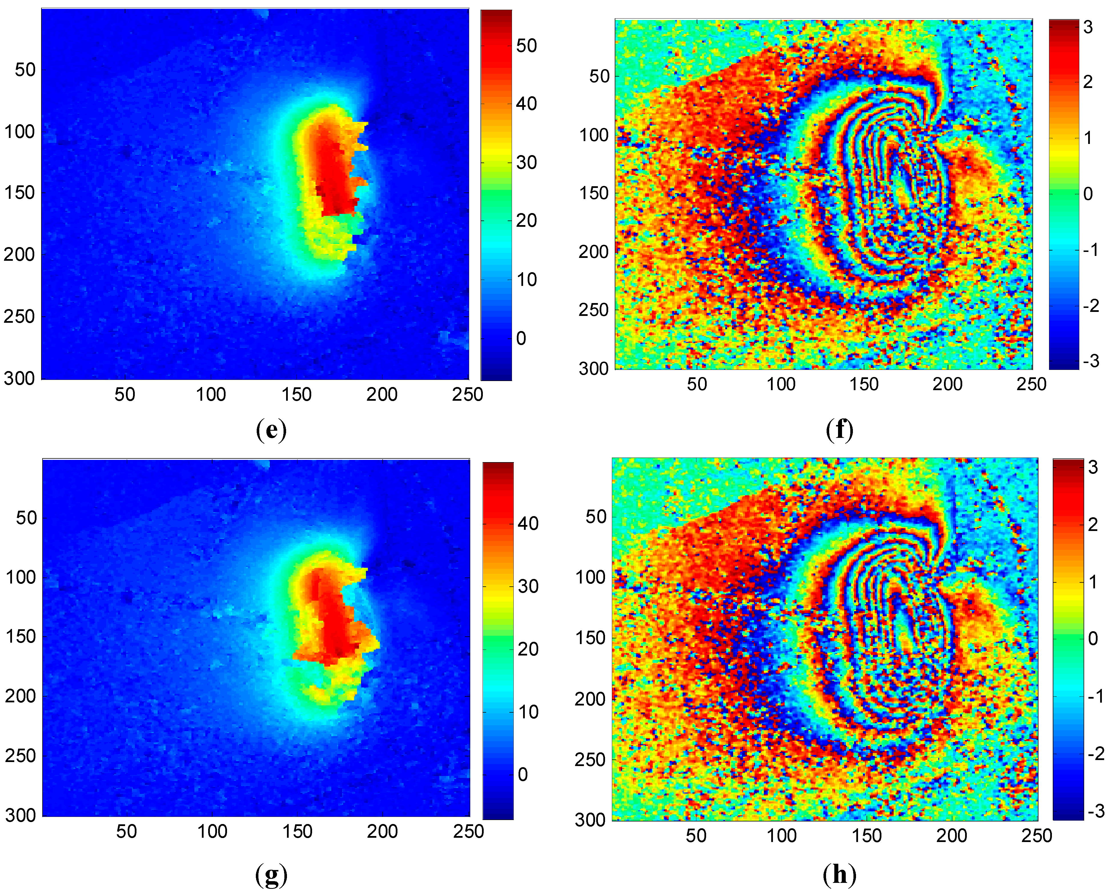
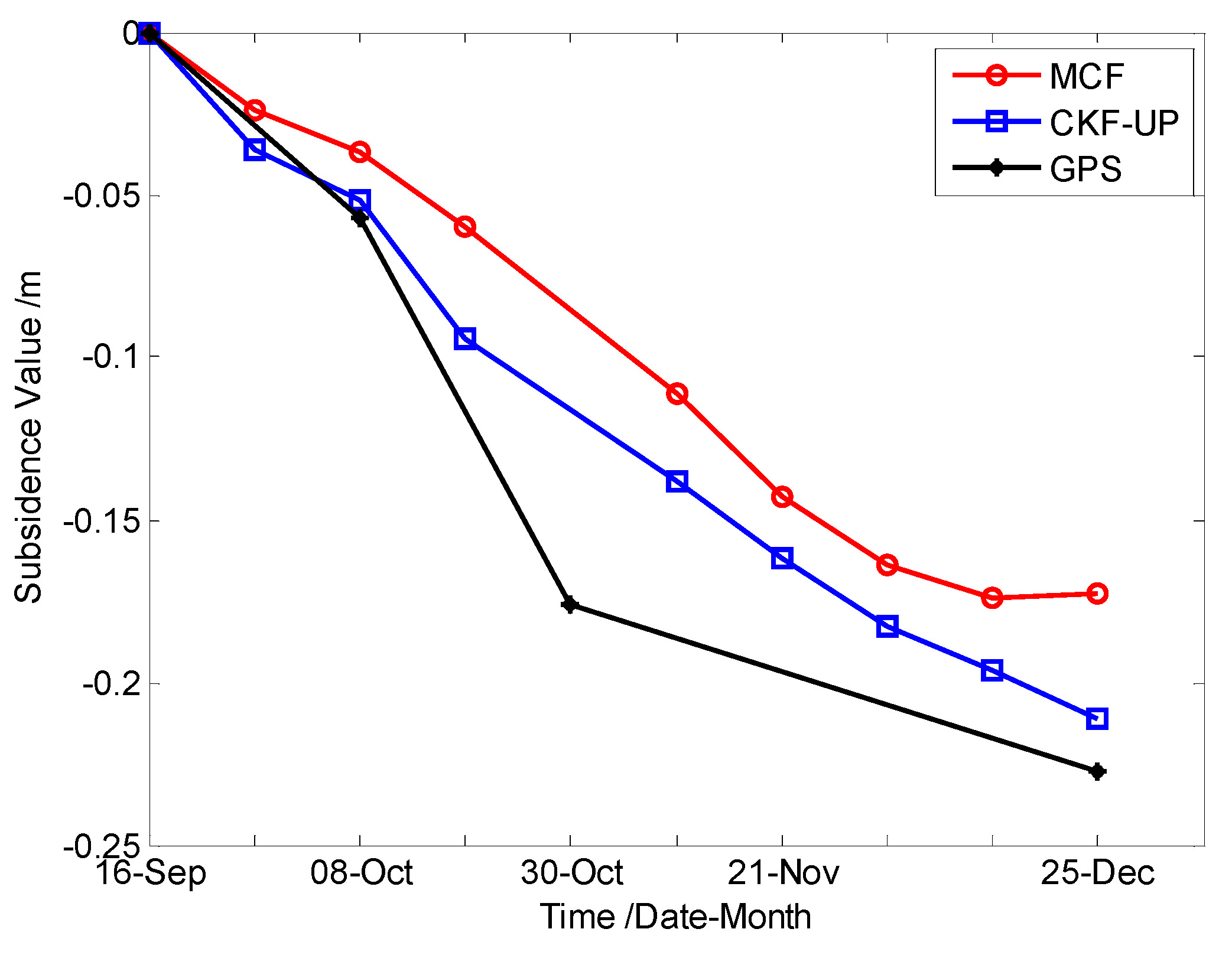
4.2.3. Case 3
| ID | SAR Data | Pre-Filtering + MCF | CKFPU | GPS Result | |||
|---|---|---|---|---|---|---|---|
| Master | Slave | SSV/m | ASV/m | SSV/m | ASV/m | ASV/m | |
| 1 | 16 September 2012 | 27 September 2012 | −0.024 | −0.024 | −0.036 | −0.036 | —— |
| 2 | 27 September 2012 | 8 October 2012 | −0.013 | −0.037 | −0.016 | −0.052 | −0.057 |
| 3 | 8 October 2012 | 19 October 2012 | −0.023 | −0.060 | −0.042 | −0.094 | —— |
| 4 | 19 October 2012 | 10 November 2012 | −0.051 | −0.111 | −0.044 | −0.138 | −0.176 |
| 5 | 10 November 2012 | 21 November 2012 | −0.032 | −0.143 | −0.024 | −0.162 | —— |
| 6 | 21 November 2012 | 2 December 2012 | −0.020 | −0.164 | −0.021 | −0.183 | —— |
| 7 | 2 December 2012 | 13 December 2012 | −0.011 | −0.174 | −0.013 | −0.196 | —— |
| 8 | 13 December 2012 | 24 December 2012 | 0.002 | −0.173 | −0.005 | −0.201 | −0.227 |
5. Conclusions
Acknowledgments
Author Contributions
Conflicts of Interest
References
- Wegmüller, U.; Werner, C.; Strozzi, T.; Wiesmann, A. Monitoring mining induced surface deformation. In Proceedings of the 2004 IEEE Geoscience and Remote Sensing Symposium, IGARSS’04, Anchorage, AK, USA, 20–24 September 2004; Volume 3, pp. 1933–1935.
- Liu, D.; Shao, Y.; Liu, Z.; Riedel, B.; Sowter, A.; Niemeier, W.; Bian, Z. Evaluation of InSAR and TomoSAR for monitoring deformations caused by mining in a mountainous area with high resolution satellite-based SAR. Remote Sens. 2014, 6, 1476–1495. [Google Scholar] [CrossRef]
- Liu, Z.; Bian, Z.; Lei, S.; Liu, D.; Sowter, A. Evaluation of PS-DInSAR technology for subsidence monitoring caused by repeated mining in mountainous area. Trans. Nonferrous Met. Soc. China 2014, 24, 3309–3315. [Google Scholar] [CrossRef]
- Ghiglia, D.C.; Pritt, M.D. Two-dimentional Phase Unwrapping. In Theory, Algorithms and Software; Wiley: New York, NY, USA, 1998. [Google Scholar]
- Gens, R. Two-dimensional phase unwrapping for radar interferometry: Developments and new challenges. Int. J. Remote Sens. 2003, 24, 703–710. [Google Scholar] [CrossRef]
- Goldstein, R.M.; Zebker, H.A.; Werner, C.L. Satellite radar interferometry: Two-dimensional phase unwrapping. Radio Sci. 1988, 23, 713–720. [Google Scholar] [CrossRef]
- Xu, W.; Cumming, I. A region-growing algorithm for InSAR phase unwrapping. IEEE Trans. Geosci. Remote Sens. 1999, 37, 124–133. [Google Scholar] [CrossRef]
- Flynn, T.J. Two dimensional phase unwrapping with minimum weighted discontinuity. J. Opt. Soc. Am. 1997, 14, 2692–2710. [Google Scholar] [CrossRef]
- Costantini, M. A novel phase unwrapping method based on network programming. IEEE Trans. Geosci. Remote Sens. 1998, 36, 813–821. [Google Scholar] [CrossRef]
- Ghiglia, D.; Romero, L. Robust two-dimensional weighted and unweighted phase unwrapping that uses fast transforms and iterative methods. J. Opt. Soc. Am. A 1994, 11, 107–117. [Google Scholar] [CrossRef]
- Lee, J.-S.; Papathanassiou, K.P.; Ainsworth, T.L.; Grunes, M.R.; Reigbe, A. A new technique for noise filtering of SAR interferometric phase images. IEEE Trans. Geosci. Remote Sens. 1998, 36, 1456–1465. [Google Scholar]
- Wu, N.; Feng, D.-Z.; Li, J. A locally adaptive filter of interferometric phase images. IEEE Trans. Geosci. Remote Sens. Lett. 2006, 3, 73–77. [Google Scholar] [CrossRef]
- Yu, Q.; Yang, X.; Fu, S.; Liu, X.; Sun, X. An adaptive contoured window filter for interferometric synthetic aperture radar. IEEE Trans. Geosci. Remote Sens. Lett. 2007, 4, 23–26. [Google Scholar] [CrossRef]
- Suksmono, A.B.; Hirose, A. Adaptive noise reduction of InSAR images based on a complex-valued MRF model and its applications to phase unwrapping problem. IEEE Trans. Geosci. Remote Sens. 2002, 40, 699–709. [Google Scholar] [CrossRef]
- Kim, M.; Griffiths, H. Phase unwrapping of multibaseline interferometry using Kalman filtering. In Proceedings of the Seventh International Conference on Image Processing and Its Applications, Manchester, UK, 13–15 July 1999; pp. 813–817.
- Loffeld, O.; Nies, H.; Knedlik, S.; Wang, Y. Phase unwrapping for SAR interferometry—A data fusion approach by kalman filtering. IEEE Trans. Geosci. Remote Sens. 2008, 46, 47–58. [Google Scholar] [CrossRef]
- Nies, H.; Loffeld, O.; Wang, R. Phase unwrapping using 2d-kalman filter—Potential and limitations. In Proceedings of the IEEE International Geoscience and Remote Sensing Symposium, Boston, MA, USA, 7–11 July 2008; pp. 1213–1216.
- Osmanoǧlu, B.; Wdowinski, S.; Dixon, T.H.; Biggs, J. InSAR phase unwrapping based on extended Kalman filtering. IEEE Trans. Geosci. Remote Sens. 2009, 47, 1197–1202. [Google Scholar]
- Martinez-Espla, J.; Martinez-Marin, T.; Lopez-Sanchez, J. A Particle Filter Approach for InSAR Phase Filtering and Unwrapping. IEEE Trans. Geosci. Remote Sens. 2009, 47, 1197–1211. [Google Scholar] [CrossRef]
- Osmanoǧlu, B.; Dixon, T.H.; Wdowinski, S. Three-Dimensional Phase Unwrapping for Satellite radar interferometry, I DEM generation. IEEE Trans. Geosci. Remote Sens. 2014, 52, 1059–1075. [Google Scholar] [CrossRef]
- Xie, X.; Pi, Y. Phase noise filtering and phase unwrapping method based on unscented Kalman filter. J. Syst. Eng. Electron. 2011, 22, 365–372. [Google Scholar]
- Xie, X.; Pi, Y.; Peng, B. Phase unwrapping: An unscented particle filtering approach. Acta Electron. Sin. 2011, 39, 705–709. (In Chinese) [Google Scholar]
- Liu, W.; Zhang, Q. New Strong Tracking Filter Based on Cubature Kalman Filter. J. Syst. Simul. 2014, 26, 1102–1107. (In Chinese) [Google Scholar]
- Ienkaran, A.; Simon, H. Cubature kalman filters. IEEE Trans. Autom. Control 2009, 54, 1254–1269. [Google Scholar]
- Ienkaran, A. Cubature Kalman Filtering: Theory & Applications. Ph.D. Thesis, McMaster University, Hamilton, ON, Canada, 2009. [Google Scholar]
- Jia, B.; Xin, M.; Cheng, Y. High-degree Cubature Kalman filter. Automatica 2013, 49, 510–518. [Google Scholar] [CrossRef]
- Spagnolini, U. 2-D phase unwrapping and instantaneous frequency estimation. IEEE Trans. Geosci. Remote Sens. 1995, 33, 579–589. [Google Scholar] [CrossRef]
- Trouve, E.; Nicolas, J.M.; Maitre, H. Improving phase unwrapping techniques by the use of local frequency estimates. IEEE Trans. Geosci. Remote Sens. 1998, 36, 1963–1965. [Google Scholar] [CrossRef]
- Jiang, M.; Li, Z.; Ding, X.; Zhu, J.; Feng, G. Modeling minimum and maximum detectable deformation gradients of interferometric SAR measurements. Int. J. Appl. Earth Obs. Geoinf. 2011, 13, 766–777. [Google Scholar] [CrossRef]
- Osmanoǧlu, B.; Dixon, T.H.; Wdowinski, S.; Cabral-Cano, E. On the importance of Path for Phase Unwrapping in Synthetic Aperture Radar Interferometry. Appl. Opt. 2011, 50, 3205–3220. [Google Scholar] [CrossRef] [PubMed]
- Just, D.; Bamler, R. Phase statistics of interferograms with application to synthetic aperture radar. Appl. Opt. 1994, 33, 4361–4368. [Google Scholar] [CrossRef] [PubMed]
© 2015 by the authors; licensee MDPI, Basel, Switzerland. This article is an open access article distributed under the terms and conditions of the Creative Commons Attribution license (http://creativecommons.org/licenses/by/4.0/).
Share and Cite
Liu, W.; Bian, Z.; Liu, Z.; Zhang, Q. Evaluation of a Cubature Kalman Filtering-Based Phase Unwrapping Method for Differential Interferograms with High Noise in Coal Mining Areas. Sensors 2015, 15, 16336-16357. https://doi.org/10.3390/s150716336
Liu W, Bian Z, Liu Z, Zhang Q. Evaluation of a Cubature Kalman Filtering-Based Phase Unwrapping Method for Differential Interferograms with High Noise in Coal Mining Areas. Sensors. 2015; 15(7):16336-16357. https://doi.org/10.3390/s150716336
Chicago/Turabian StyleLiu, Wanli, Zhengfu Bian, Zhenguo Liu, and Qiuzhao Zhang. 2015. "Evaluation of a Cubature Kalman Filtering-Based Phase Unwrapping Method for Differential Interferograms with High Noise in Coal Mining Areas" Sensors 15, no. 7: 16336-16357. https://doi.org/10.3390/s150716336
APA StyleLiu, W., Bian, Z., Liu, Z., & Zhang, Q. (2015). Evaluation of a Cubature Kalman Filtering-Based Phase Unwrapping Method for Differential Interferograms with High Noise in Coal Mining Areas. Sensors, 15(7), 16336-16357. https://doi.org/10.3390/s150716336