
A Cross Structured Light Sensor and Stripe Segmentation Method for Visual Tracking of a Wall Climbing Robot


Abstract
:1. Introduction
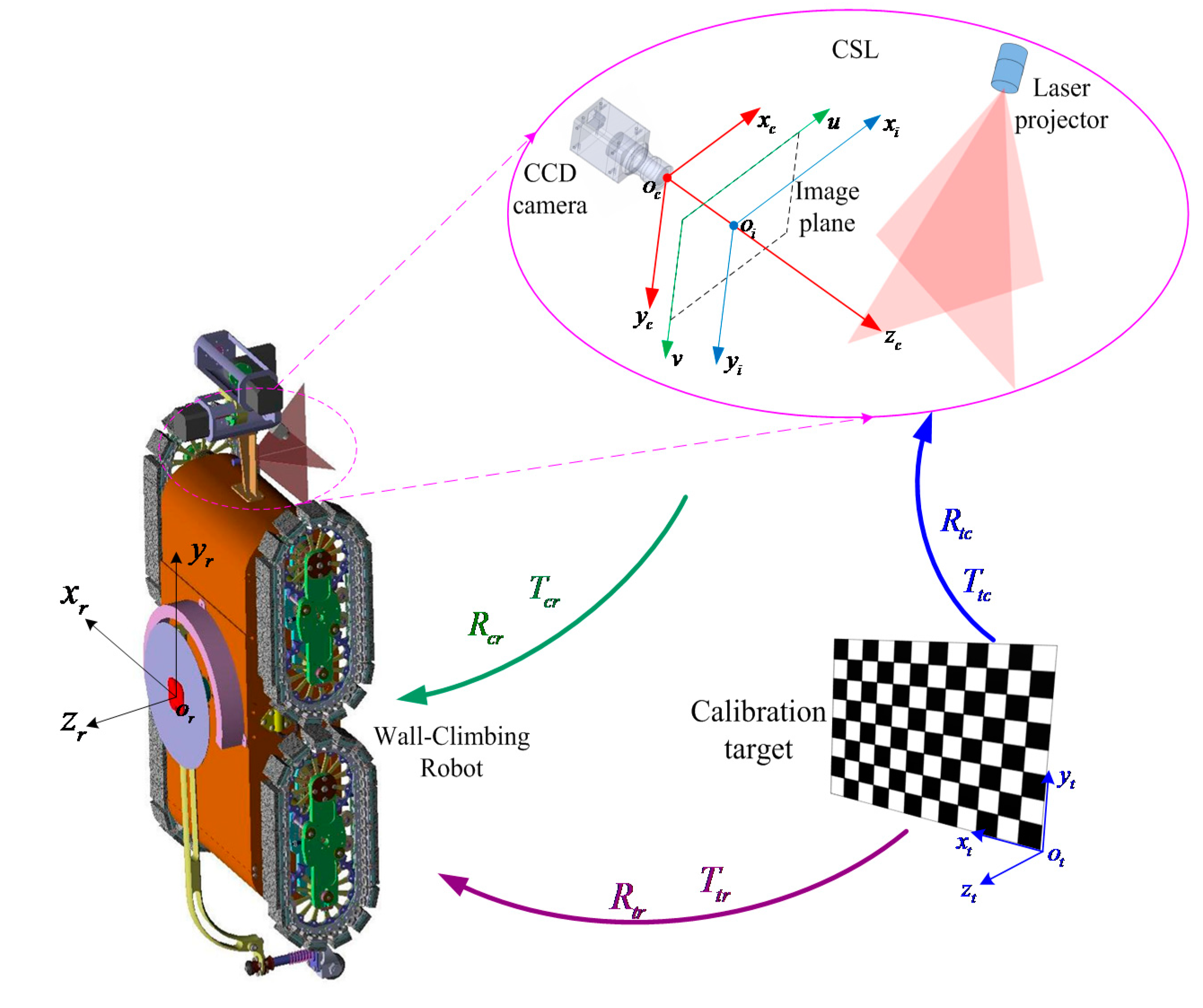
2. Cross Structured Light Sensor
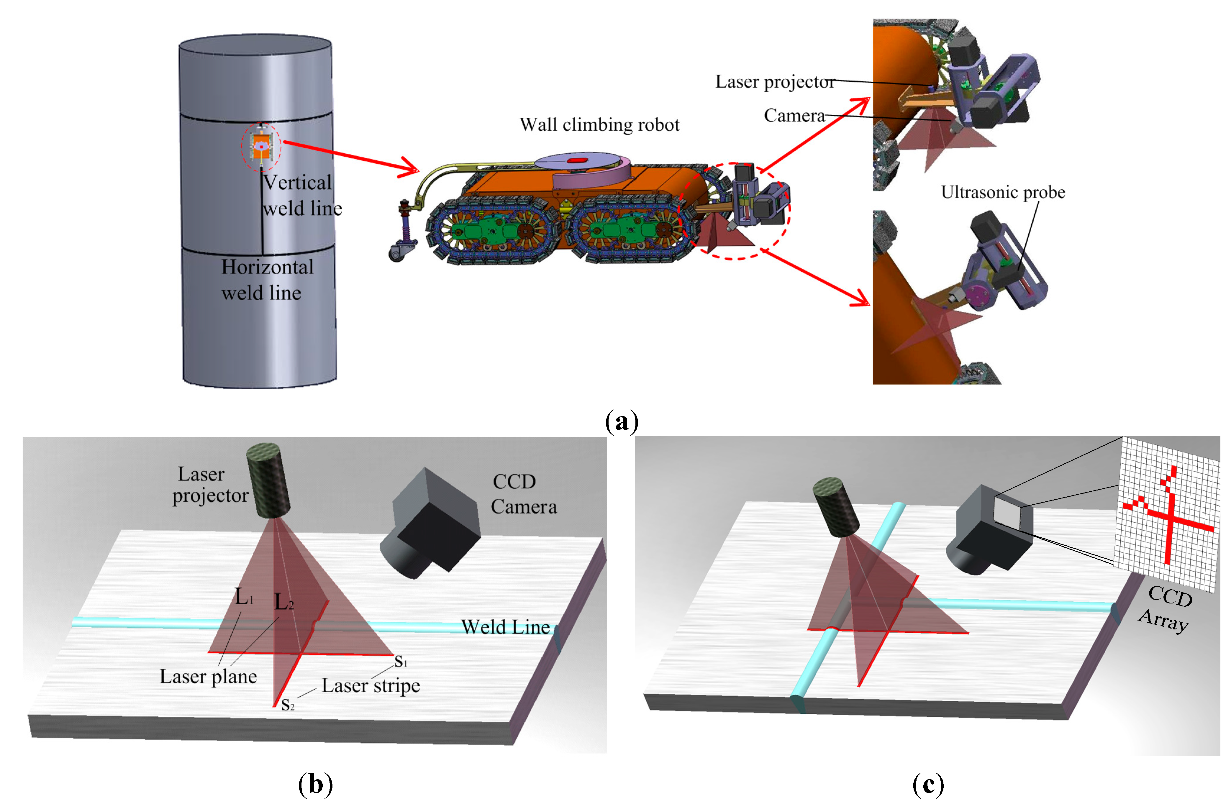
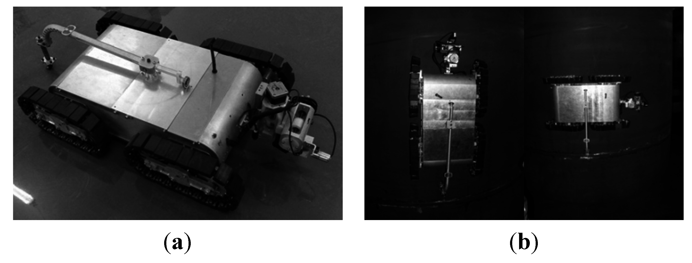
2.1. The Robot Platform

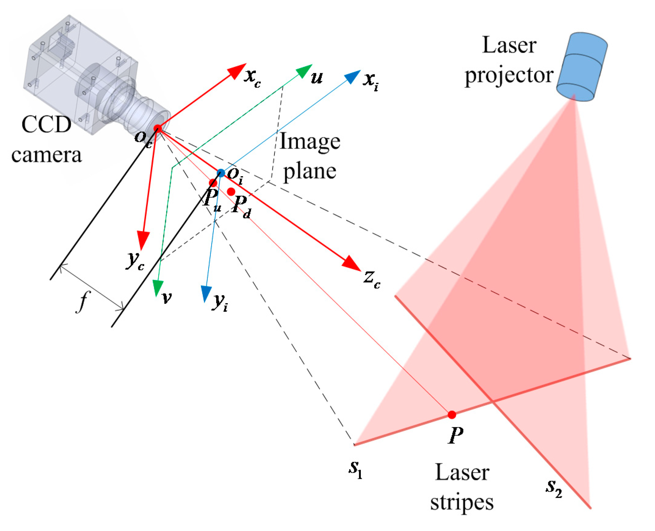
2.2. Model of CSL Sensor

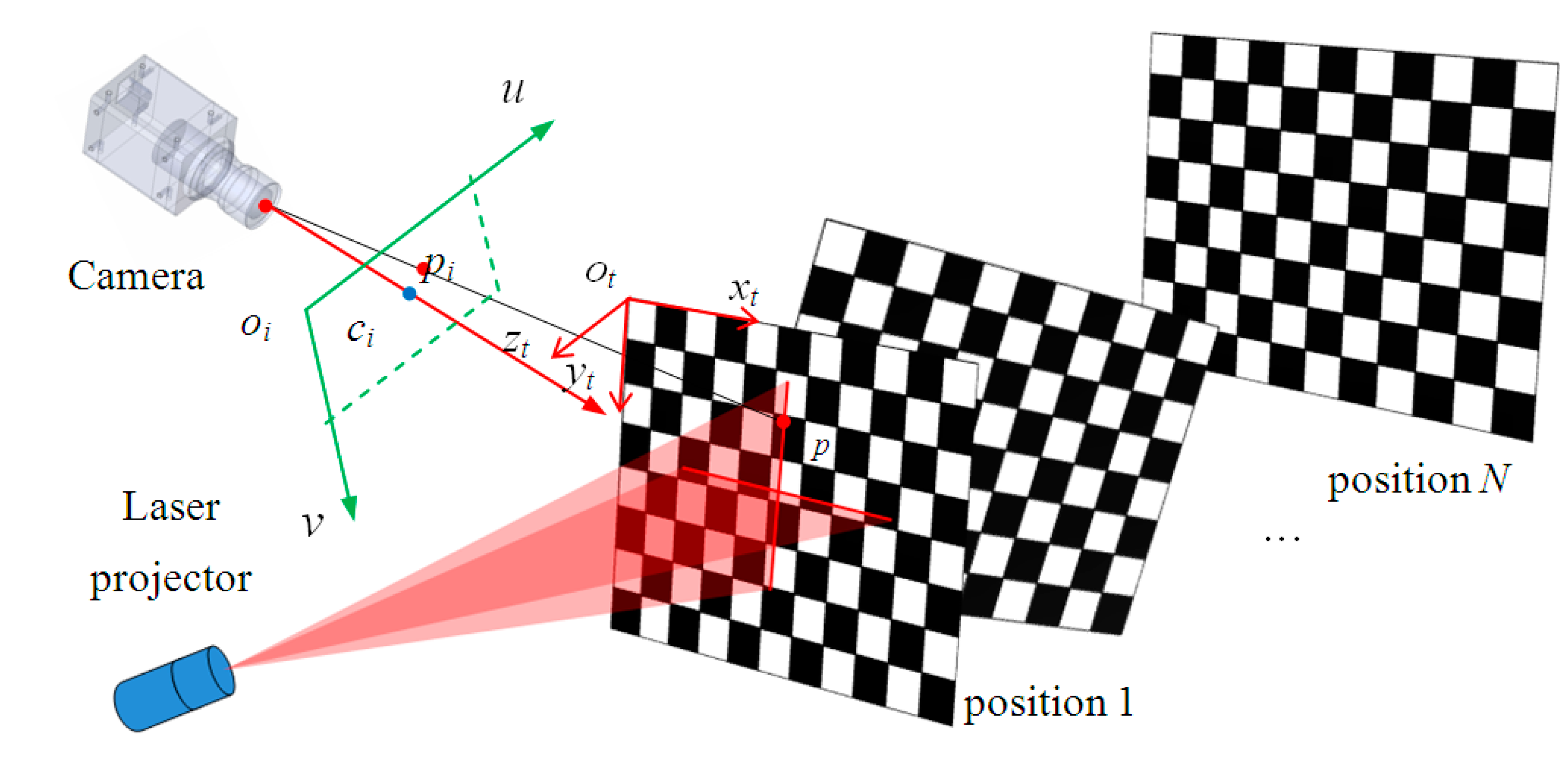
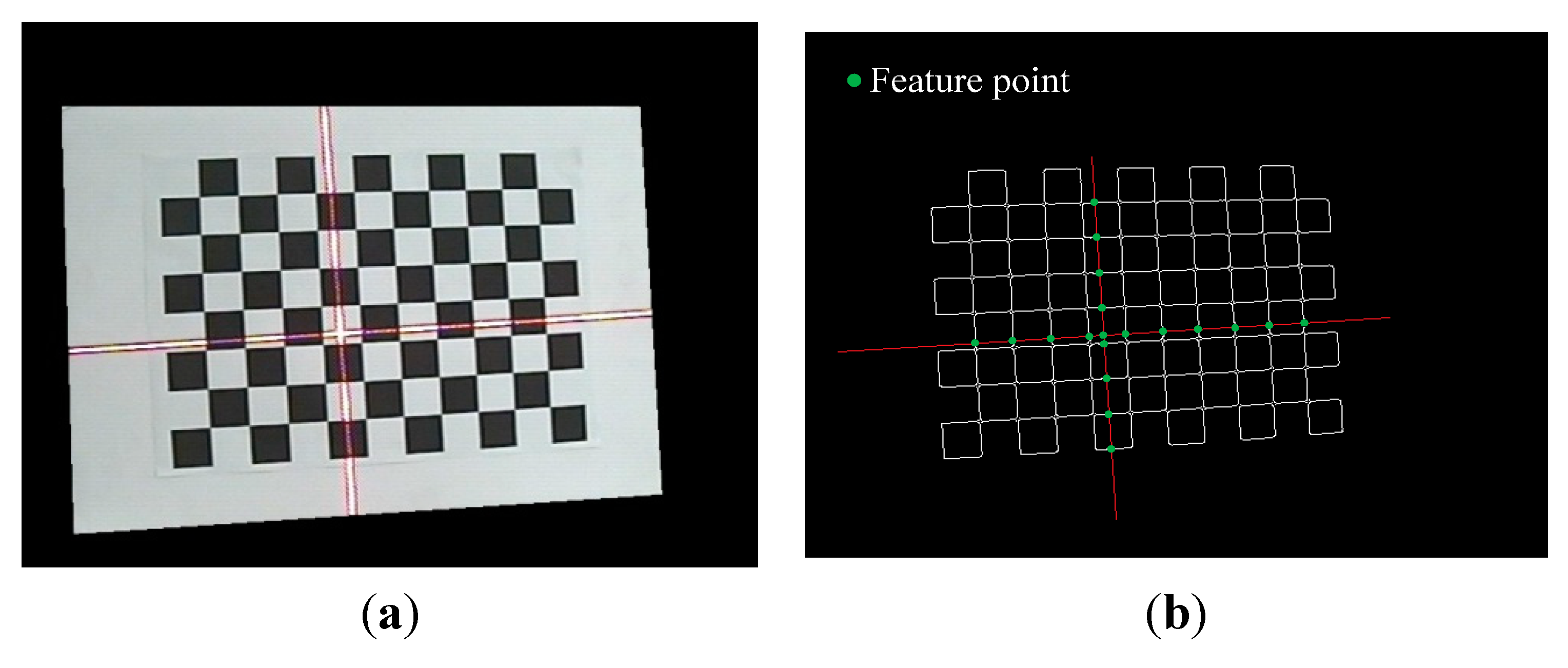
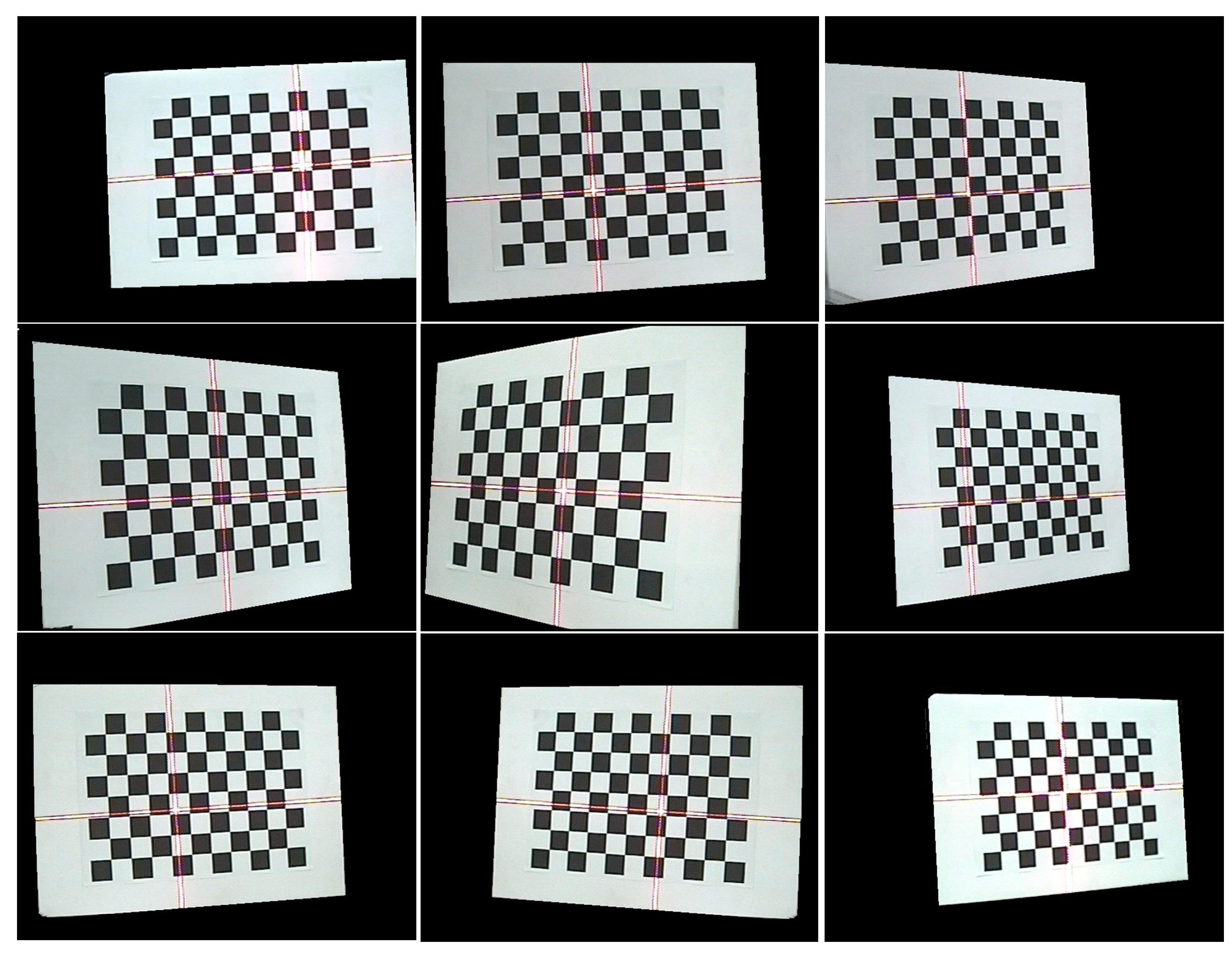
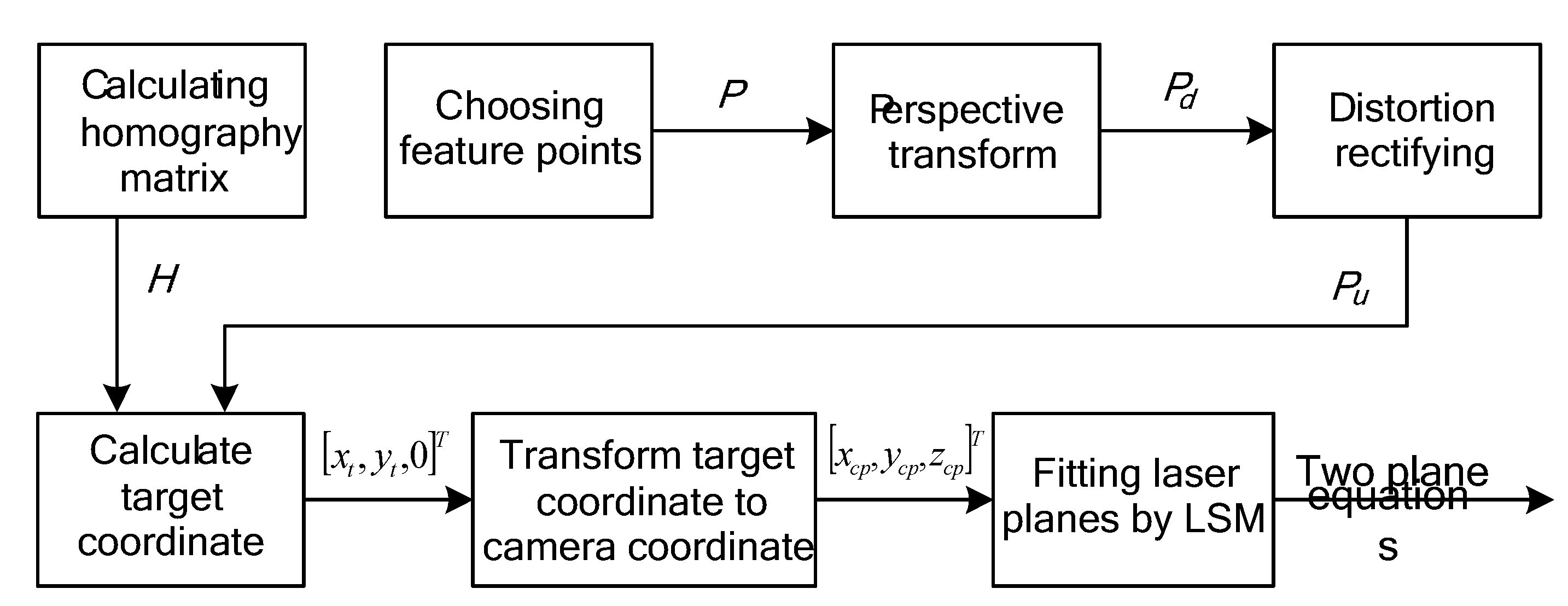
2.3. Calibration of CSL Sensor

| Category | Parameters | Physical Meaning |
|---|---|---|
| Camera intrinsic parameters | (fx, fy) | Focal length in the x, y direction |
| (u0, v0) | Principle point coordinates | |
| (k1, k2) | Radial distortion parameters | |
| (p1, p2) | Tangential distortion parameters | |
| Light plane equations | (a1, b1, c1) | Laser plane L1 equation coefficients |
| (a2, b2, c2) | Laser plane L2 equation coefficients | |
| ∠ l1ol2 | Angle between L1 and L2 | |
| Global parameters | Rcr | Rotation from oc-xcyczc to or-xryrzr |
| Tcr | Translation from oc-xcyczc to or-xryrzr |


3. Laser Stripe Segmentation and Centre Points Localization
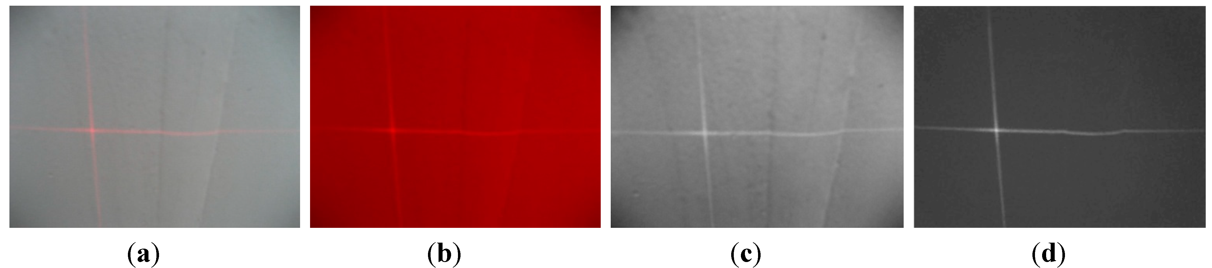
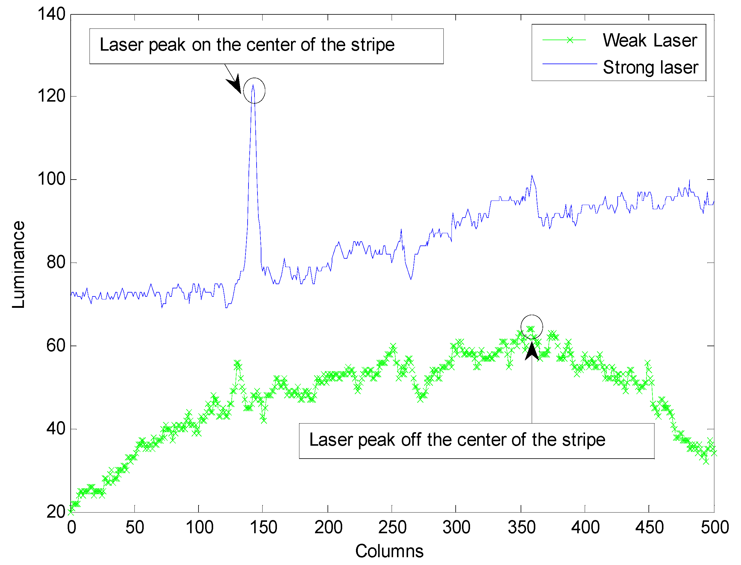
3.1. Preprocessing Based on Monochromatic Value Space
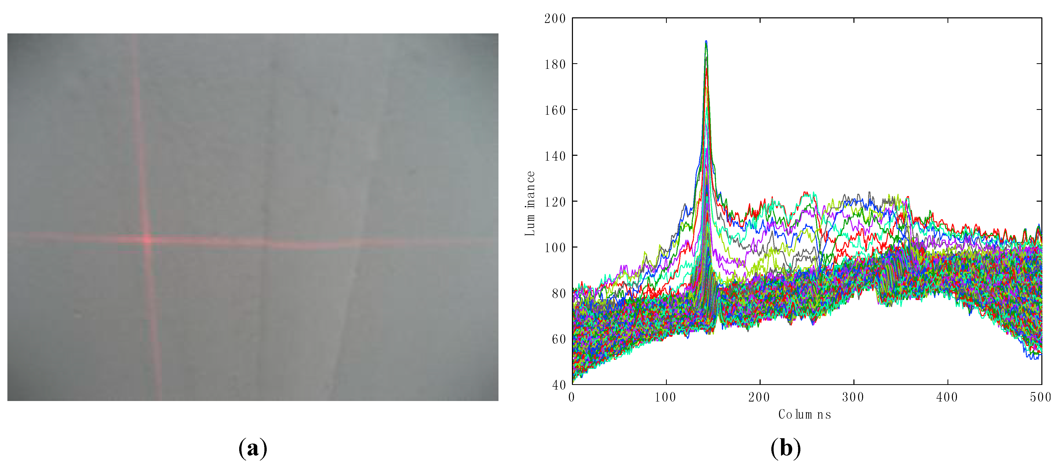
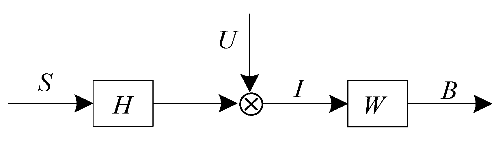
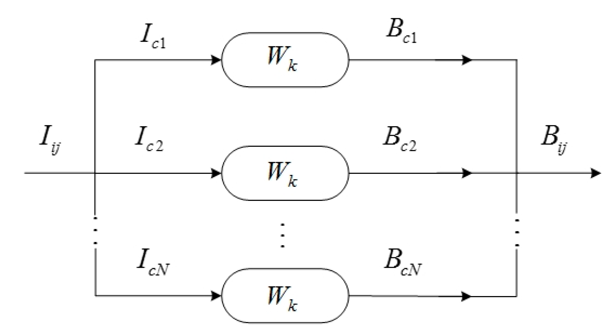
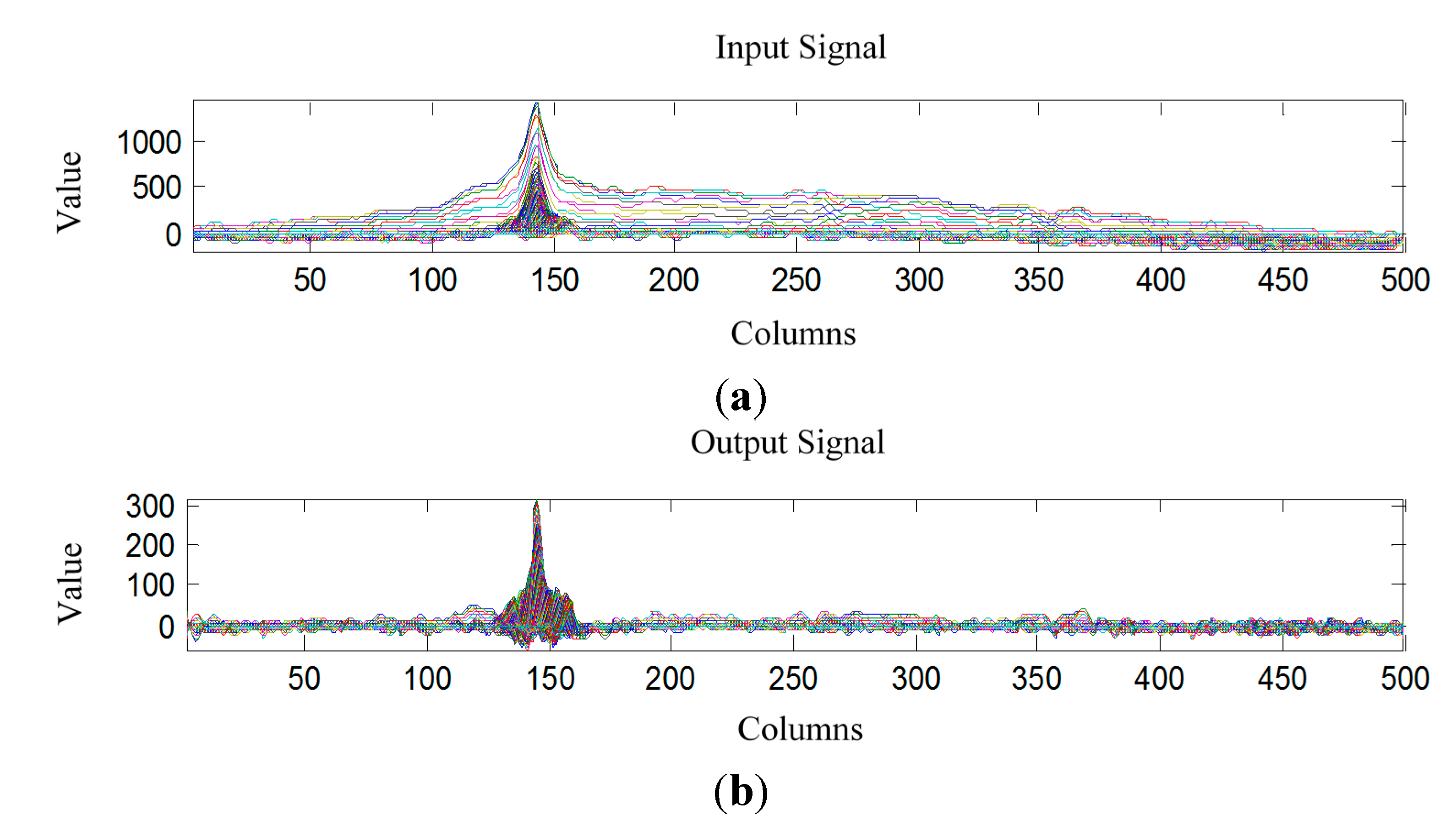
3.2. Stripe Segmentation Based on Minimum Entropy Deconvolution(MED)

- S denotes the laser stripe;
- H denotes the point spread function of the optical imaging system;
- U denotes a noise function;
- I denotes the acquired image;
- * denotes the 2D convolution operator;
- (i, j) is discrete spatial coordinates;
- W denotes the finite impulse response (FIR) filter, W = 0 if i < 1or j < 1, and W*H = δi-Δi,j-Δj, where δij is the Krönecker delta (discrete impulse signal) [37], and Δi, Δj are the phase delay;
- B denotes the recovered image.

| Step | Algorithm |
|---|---|
| 1 | Initializing the adaptive FIR filter, and setting Wk = [11...1...11]/, K = 0. |
| 2 | Computing the output signal Bij according to Equation (11). |
| 3 | Inputting Bij to Equations (22)–(24), Wk is obtained. |
| 4 | Inputting Bij to Equation (19) to compute kurtosis K and . |
| 5 | Repeating step 2 and 3 to make sure that a specified number of iterations is achieved and that the change in K between iterations is less than a specified small value. |

3.3. Centre Points Localization of Laser Stripe

4. Results and Discussion
| Device | Parameters |
|---|---|
| Camera | CCD: SONY: 1/4 inch |
| Resolution: 640 × 480 pixels | |
| Pixel size: 5.6 μm × 5.6 μm | |
| Frame rate: 20 fps | |
| Focal length: 8 mm | |
| Field of view: 43.7° | |
| Laser projector | Size: 9 × 23 mm |
| Wavelength: 700 nm | |
| Operating voltage: DC 5 V | |
| Operating current: 20–50 mA | |
| Output power: 250 mW | |
| Fan angle: 60° |
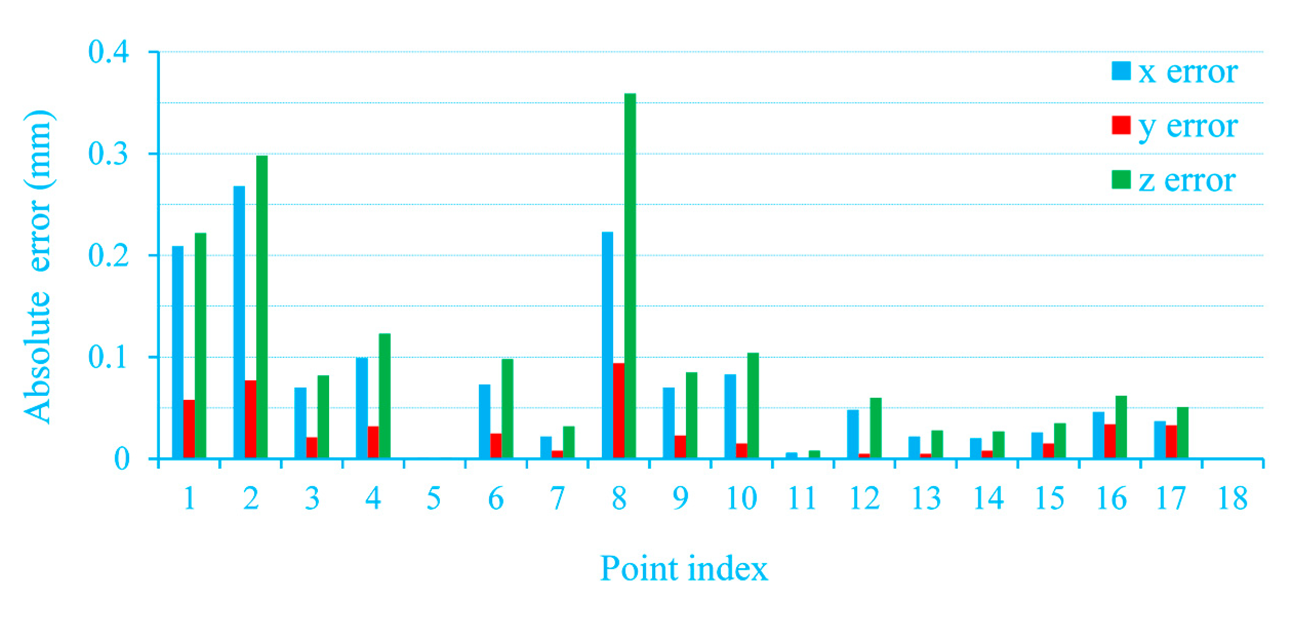
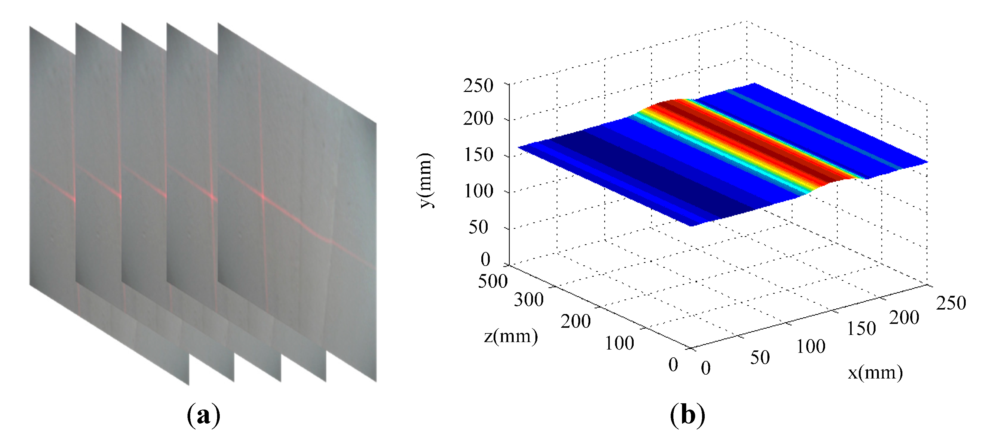
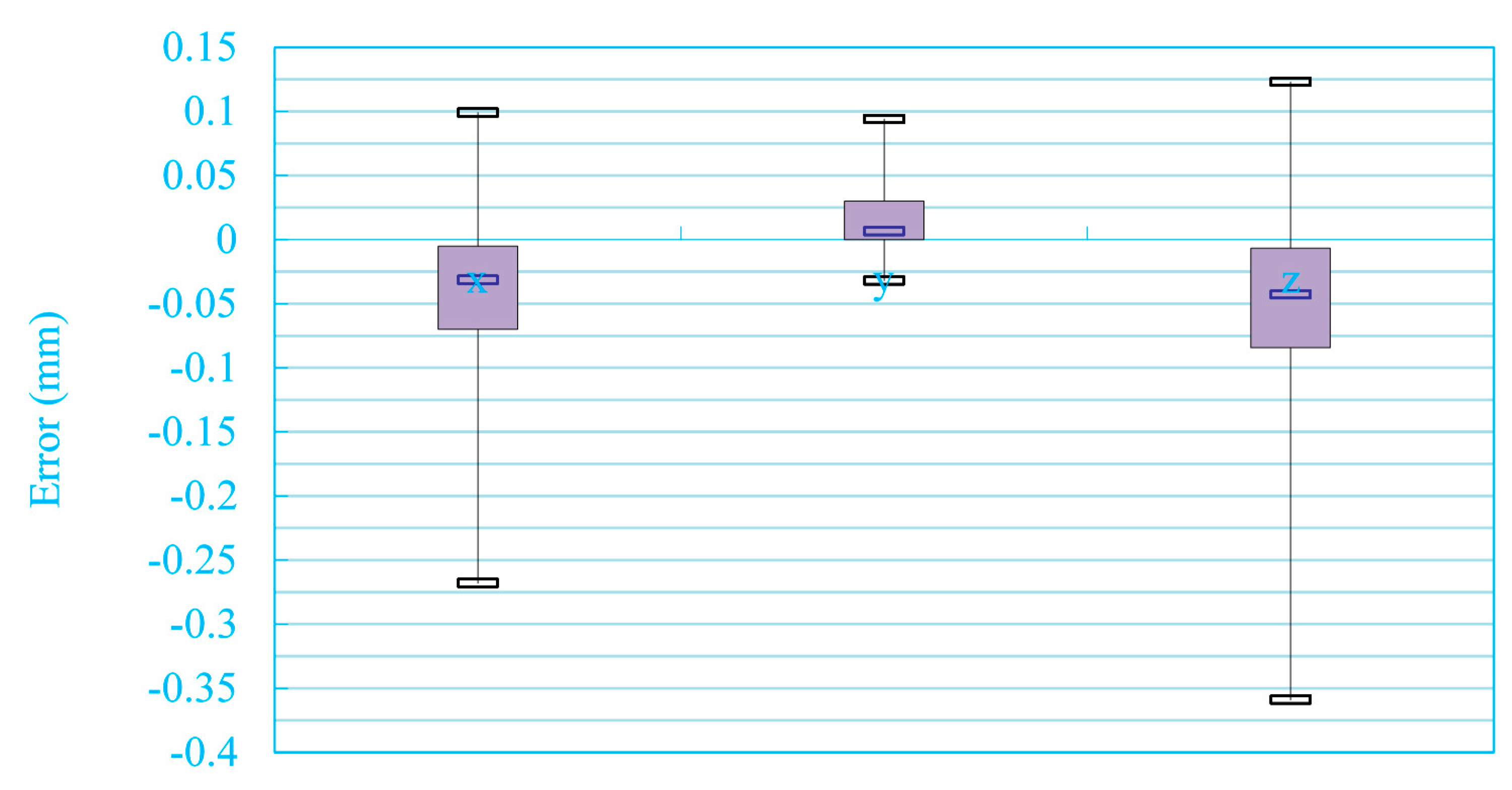
4.1. CSL Sensor Calibration

| Category | Parameters | Values |
|---|---|---|
| Camera intrinsic parameters | (fx, fy) | (922.4350, 917.3560) |
| (u0, v0) | (329.1680, 2705660) | |
| (k1, k2) | (−291.459 × 10⁻³, 157.027 × 10⁻³) | |
| (p1, p2) | (−0.1354 × 10⁻³, −0.2682 × 10⁻³) | |
| Light plane equations | (a1, b1, c1) | (−0.18 × 10⁻³, 1.86 × 10⁻³, 1.39 × 10⁻³) |
| (a2, b2, c2) | (−90.11 × 10⁻³, 2.463 × 10⁻³, 8.935 × 10⁻³) | |
| ∠l1ol2 | 89.9981° | |
| Global parameters | Rcr | |
| Tcr |
| Image Coordinates | Standard Value | Measured Value | Errors of Coordinates | ||||||
|---|---|---|---|---|---|---|---|---|---|
| (u,v)/(pixels) | x (mm) | y (mm) | z (mm) | x (mm) | y (mm) | z (mm) | Δx (mm) | Δy (mm) | Δz (mm) |
| 434.812, 216.242 | 224.751 | −61.644 | 237.893 | 224.542 | −61.586 | 237.671 | −0.209 | 0.058 | −0.222 |
| 521.702, 339.656 | 208.124 | −60.198 | 231.686 | 207.856 | −60.121 | 231.388 | −0.268 | 0.077 | −0.298 |
| 520.861, 304.699 | 191.494 | −58.802 | 225.479 | 191.424 | −58.781 | 225.397 | −0.070 | 0.021 | −0.082 |
| 519.817, 272.006 | 174.863 | −57.407 | 219.272 | 174.962 | −57.439 | 219.395 | 0.099 | −0.032 | 0.123 |
| 518.237, 238.050 | 166.850 | −56.695 | 216.280 | 166.851 | −56.695 | 216.281 | 0.001 | 0 | 0.001 |
| 516.309, 220.555 | 158.236 | −55.971 | 213.065 | 158.309 | −55.996 | 213.163 | 0.073 | −0.025 | 0.098 |
| 515.171, 204.063 | 141.610 | −54.515 | 206.858 | 141.588 | −54.507 | 206.826 | −0.022 | 0.008 | −0.032 |
| 512.486, 170.342 | 124.986 | −53.019 | 200.650 | 124.763 | −52.925 | 200.291 | −0.223 | 0.094 | −0.359 |
| 508.894, 138.080 | 177.332 | 57.495 | 216.540 | 177.262 | 57.472 | 216.455 | −0.070 | −0.023 | −0.085 |
| 577.181, 225.223 | 175.097 | 32.586 | 216.503 | 175.014 | 32.571 | 216.399 | −0.083 | −0.015 | −0.104 |
| 565.821, 224.684 | 172.689 | 7.687 | 216.400 | 172.695 | 7.687 | 216.408 | 0.006 | 0 | 0.008 |
| 554.325, 223.663 | 170.521 | −17.226 | 216.388 | 170.473 | −17.221 | 216.328 | −0.048 | 0.005 | −0.060 |
| 539.553, 223.101 | 168.219 | −42.131 | 216.325 | 168.197 | −42.126 | 216.297 | −0.022 | 0.005 | −0.028 |
| 525.946, 222.546 | 165.957 | −67.039 | 216.278 | 165.937 | −67.031 | 216.251 | −0.02 | 0.008 | −0.027 |
| 510.778, 220.525 | 163.709 | −91.947 | 216.235 | 163.683 | −91.932 | 216.200 | −0.026 | 0.015 | −0.035 |
| 494.025, 219.462 | 161.487 | −116.857 | 216.202 | 161.441 | −116.823 | 216.14 | −0.046 | 0.034 | −0.062 |
| 477.062, 218.398 | 159.212 | −141.763 | 216.150 | 159.175 | −141.730 | 216.099 | −0.037 | 0.033 | −0.051 |
| 457.027, 217.322 | 156.884 | -166.667 | 216.078 | 156.884 | −166.667 | 216.078 | 0 | 0 | 0 |
| RMS errors (mm) | -- | -- | -- | -- | -- | -- | 0.094 | 0.034 | 0.120 |

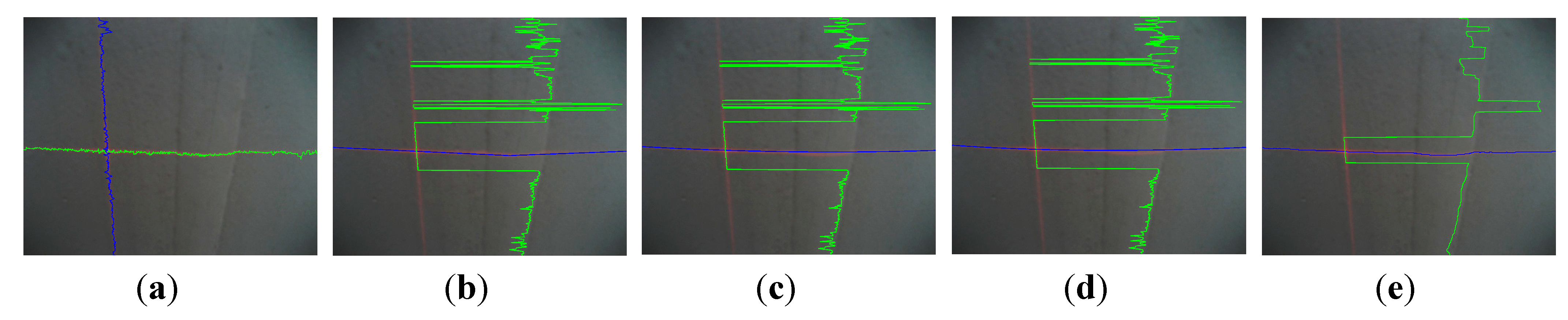
4.2. Accuracy and Speed of Stripe Segmentation

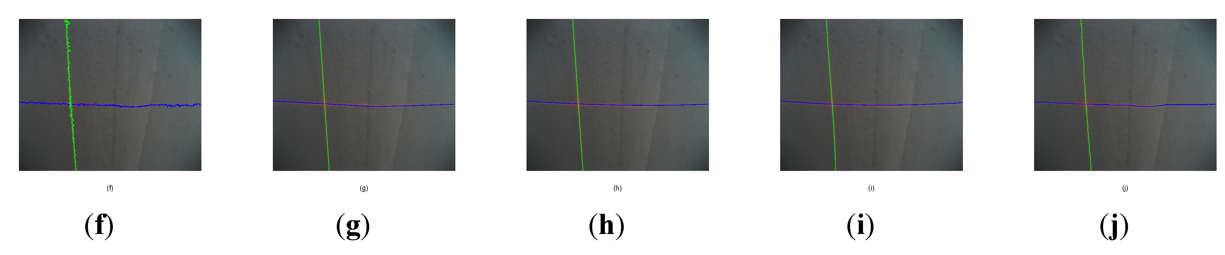
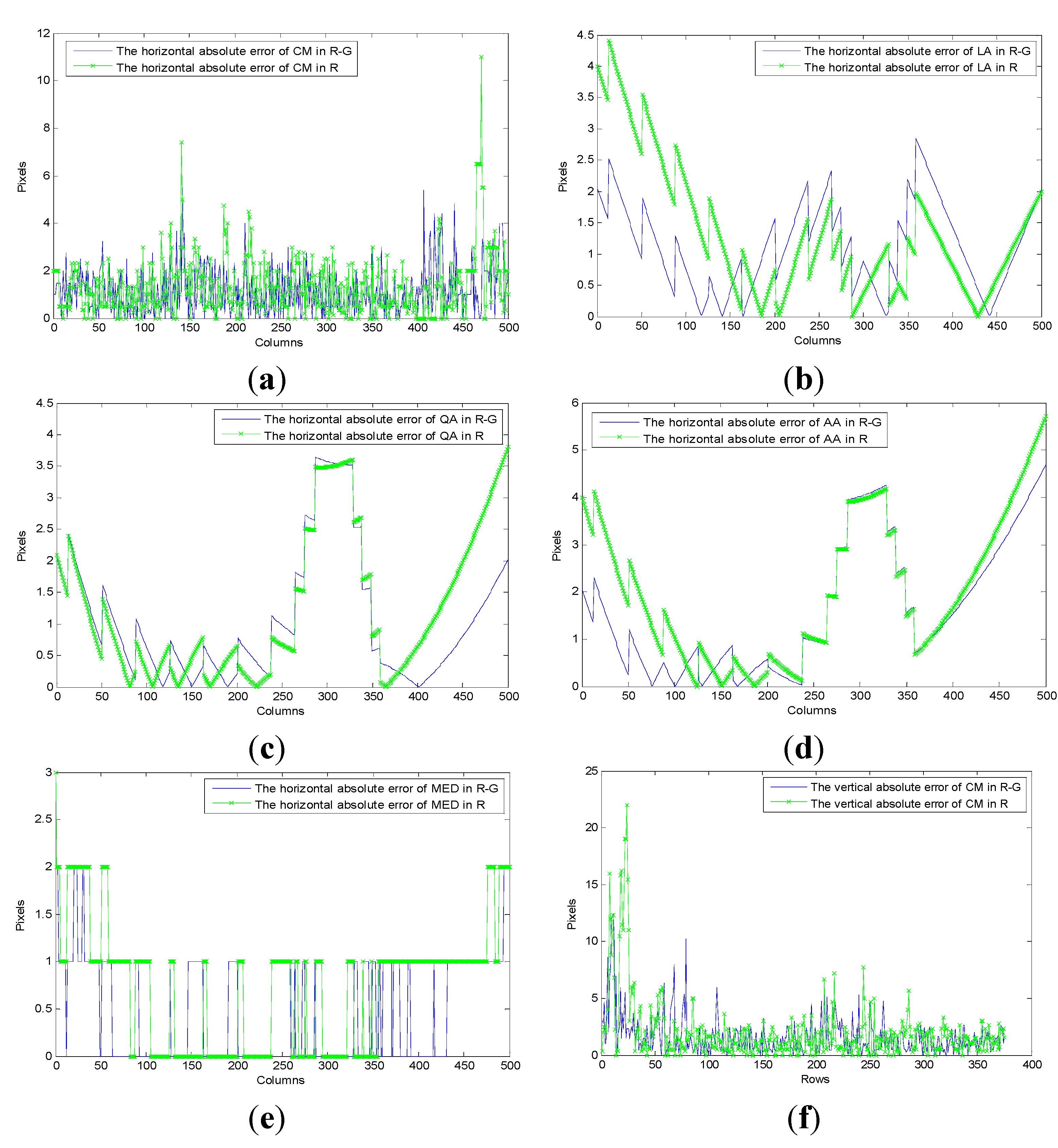

| Laser Stripe | Color Space | Method | CM | LA | QA | AA | MED | |
|---|---|---|---|---|---|---|---|---|
| Index | ||||||||
| Horizontal Laser stripe | R | Average error (mm) | 0.432 | 0.667 | 0.271 | 0.311 | 0.231 | |
| Running time (ms) | 18.3 | 320.2 | 168.1 | 130.3 | 22.3 | |||
| R-G | Average error (mm) | 0.330 | 0.416 | 0.267 | 0.291 | 0.231 | ||
| Running time (ms) | 17.9 | 314.0 | 167.6 | 196.6 | 20.9 | |||
| Vertical Laser stripe | R | Average error (mm) | 1.001 | 66.710 | 73.334 | 70.350 | 71.050 | |
| Running time (ms) | 18.8 | ∞ | ∞ | ∞ | 20.6 | |||
| R-G | Average error (mm) | 0.700 | 0.431 | 0.295 | 0.327 | 0.235 | ||
| Running time (ms) | 17.6 | 120.2 | 147.2 | 166.6 | 19.9 | |||
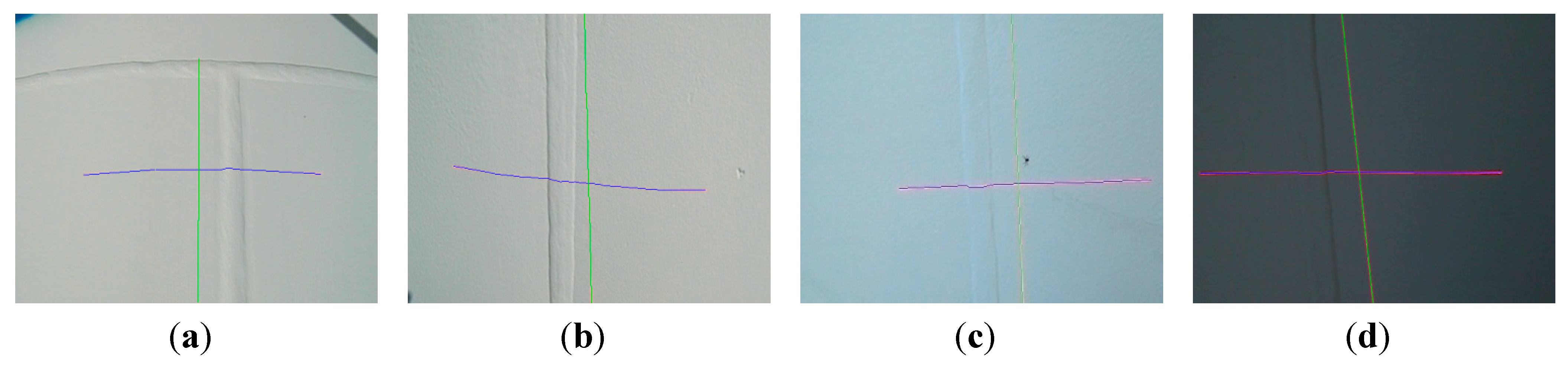
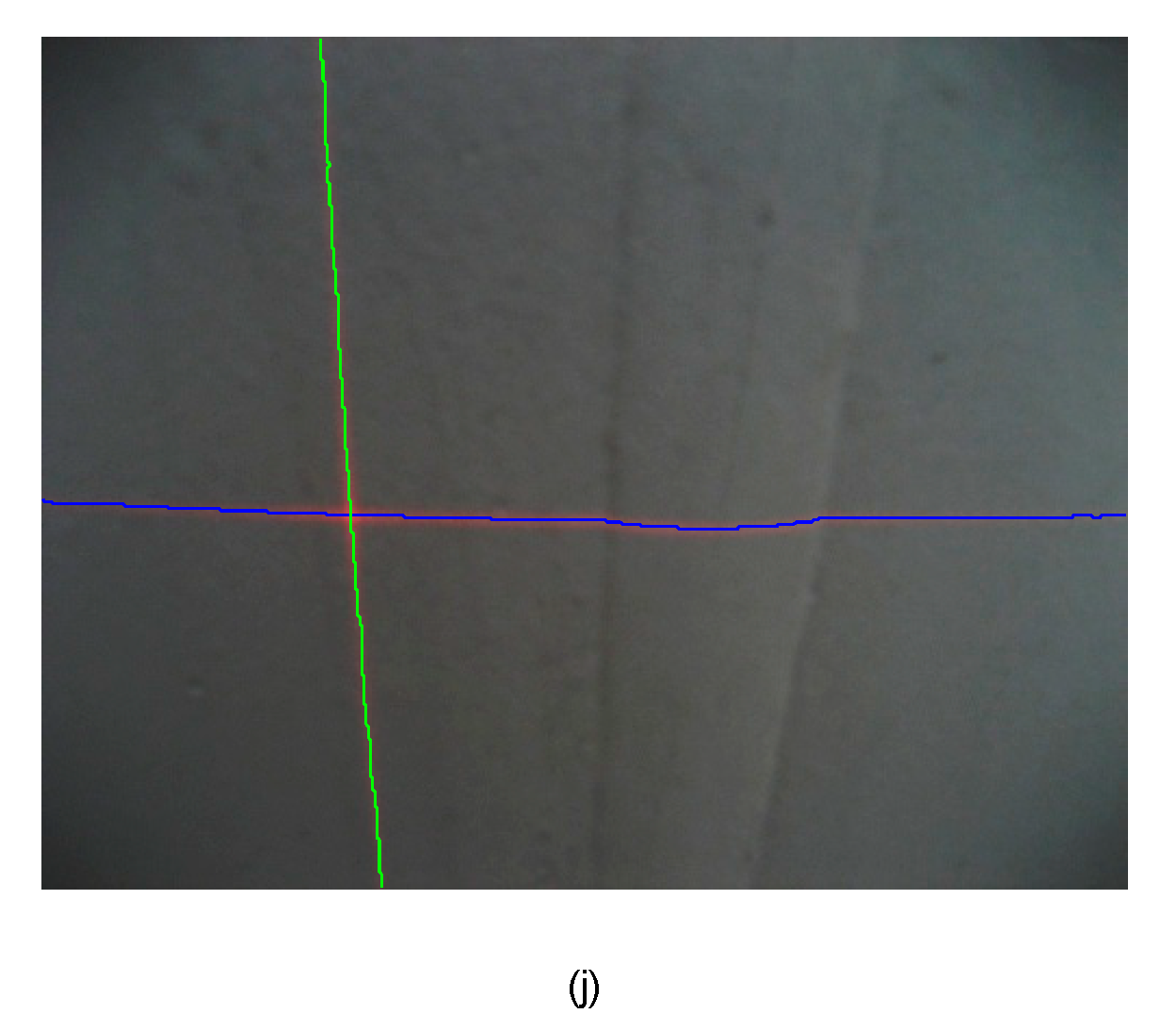
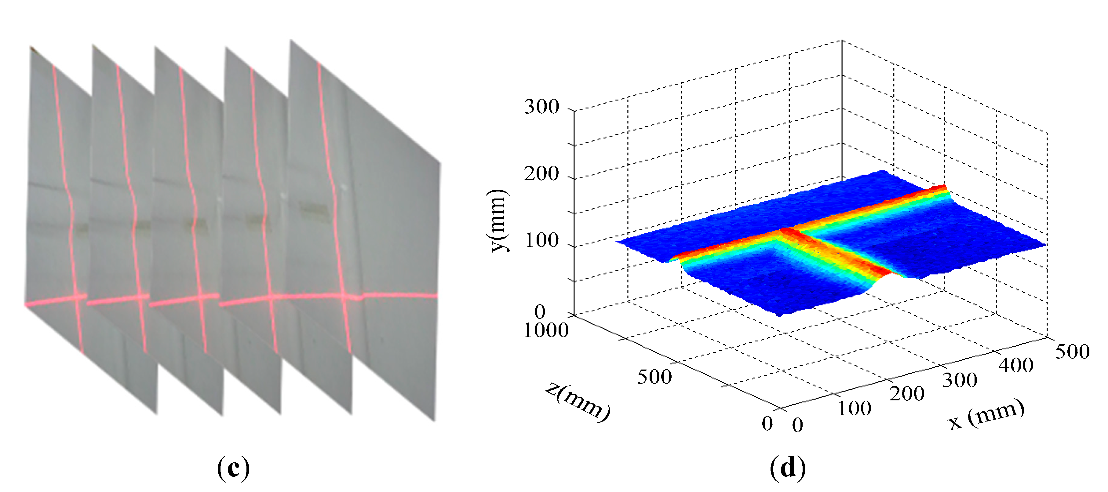
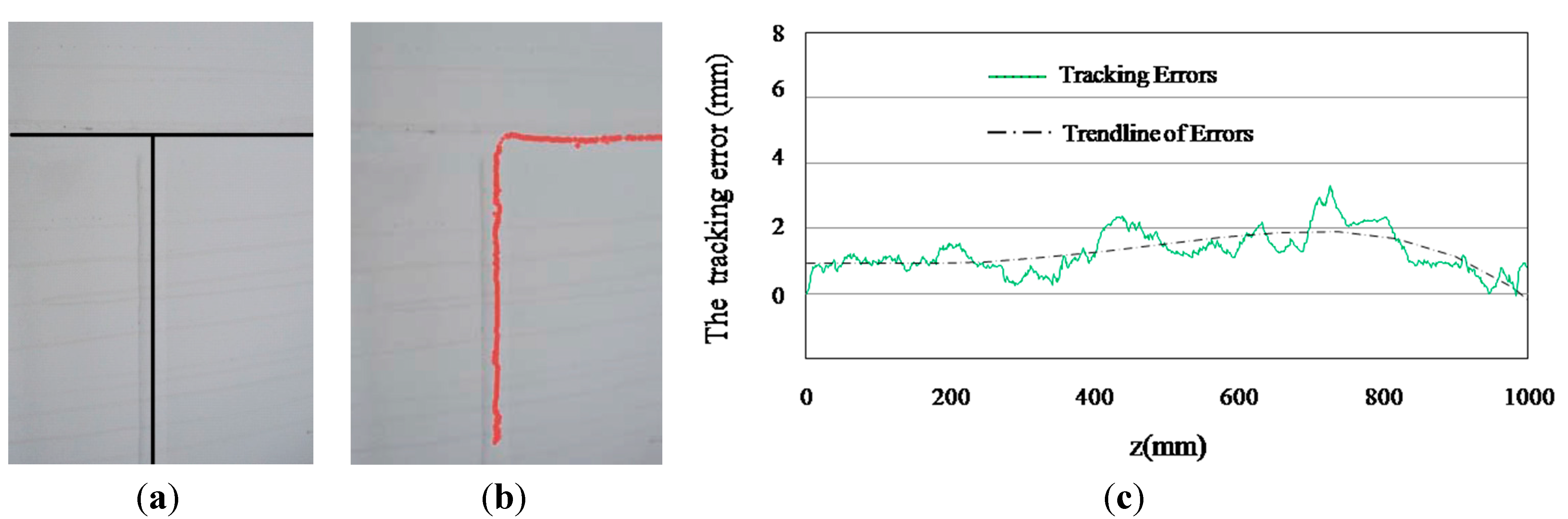
4.3. Weld Line Detection and Tracking of Wall Climbing Robot


5. Conclusions
Acknowledgments
Author Contributions
Conflicts of Interest
References
- Silberman, N.; Rob, F. Indoor scene segmentation using a structured light sensor. In Proceedings of the IEEE International Conference on Computer Vision Workshops, Barcelona, Spain, 6–13 November 2011; pp. 601–608.
- Park, J.B.; Lee, S.H.; Lee, J. Precise 3D lug pose detection sensor for automatic robot welding using a structured-light vision system. Sensors 2009, 9, 7550–7565. [Google Scholar] [CrossRef] [PubMed]
- Huang, W.; Radovan, K. A laser-based vision system for weld quality inspection. Sensors 2011, 11, 506–521. [Google Scholar] [CrossRef] [PubMed]
- Zhao, X.; Liu, H.; Yu, Y.; Xu, X.; Hu, W.; Li, M.; Ou, J. Bridge Displacement Monitoring Method Based on Laser Projection Sensing Technology. Sensors 2015, 15, 8444–8463. [Google Scholar] [CrossRef] [PubMed]
- Usamentiaga, R.; Molleda, J.; Garcia, D.F. Structured-Light Sensor Using Two Laser Stripes for 3D Reconstruction without Vibrations. Sensors 2014, 11, 20041–20063. [Google Scholar] [CrossRef] [PubMed]
- Barone, S.; Alessandro, P.; Armando, V.R. 3D Reconstruction and Restoration Monitoring of Sculptural Artworks by a Multi-Sensor Framework. Sensors 2012, 12, 16785–16801. [Google Scholar] [CrossRef] [PubMed]
- Zhan, D.; Yu, L.; Xiao, J.; Chen, T. Multi-Camera and Structured-Light Vision System (MSVS) for Dynamic High-Accuracy 3D Measurements of Railway Tunnels. Sensors 2015, 15, 8664–8684. [Google Scholar] [CrossRef] [PubMed]
- Bieri, L.S.; Jacques, J. Three-dimensional vision using structured light applied to quality control in production line. Proc. SPIE 2004, 5457. [Google Scholar] [CrossRef]
- Usamentiaga, R.; Molleda, J.; García, D.F.; Bulnes, F.G. Machine vision system for flatness control feedback. In Proceedings of the IEEE International Conference on Machine Vision, Dubai, The United Arab Emirates, 28–30 December 2009; pp. 105–110.
- Appia, V.; Pedro, G. Comparison of fixed-pattern and multiple-pattern structured light imaging systems. Proc. SPIE 2014, 8909. [Google Scholar] [CrossRef]
- Gupta, M.; Qi, Y.; Nayar, S.K. Structured light in sunlight. In Proceedings of the IEEE International Conference on Computer Vision, Sydney, Australia, 1–8 December 2013; pp. 545–552.
- O’TOOLE, M.; John, M.; Kutulakos, K.N. 3D shape and indirect appearance by structured light transport. In Proceedings of the 2014 IEEE Conference on Computer Vision and Pattern Recognition, Columbus, OH, USA, 23–28 June 2014; pp. 3246–3253.
- Liu, D.; Cheng, X.; Yang, Y.-H. Frequency-Based 3D Reconstruction of Transparent and Specular Objects. In Proceedings of the 2014 IEEE Conference on Computer Vision and Pattern Recognition, Columbus, OH, USA, 23–28 June 2014; pp. 660–667.
- Molleda, J.; Usamentiaga, R.; García, D.F.; Bulnes, F.G. Real-time flatness inspection of rolled products based on optical laser triangulation and three-dimensional surface reconstruction. J. Electron. Imaging 2010, 19, 031206. [Google Scholar] [CrossRef]
- Usamentiaga, R.; Molleda, J.; Garcia, D.F.; Bulnes, F.G. Removing vibrations in 3D reconstruction using multiple laser stripes. Opt. Lasers Eng. 2014, 53, 51–59. [Google Scholar] [CrossRef]
- Fisher, R.B.; Naidu, D.K. A comparison of algorithms for subpixel peak detection. In Image Technology; Springer: Berlin/Heidelberg, Germany, 1996; pp. 385–404. [Google Scholar]
- Haug, K.; Pritschow, G. Robust laser-stripe sensor for automated weld-seam-tracking in the shipbuilding industry. In Proceedings of the IEEE Annual Conference of the Industrial Electronics Society, Aachen, Germany, 31 August–4 September 1998; Volume 2, pp. 1236–1241.
- Strobl, K.H.; Sepp, W.; Wahl, E.; Bodenmuller, T.; Suppa, M.; Seara, J.F.; Hirzinger, G. The DLR multisensory hand-guided device: The laser stripe profiler. In Proceedings of the 2004 IEEE International Conference on Robotics and Automation, New Orleans, LA, USA, 26 April–1 May 2004; Volume 2, pp. 1927–1932.
- Li, Y.; Li, Y.F.; Wang, Q.L.; Xu, D.; Tan, M. Measurement and defect detection of the weld bead based on online vision inspection. IEEE Trans. Instrum. Meas. 2010, 59, 1841–1849. [Google Scholar]
- Molleda, J.; Usamentiaga, R.; Garcia, D.F.; Bulnes, F.G.; Ema, L. Shape measurement of steel strips using a laser-based three-dimensional reconstruction technique. IEEE Trans. Ind. Appl. 2011, 47, 1536–1544. [Google Scholar] [CrossRef]
- Usamentiaga, R.; Molleda, J.; García, D.F. Fast and robust laser stripe extraction for 3D reconstruction in industrial environments. Mach. Vis. Appl. 2012, 23, 179–196. [Google Scholar] [CrossRef]
- Ofner, R.; O’Leary, P.; Leitner, M. A collection of algorithms for the determination of construction points in the measurement of 3D geometries via light-sectioning. In Workshop on European Scientific and Industrial Collaboration: Advanced Technologies in Manufacturing; University of Wales College: Newport, UK, 1999; pp. 505–512. [Google Scholar]
- Forest, J.; Salvi, J.; Cabruja, E.; Pous, C. Laser stripe peak detector for 3D scanners. A FIR filter approach. In Proceedings of the IEEE International Conference on Pattern Recognition, Cambridge, UK, 23–26 August 2004; Volume 3, pp. 646–649.
- Schnee, J.; Futterlieb, J. Laser line segmentation with dynamic line models. In Computer Analysis of Images and Patterns; Springer: Berlin/Heidelberg, Germany, 2011; pp. 126–134. [Google Scholar]
- Steger, C. An unbiased detector of curvilinear structures. IEEE Trans. Pattern Anal. Mach. Intell. 1998, 20, 113–125. [Google Scholar] [CrossRef]
- Xu, D.; Wang, L.; Tu, Z.; Tan, M. Hybrid visual servoing control for robotic arc welding based on structured light vision. Acta. Autom. Sin. 2005, 31, 596. [Google Scholar]
- Zhang, L.; Ye, Q.; Yang, W.; Jiao, J. Weld line detection and tracking via spatial-temporal cascaded hidden Markov models and cross structured light. IEEE Trans. Instrum. Meas. 2014, 63, 742–753. [Google Scholar] [CrossRef]
- Sturm, P.; Ramalingam, S.; Tardif, J.P.; Gasparini, S.; Barreto, J. Camera models and fundamental concepts used in geometric computer vision. Found. Trends Comp. Graph. Vis. 2011, 6, 1–183. [Google Scholar] [CrossRef]
- Tsai, R.Y. A versatile camera calibration technique for high-accuracy 3D machine vision metrology using off-the-shelf TV cameras and lenses. IEEE J. Robot. Autom. 1987, 3, 323–344. [Google Scholar] [CrossRef]
- Medioni, G.; Kang, S.B. Emerging Topics in Computer Vision; Prentice Hall PTR: New York, NY, USA, 2004. [Google Scholar]
- Zhang, Z. A flexible new technique for camera calibration. IEEE Trans. Pattern Anal. Mach. Intell. 2000, 22, 1330–1334. [Google Scholar] [CrossRef]
- Moré, J.J. The Levenberg-Marquardt algorithm: Implementation and theory. In Numerical Analysis; Springer: Berlin/Heidelberg, Germany, 1978; pp. 105–116. [Google Scholar]
- Wiggins, R.A. Minimum entropy deconvolution. Geoexploration 1978, 16, 21–35. [Google Scholar] [CrossRef]
- McDonald, G.L.; Zhao, Q.; Zuo, M.J. Maximum correlated Kurtosis deconvolution and application on gear tooth chip fault detection. Mech. Syst. Signal Process. 2012, 33, 237–255. [Google Scholar] [CrossRef]
- Collins, R.T.; Liu, Y.; Leordeanu, M. Online selection of discriminative tracking features. IEEE Trans. Pattern Anal. Mach. Intell. 2005, 27, 1631–1643. [Google Scholar] [CrossRef] [PubMed]
- Ohta, Y.I.; Kanade, T.; Sakai, T. Color information for region segmentation. Comput. Graph.Image Process. 1980, 13, 222–241. [Google Scholar] [CrossRef]
- Bronstein, M.M.; Bronstein, A.M.; Zibulevsky, M.; Zeevi, Y.Y. Blind deconvolution of images using optimal sparse representations. IEEE Trans. Image Process. 2005, 14, 726–736. [Google Scholar] [CrossRef] [PubMed]
- González, G.; Badra, R.E.; Medina, R.; Regidor, J. Period estimation using minimum entropy deconvolution (MED). Signal Process. 1995, 41, 91–100. [Google Scholar] [CrossRef]
- Sawalhi, N.; Randall, R.B.; Endo, H. The enhancement of fault detection and diagnosis in rolling element bearings using minimum entropy deconvolution combined with spectral kurtosis. Mech. Syst. Signal Process. 2007, 21, 2616–2633. [Google Scholar] [CrossRef]
- Nandi, A.K.; Mämpel, D.; Roscher, B. Blind deconvolution of ultrasonic signals in nondestructive testing applications. IEEE Trans. Signal Process. 1997, 45, 1382–1390. [Google Scholar] [CrossRef]
- Boumahdi, M.; Lacoume, J.L. Blind identification using the Kurtosis: Results of field data processing. In Proceedings of the IEEE International Conference on Acoustics, Speech, and Signal Processing, Detroit, MI, USA, 9–12 May 1995; Volume 3, pp. 1980–1983.
- Donoho, D. On minimum entropy deconvolution. In Applied Time Series Analysis II; Elsevier: Amsterdam, The Netherlands, 1981; pp. 565–608. [Google Scholar]
- Zhou, F.; Peng, B.; Cui, Y.; Wang, Y.; Tan, H. A novel laser vision sensor for omnidirectional 3D measurement. Opt. Laser Technol. 2013, 45, 1–12. [Google Scholar] [CrossRef]
© 2015 by the authors; licensee MDPI, Basel, Switzerland. This article is an open access article distributed under the terms and conditions of the Creative Commons Attribution license (http://creativecommons.org/licenses/by/4.0/).
Share and Cite
Zhang, L.; Sun, J.; Yin, G.; Zhao, J.; Han, Q. A Cross Structured Light Sensor and Stripe Segmentation Method for Visual Tracking of a Wall Climbing Robot. Sensors 2015, 15, 13725-13751. https://doi.org/10.3390/s150613725
Zhang L, Sun J, Yin G, Zhao J, Han Q. A Cross Structured Light Sensor and Stripe Segmentation Method for Visual Tracking of a Wall Climbing Robot. Sensors. 2015; 15(6):13725-13751. https://doi.org/10.3390/s150613725
Chicago/Turabian StyleZhang, Liguo, Jianguo Sun, Guisheng Yin, Jing Zhao, and Qilong Han. 2015. "A Cross Structured Light Sensor and Stripe Segmentation Method for Visual Tracking of a Wall Climbing Robot" Sensors 15, no. 6: 13725-13751. https://doi.org/10.3390/s150613725
APA StyleZhang, L., Sun, J., Yin, G., Zhao, J., & Han, Q. (2015). A Cross Structured Light Sensor and Stripe Segmentation Method for Visual Tracking of a Wall Climbing Robot. Sensors, 15(6), 13725-13751. https://doi.org/10.3390/s150613725