
Reducing Systematic Centroid Errors Induced by Fiber Optic Faceplates in Intensified High-Accuracy Star Trackers

Abstract
:1. Introduction
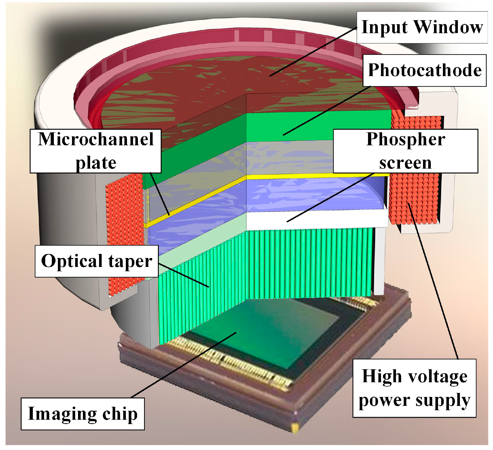
2. Optoelectronic Detecting System of Intensified High-Accuracy Star Trackers
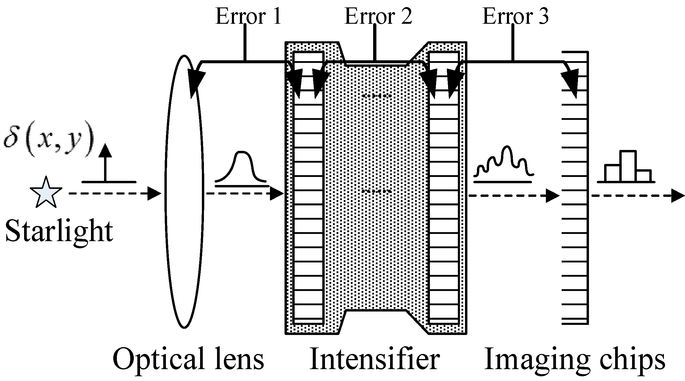
2.1. Imaging Principle

2.2. FOFP-Induced Centroid Error
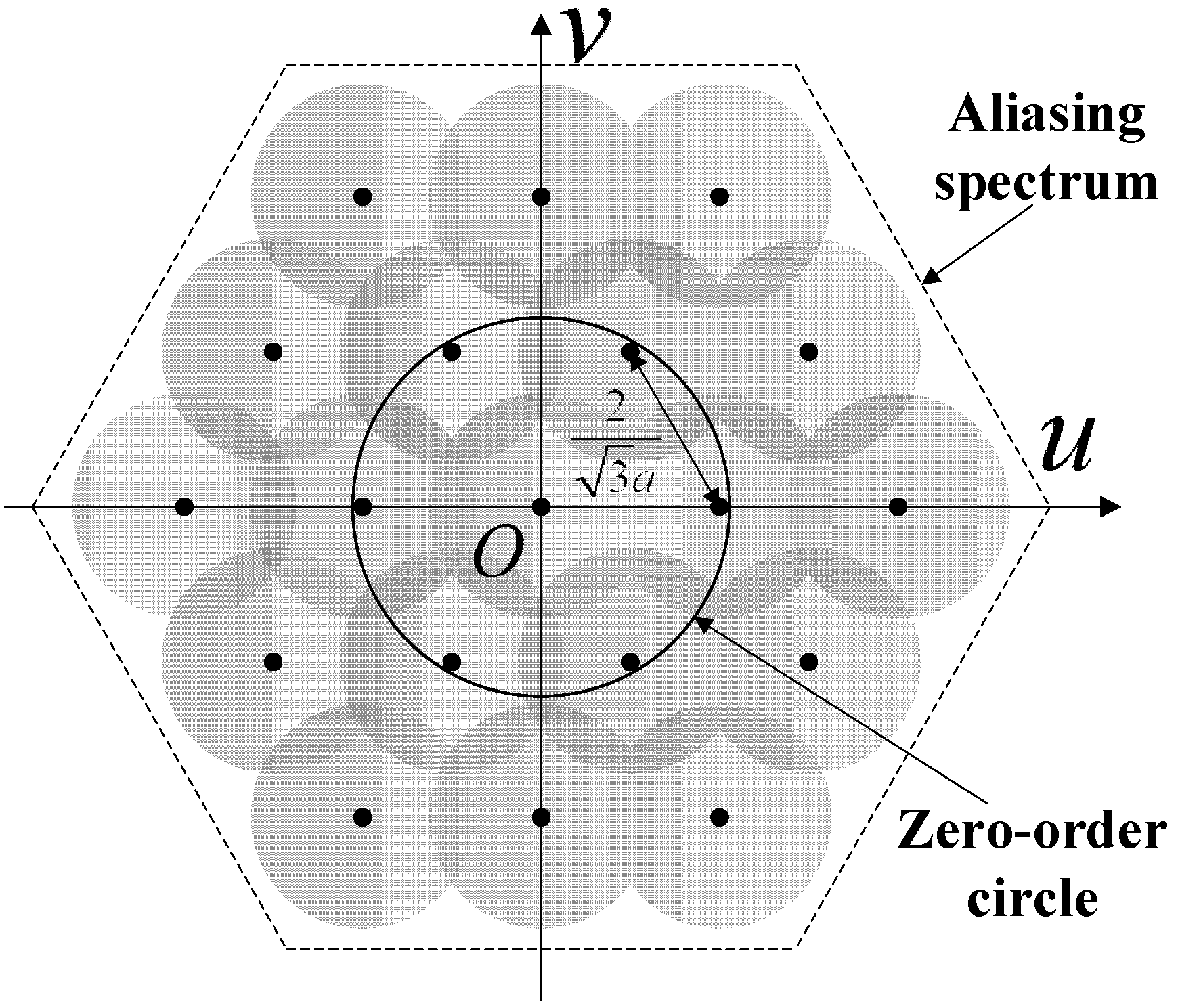
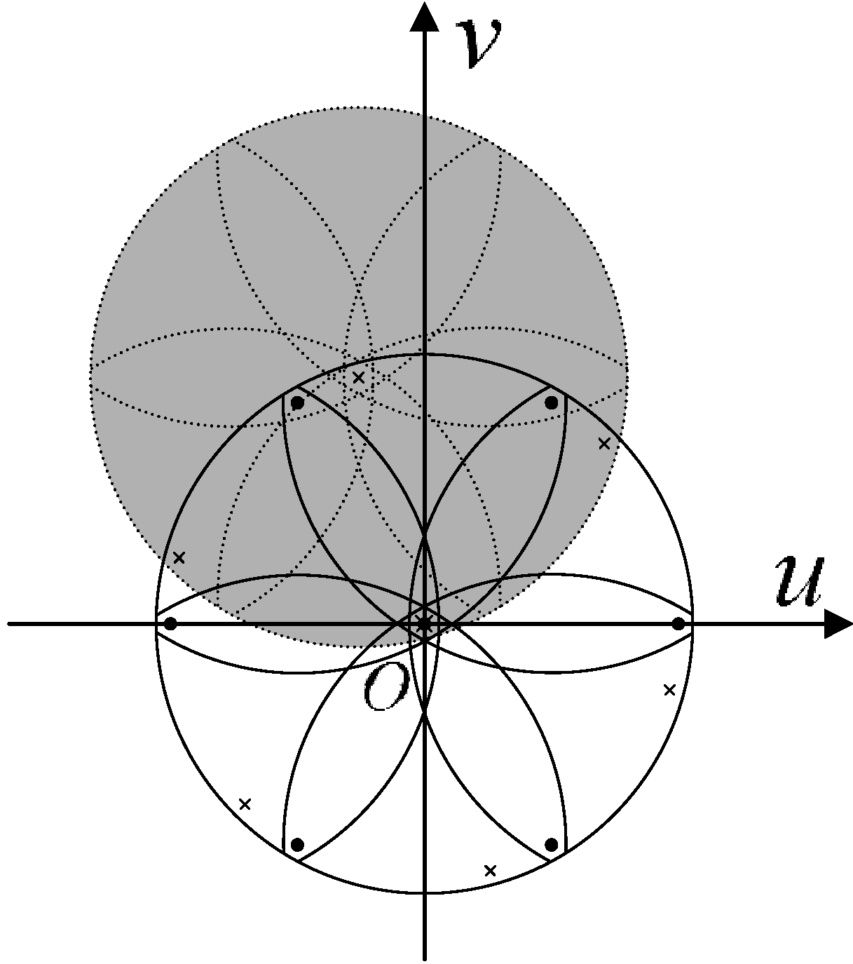
3. Frequency Domain Analysis of Centroid Localization
3.1. Centroid Localization Expression in the Frequency Domain
3.2. Systematic Centroid Error Expression
4. Image Transmission Model of FOFP


5. Reducing FOFP-Induced Systematic Centroid Errors
5.1. Systematic Error Reduction between the Optical Lens and the Input FOFP of an Intensifier
5.1.1. Optical Lens Analysis
5.1.2. Systematic Centroid Error of an FOFP

5.1.3. Error Reduction
5.2. Systematic Error Reduction among Multiple FOFPs

5.3. Systematic Error Reduction between the Output FOFP of the Intensifier and the Imaging Chip
6. Simulations and Experiments
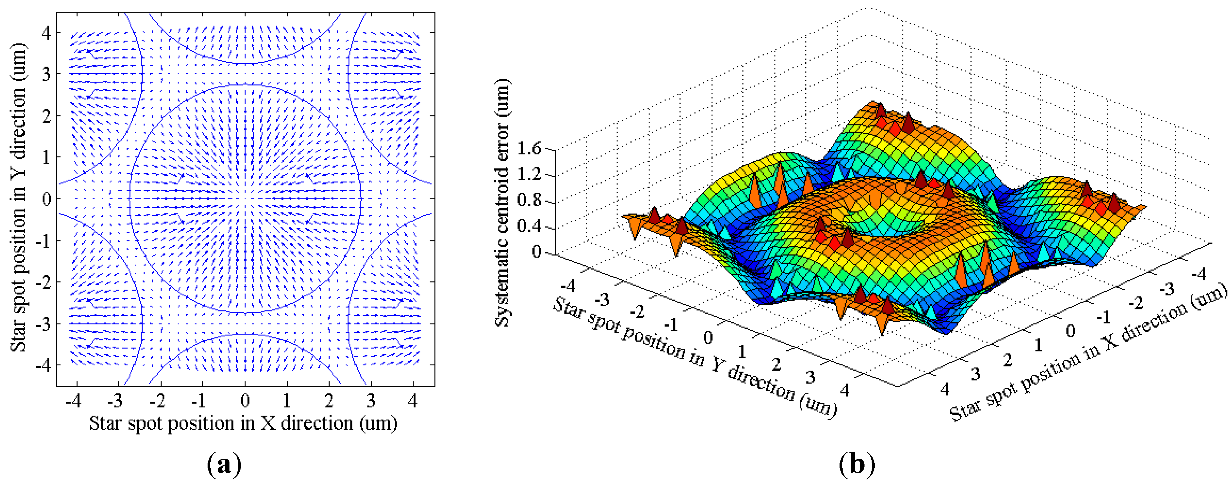
6.1. Simulation of the Systematic Centroid Error of an FOFP

| Parameters | Values |
|---|---|
| Fiber core diameter | 5.5 μm |
| Fiber interval | 6 μm |
| Star spot diameter | 12 μm |
| Simulation area | 20 μm × 20 μm |
| Test star spot density | 0.2 μm |

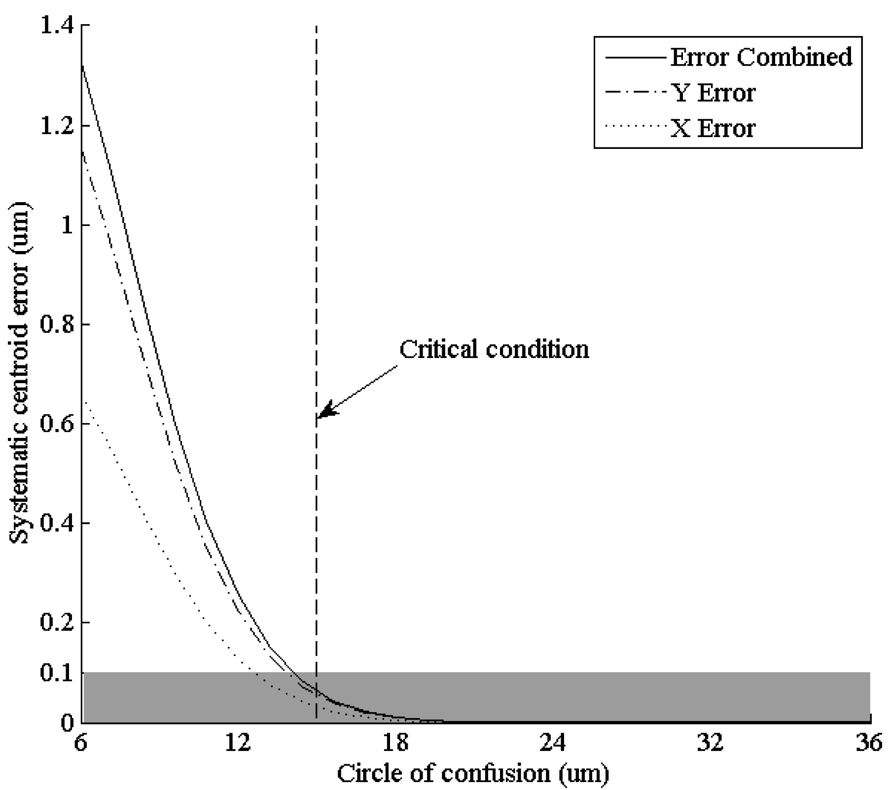
6.2. Simulation of the Match between the Optical Lens and the Input FOFP of the Intensifier


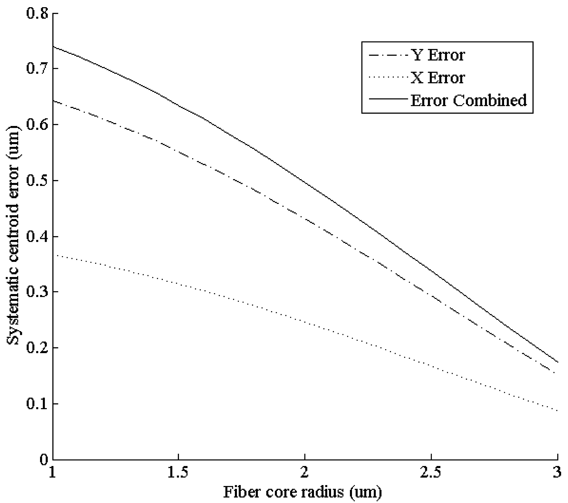
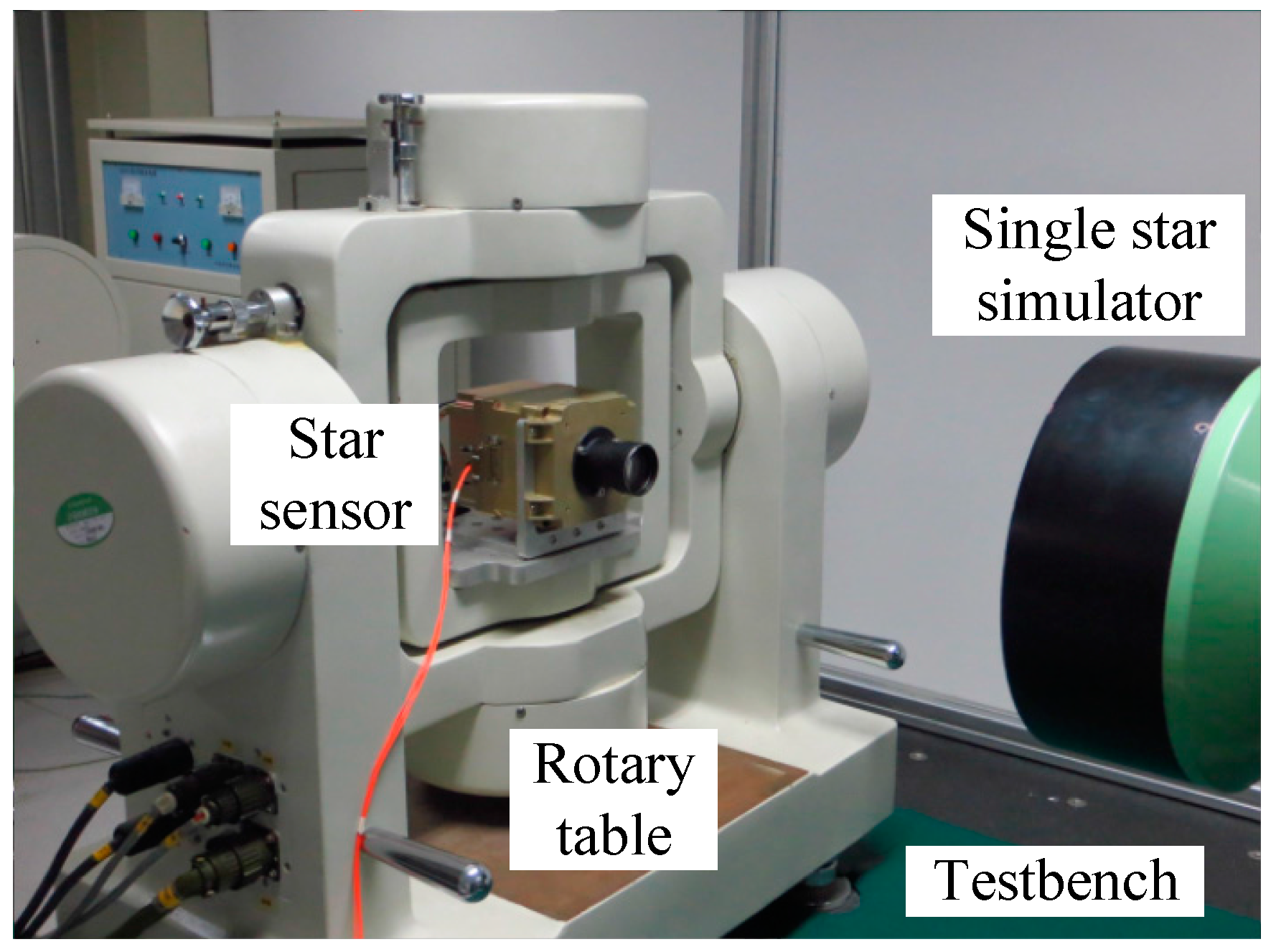
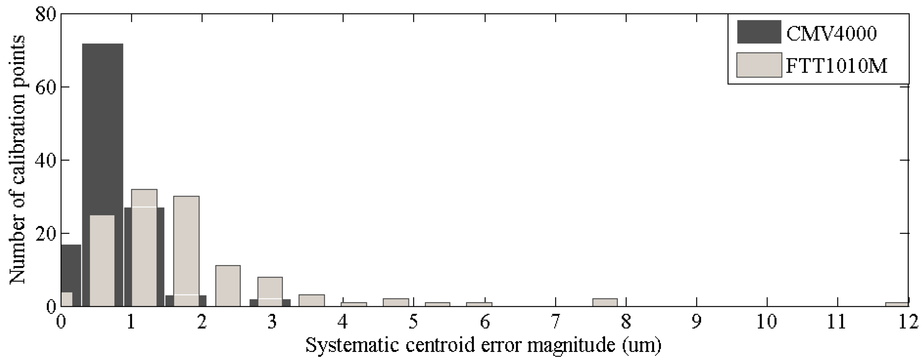
6.3. Experimental Investigation on the Match between the Output FOFP of the Intensifier and the Imaging Chip
| Chip Name | FTT1010M | CMV4000 |
|---|---|---|
| Manufacturer | Dalsa Inc. | CMOSIS Co. |
| Chip Type | Frame Transfer CCD | CMOS |
| Pixel Size | 12 μm × 12 μm | 5.5 μm × 5.5 μm |
| Image Size | 1024 × 1024 pixels (12.288 mm × 12.288 mm) | 2048 × 2048 pixels (11.264 mm × 11.264 mm) |
7. Conclusions
Acknowledgments
Author Contributions
Conflicts of Interest
References
- Eisenman, A.R.; Liebe, C.C. The advancing state-of-the-art in second generation star trackers. In Proceedings of the 1998 IEEE Aerospace Conference, Snowmass at Aspen, CO, USA, 21–28 March 1998; pp. 111–118.
- Steyn, W.; Jacobs, M.; Oosthuizen, P. A high performance star sensor system for full attitude determination on a microsatellite. In Proceedings of the Workshop on Control of Small Spacecraft at the 1997 Annual AAS Guidance and Control Conference, Breckenridge, CO, USA, 5 February 1997.
- Liebe, C.C.; Alkalai, L.; Domingo, G.; Hancock, B.; Hunter, D.; Mellstrom, J.; Ruiz, I.; Sepulveda, C.; Pain, B. Micro APS based star tracker. In Proceedings of the 2002 IEEE Aerospace Conference Proceedings, Pasadena, CA, USA, 9–16 March, 2002; Volume 2285.
- Liebe, C.C.; Gromov, K.; Meller, D.M. Toward a stellar gyroscope for spacecraft attitude determination. J. Guid. Control Dyn. 2004, 27, 91–99. [Google Scholar] [CrossRef]
- Katake, A.; Bruccoleri, C. StarCam SG100: A high-update rate, high-sensitivity stellar gyroscope for spacecraft. IS&T/SPIE Electron. Imaging 2010. [Google Scholar] [CrossRef]
- Zhang, H.; Li, J. The effects of APS star tracker detection sensitivity. In Proceedings of the International Conference of Optical Instrument and Technology, Beijing, China, 16–19 November 2008; pp. 71601F–71608F.
- Shen, J.; Zhang, G.; Wei, X. Simulation analysis of dynamic working performance for star trackers. JOSA A 2010, 27, 2638–2647. [Google Scholar] [CrossRef] [PubMed]
- Wei, X.; Tan, W.; Li, J.; Zhang, G. Exposure Time Optimization for Highly Dynamic Star Trackers. Sensors 2014, 14, 4914–4931. [Google Scholar] [CrossRef] [PubMed]
- Player, M. Spread functions and modulation transfer functions of fiber-optic bundles. J. Mod. Opt. 1988, 35, 1363–1372. [Google Scholar] [CrossRef]
- Barnard, K.J.; Boreman, G.D. Modulation transfer function of hexagonal staring focal plane arrays. Opt. Eng. 1991, 30, 1915–1919. [Google Scholar] [CrossRef]
- Zhang, W.; Wang, Y.; Tian, W.; Ma, W.; Zhang, H.; Sun, A. Novel methods for measuring modulation transfer function for fiber optic taper. In Proceedings of the ICO20: Optical Design and Fabrication, Changchun, China, 31 January, 2006; pp. 603413–603417.
- Li, H.; Chen, B.; Feng, K.; Ma, H. Modulation transfer function measurement method for fiber optic imaging bundles. Opt. Laser Technol. 2008, 40, 415–419. [Google Scholar] [CrossRef]
- Yang, X.; Tang, Y.; Liu, K.; Liu, H.; Gao, H.; Li, Q. Modulation transfer function of partial gating detector by liquid crystal auto-controlling light intensity. In Proceedings of the Photonics and Optoelectronics Meetings, Wuhan, China, 11 December 2008; pp. 72790Z–72798Z.
- Liebe, C.C. Accuracy performance of star trackers-a tutorial. IEEE Trans. Aerosp. Electron. Syst. 2002, 38, 587–599. [Google Scholar] [CrossRef]
- Yang, J.; Liang, B.; Zhang, T.; Song, J. A novel systematic error compensation algorithm based on least squares support vector regression for star sensor image centroid estimation. Sensors 2011, 11, 7341–7363. [Google Scholar] [CrossRef] [PubMed]
- Katake, A.B. Modeling, Image Processing and Attitude Estimation of High Speed Star Sensors. Ph.D. Thesis, Texas A&M University, College Station, TX, USA, 2006. [Google Scholar]
- Alexander, B.F.; Ng, K.C. Elimination of systematic error in subpixel accuracy centroid estimation. Opt. Eng. 1991, 30, 1320–1331. [Google Scholar] [CrossRef]
© 2015 by the authors; licensee MDPI, Basel, Switzerland. This article is an open access article distributed under the terms and conditions of the Creative Commons Attribution license (http://creativecommons.org/licenses/by/4.0/).
Share and Cite
Xiong, K.; Jiang, J. Reducing Systematic Centroid Errors Induced by Fiber Optic Faceplates in Intensified High-Accuracy Star Trackers. Sensors 2015, 15, 12389-12409. https://doi.org/10.3390/s150612389
Xiong K, Jiang J. Reducing Systematic Centroid Errors Induced by Fiber Optic Faceplates in Intensified High-Accuracy Star Trackers. Sensors. 2015; 15(6):12389-12409. https://doi.org/10.3390/s150612389
Chicago/Turabian StyleXiong, Kun, and Jie Jiang. 2015. "Reducing Systematic Centroid Errors Induced by Fiber Optic Faceplates in Intensified High-Accuracy Star Trackers" Sensors 15, no. 6: 12389-12409. https://doi.org/10.3390/s150612389
APA StyleXiong, K., & Jiang, J. (2015). Reducing Systematic Centroid Errors Induced by Fiber Optic Faceplates in Intensified High-Accuracy Star Trackers. Sensors, 15(6), 12389-12409. https://doi.org/10.3390/s150612389