
True Colour Classification of Natural Waters with Medium-Spectral Resolution Satellites: SeaWiFS, MODIS, MERIS and OLCI


Abstract
:1. Introduction
2. Material and Methods
2.1. Satellite Colourimetry
2.2. Data
2.2.1. Synthetic Spectra

| Instrument | SeaWiFS | MODIS Aqua | MERIS | Sentinel 3 OLCI |
|---|---|---|---|---|
| Operational | September 1997–December 2010 | May 2002–present | May 2002–April 2012 | End 2015– |
| Spatial Res. | 1100 m | 1000 m | 300 m | 300 m |
| Band nr. | Wavelength/Bandwidth | |||
| 1 | 412/20 | 412.5/10 | 400/15 | |
| 2 | 443/20 | 442.5/10 | 412.5/10 | |
| 3 | 490/20 | 490/10 | 442.5/10 | |
| 4 | 510/20 | 510/10 | 490/10 | |
| 5 | 555/20 | 560/10 | 510/10 | |
| 6 | 670/20 | 620/10 | 560/10 | |
| 7 | 765/40 | 665/10 | 620/10 | |
| 8 | 412.5/15 | 681.25/7.5 | 665/10 | |
| 9 | 443/10 | 708.75/10 | 673.5/7.5 | |
| 10 | 488/10 | 753.75/7.5 | 681.25/7.5 | |
| 11 | 531/10 | 708.75/10 | ||
| 12 | 551/10 | 753.75/7.5 | ||
| 13 | 667/10 | |||
| 14 | 678/10 | |||
| 15 | 748/10 | |||
2.2.2. TriOS Spectra
2.2.3. Satellite Data
3. Results
3.1. Simulation Spectra
| ME-Band | 1 | 2 | 3 | 4 | 5 | 6 | 7 | 8 | 9 | ||
|---|---|---|---|---|---|---|---|---|---|---|---|
| λ (nm) | 400 | 412.5 | 442.5 | 490 | 510 | 560 | 620 | 665 | 681.25 | 708 | 710 |
| xME | 0.154 | 2.813 | 10.867 | 3.883 | 3.750 | 34.687 | 41.853 | 7.619 | 0.844 | 0.189 | 0.006 |
| yME | 0.004 | 0.104 | 1.687 | 5.703 | 23.263 | 48.791 | 23.949 | 2.944 | 0.307 | 0.068 | 0.002 |
| zME | 0.731 | 13.638 | 58.288 | 29.011 | 4.022 | 0.618 | 0.026 | 0.000 | 0.000 | 0.000 | 0.000 |

| OL-Band | 1 | 2 | 3 | 4 | 5 | 6 | 7 | 8 | 9 | 10 | 11 | |
| λ (nm) | 400 | 413 | 443 | 490 | 510 | 560 | 620 | 665 | 673.5 | 681.25 | 708.75 | 710 |
| xOL | 0.154 | 2.957 | 10.861 | 3.744 | 3.750 | 34.687 | 41.853 | 7.323 | 0.591 | 0.549 | 0.189 | 0.006 |
| yOL | 0.004 | 0.112 | 1.711 | 5.672 | 23.263 | 48.791 | 23.949 | 2.836 | 0.216 | 0.199 | 0.068 | 0.002 |
| zOL | 0.731 | 14.354 | 58.356 | 28.227 | 4.022 | 0.618 | 0.026 | 0.000 | 0.000 | 0.000 | 0.000 | 0.000 |
| MO-Band | 8 | 9 | 10 | 11 | 12 | 13 | 14 | |||||
| λ (nm) | 400 | 412.5 | 443 | 490 | 531 | 551 | 667 | 678 | 710 | |||
| xMO | 0.154 | 2.957 | 10.861 | 4.031 | 3.989 | 49.037 | 34.586 | 0.829 | 0.222 | |||
| yMO | 0.004 | 0.112 | 1.711 | 11.106 | 22.579 | 51.477 | 19.452 | 0.301 | 0.080 | |||
| zMO | 0.731 | 14.354 | 58.356 | 29.993 | 2.618 | 0.262 | 0.022 | 0.000 | 0.000 | |||
| SW-Band | 1 | 2 | 3 | 4 | 5 | 6 | ||||||
| λ (nm) | 400 | 413 | 443 | 490 | 510 | 555 | 670 | 710 | ||||
| xSW | 0.154 | 2.957 | 10.861 | 3.744 | 3.455 | 52.304 | 32.825 | 0.364 | ||||
| ySW | 0.004 | 0.112 | 1.711 | 5.672 | 21.929 | 59.454 | 17.810 | 0.132 | ||||
| zSW | 0.731 | 14.354 | 58.356 | 28.227 | 3.967 | 0.682 | 0.018 | 0.000 |
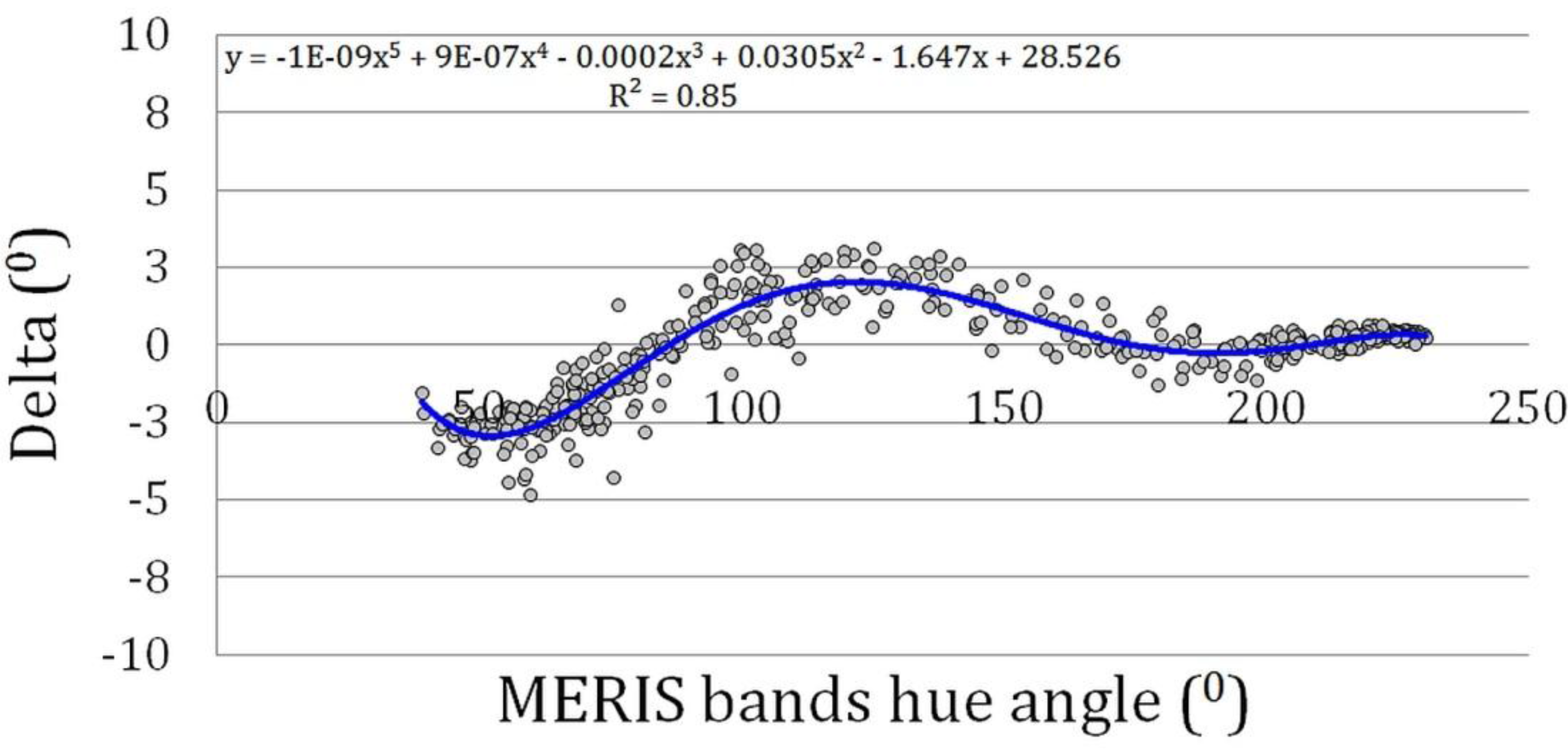
| Instrument | a5 | a4 | a3 | a2 | a1 | Constant |
|---|---|---|---|---|---|---|
| MERIS | −12.0506 | 88.9325 | −244.6960 | 305.2361 | −164.6960 | 28.5255 |
| OLCI | −12.5076 | 91.6345 | −249.8480 | 308.6561 | −165.4818 | 28.5608 |
| MODISA | −48.0880 | 362.6179 | −1011.7151 | 1262.0348 | −666.5981 | 113.9215 |
| SeaWiFS | −49.4377 | 363.2770 | −978.1648 | 1154.6030 | −552.2701 | 78.2940 |
3.2. Field Spectra
3.3. Satellite Inter-Comparison

4. Discussion and Conclusions
Supplementary Files
Supplementary File 1Acknowledgments
Author Contributions
Conflicts of Interest
References
- Remote Sensing of Ocean Colour in Coastal, Other Optically-Complex Waters. In Reports of the International Ocean Colour Coordinating Group; No. 3; Sathyendranath, S. (Ed.) IOCCG: Darmouth, NS, Canada, 2000.
- Remote Sensing of Inherent Optical Properties: Fundamentals, Tests of Algorithms, and Applications. In Reports of the International Ocean-Colour Coordinating Group; No. 5; Lee, Z.P. (Ed.) IOCCG: Dartmouth, NS, Canada, 2006.
- Lee, Z.P.; Carder, K.; Arnone, R.; He, M. Determination of Primary Spectral Bands for Remote Sensing of Aquatic Environments. Sensors 2007, 7, 3428–3441. [Google Scholar] [CrossRef]
- Odermat, D.; Gitelson, A.; Brando, V.E.; Schaepman, M. Review of constituent retrieval in optically deep and complex waters from satellite imagery. Remote Sens. Environ. 2012, 118, 116–126. [Google Scholar] [CrossRef]
- Van der Woerd, H.J.; Pasterkamp, R. HYDROPT: A fast and flexible method to retrieve chlorophyll-a from multispectral satellite observations of optically complex coastal waters. Remote Sens. Environ. 2008, 112, 1795–1807. [Google Scholar] [CrossRef]
- Commission Internationale de l’Éclairage Proceedings, 1931; Cambridge University Press: Cambridge, UK, 1932.
- Wernand, M.R.; van der Woerd, H.J. Spectral analyses of the Forel-Ule ocean colour comparator scale. J. Eur. Opt. Soc. Rap. Public 2010, 5, 1–7. [Google Scholar] [CrossRef]
- Citclops Project Website. Available online: http://www.citclops.eu/ (accessed on 10 August 2015).
- Novoa, S.; Wernand, M.; van der Woerd, H.J. The Forel-Ule scale converted to modern tools for participatory water quality monitoring. In Proceedings of the Extended Abstract Ocean Optics Conference XXII, Portland, OR, USA, 20 October 2014.
- Kirk, J.T.O. Light and Photosynthesis in Aquatic Ecosystems, 3rd ed.; Cambridge University Press: Cambridge, UK, 2011. [Google Scholar]
- Mobley, C.D. Light and Water: Radiative Transfer in Natural Waters; Academic Press: San Diego, CA, USA, 1994. [Google Scholar]
- Wernand, M.R.; Hommersom, A.; van der Woerd, H.J. MERIS-based ocean colour classification with the discrete Forel-Ule scale. Ocean Sci. 2013, 9, 477–487. [Google Scholar] [CrossRef]
- IOCCG Data. Available online: http://www.ioccg.org/groups/OCAG_data.html (accessed on 10 August 2015).
- Wyszecki, G.; Stiles, W.S. Colour Science: Concepts and Methods, Quantitative Data and Formulae; John Wiley & Sons: New York, NY, USA, 1982. [Google Scholar]
- Novoa, S.; Wernand, M.; van der Woerd, H.J. WACODI: A generic algorithm to derive the intrinsic color of natural waters from digital images. Limnol. Oceanogr. Meth. 2015, in press. [Google Scholar] [CrossRef]
- Mobley, C.D. Hydrolight 3.0 Users’ Guide; SRI International: Menlo Park, CA, USA, 1995. [Google Scholar]
- Salama, Mhd. S.; Mélin, F.; van der Velde, R. Ensemble uncertainty of inherent optical properties. Opt. Express 2011, 19, 16772–16783. [Google Scholar]
- Dogliotti, A.I.; Ruddick, K.G.; Nechad, B.; Doxaran, D.; Knaeps, E. A single algorithm to retrieve turbidity from remotely-sensed data in all coastal and estuarine waters. Remote Sens. Environ. 2015, 156, 157–168. [Google Scholar] [CrossRef]
- Nechad, B.; Ruddick, K.G.; Park, Y. Calibration and validation of a generic multisensor algorithm for mapping of total suspended matter in turbid waters. Remote Sens. Environ. 2010, 114, 854–866. [Google Scholar] [CrossRef]
- Mueller, J.L.; Fargion, G.S.; Mcclain, C.R.; Mueller, J.L.; Morel, A.; Frouin, R.; Davis, C.; Arnone, R.; Carder, K.; Steword, R.G.; et al. Volume III : Radiometric Measurements and Data Analysis Protocols. In Ocean Optics Protocols for Satellite Ocean Color Sensor Validation; Revision 4; NASA: Washington DC, USA, 2003. [Google Scholar]
- VISAT BEAM. Available online: http://www.brockmann-consult.de/cms/web/beam/ (accessed on 10 August 2015).
- Lee, Z.P.; Carder, K.L.; Hawes, S.K.; Steward, R.G.; Peacock, T.G.; Davis, C.O. Model for the interpretation of hyperspectral remote-sensing reflectance. Appl. Opt. 1994, 33, 5721–5732. [Google Scholar] [CrossRef] [PubMed]
- Tilstone, G.; Peters, S.W.M.; van der Woerd, H.; Eleveld, M.; Ruddick, K.; Schoenfeld, W.; Krasemann, H.; Martinez-Vicente, V.; Blondeau-Patissier, D.; Röttgers, R.; et al. Variability in specific-absorption properties and their use in a semi-analytical Ocean Colour algorithm for MERIS in North Sea and Western English Channel Coastal Waters. Remote Sens. Environ. 2012, 118, 320–338. [Google Scholar] [CrossRef]
- Morel, A.; Antoine, D. MERIS ATBD. 2.9. Pigment Index Retrieval in Case 1 Waters; ESA: Frascati, Italy, 2011. [Google Scholar]
- Novoa, S.; Wernand, M.R.; van der Woerd, H.J. The Forel-Ule scale revisited spectrally: Preparation protocols, transmission measurements and chromaticity. J. Eur. Opt. Soc. Rap. Public 2013. [Google Scholar] [CrossRef]
- Wernand, M.R.; van der Woerd, H.J.; Gieskes, W.W.C. Trends in Ocean Colour and Chlorophyll Concentration from 1889 to 2000, Worldwide. PLoS ONE 2013, 8. [Google Scholar] [CrossRef]
- Zibordi, G.; Holben, B.; Mélin, F.; D’Alimonte, D.; Berthon, J.F.; Slutsker, I.; Giles, D. AERONET-OC: An overview. Can. J. Remote Sens. 2010, 36, 488–497. [Google Scholar] [CrossRef]
- Salama, M.S.; Su, B. Bayesian Model for Matching the Radiometric Measurements of Aerospace and Field Ocean Color Sensors. Sensors 2010, 10, 7561–7575. [Google Scholar] [CrossRef] [PubMed]
© 2015 by the authors; licensee MDPI, Basel, Switzerland. This article is an open access article distributed under the terms and conditions of the Creative Commons Attribution license (http://creativecommons.org/licenses/by/4.0/).
Share and Cite
Woerd, H.J.v.d.; Wernand, M.R. True Colour Classification of Natural Waters with Medium-Spectral Resolution Satellites: SeaWiFS, MODIS, MERIS and OLCI. Sensors 2015, 15, 25663-25680. https://doi.org/10.3390/s151025663
Woerd HJvd, Wernand MR. True Colour Classification of Natural Waters with Medium-Spectral Resolution Satellites: SeaWiFS, MODIS, MERIS and OLCI. Sensors. 2015; 15(10):25663-25680. https://doi.org/10.3390/s151025663
Chicago/Turabian StyleWoerd, Hendrik J. van der, and Marcel R. Wernand. 2015. "True Colour Classification of Natural Waters with Medium-Spectral Resolution Satellites: SeaWiFS, MODIS, MERIS and OLCI" Sensors 15, no. 10: 25663-25680. https://doi.org/10.3390/s151025663
APA StyleWoerd, H. J. v. d., & Wernand, M. R. (2015). True Colour Classification of Natural Waters with Medium-Spectral Resolution Satellites: SeaWiFS, MODIS, MERIS and OLCI. Sensors, 15(10), 25663-25680. https://doi.org/10.3390/s151025663