Comparability of Red/Near-Infrared Reflectance and NDVI Based on the Spectral Response Function between MODIS and 30 Other Satellite Sensors Using Rice Canopy Spectra


Abstract
: Long-term monitoring of regional and global environment changes often depends on the combined use of multi-source sensor data. The most widely used vegetation index is the normalized difference vegetation index (NDVI), which is a function of the red and near-infrared (NIR) spectral bands. The reflectance and NDVI data sets derived from different satellite sensor systems will not be directly comparable due to different spectral response functions (SRF), which has been recognized as one of the most important sources of uncertainty in the multi-sensor data analysis. This study quantified the influence of SRFs on the red and NIR reflectances and NDVI derived from 31 Earth observation satellite sensors. For this purpose, spectroradiometric measurements were performed for paddy rice grown under varied nitrogen levels and at different growth stages. The rice canopy reflectances were convoluted with the spectral response functions of various satellite instruments to simulate sensor-specific reflectances in the red and NIR channels. NDVI values were then calculated using the simulated red and NIR reflectances. The results showed that as compared to the Terra MODIS, the mean relative percentage difference (RPD) ranged from −12.67% to 36.30% for the red reflectance, −8.52% to −0.23% for the NIR reflectance, and −9.32% to 3.10% for the NDVI. The mean absolute percentage difference (APD) compared to the Terra MODIS ranged from 1.28% to 36.30% for the red reflectance, 0.84% to 8.71% for the NIR reflectance, and 0.59% to 9.32% for the NDVI. The lowest APD between MODIS and the other 30 satellite sensors was observed for Landsat5 TM for the red reflectance, CBERS02B CCD for the NIR reflectance and Landsat4 TM for the NDVI. In addition, the largest APD between MODIS and the other 30 satellite sensors was observed for IKONOS for the red reflectance, AVHRR1 onboard NOAA8 for the NIR reflectance and IKONOS for the NDVI. The results also indicated that AVHRRs onboard NOAA7-17 showed higher differences than did the other sensors with respect to MODIS. A series of optimum models were presented for remote sensing data assimilation between MODIS and other sensors.1. Introduction
In the past several decades, satellite remote sensing has played a vital role in providing up-to-date and detailed information for monitoring atmospheric and terrestrial environments at the regional, continental, and global scales. Such information is typically generated based on remotely sensed images processed into spectral vegetation indices [1,2]. Among the various spectral vegetation indices derived from remotely sensed imagery, one of the most widely used vegetation indices is the normalized difference vegetation index (NDVI), which is defined as the difference between the red and near-infrared (NIR) reflectance divided by their sum [3,4]. Previous studies showed that NDVI is strongly related to the fraction of absorbed photosynthetically active radiation (FPAR) [5,6], leaf area index (LAI) [7], and net primary production (NPP) [8–11]. NDVI has also been used in a range of applications including the study of vegetation–climate interactions [12–14], detection of long-term vegetation changes [15,16], assessment of vegetation functional characteristics [17–19] and modeling of the global carbon balance [10,20]. Furthermore, NDVI time series data has been successfully used in a variety of applications, including global change investigations, phenological studies, crop growth monitoring and yield prediction, drought and desertification monitoring, wildfire assessment, and climatic and biogeochemical modeling.
Since the launch of the National Oceanic and Atmospheric Administration (NOAA) satellites in 1970s, a large amount of invaluable and irreplaceable data sets have been available for global vegetation monitoring [21]. The Advanced Very High Resolution Radiometer (AVHRR) sensors onboard the NOAA satellites have provided one of the most extensive time series of remotely sensed data and continue to produce daily information regarding surface and atmospheric conditions [22]. Recently, the Moderate Resolution Imaging Spectroradiometer (MODIS) sensors onboard Terra and Aqua, designed to succeed the AVHRR instrument, has been of great importance for monitoring ecosystem variability and responses to seasonal and inter-annual environmental changes due to the improvement of both the temporal and spectral resolution relative to AVHRR. Sensors of this type, such as NOAA-AVHRR and EOS-MODIS, are appropriate for obtaining time-series data and provide more opportunities for acquiring cloud-free images by the use of composite images collected within a short period, although they are unable to avoid the influence of frequent heavy cloud cover. Many studies have demonstrated the application of these sensors to obtain large-area land-cover information [2,23–29]. Sensors of the other type, such as the Thematic Mapper/Enhanced Thematic Mapper (TM/ETM+) onboard Landsat, the High Resolution Visible/High Resolution Geometric (HRV/HRG) onboard Satellite Pour l'Observation de la Terre (SPOT), the Advanced Spaceborne Thermal Emission and Reflection Radiometer (ASTER) onboard Terra and the charge-coupled device (CCD) onboard the China Brazil Earth Resources Satellite (CBERS), have a relatively high spatial resolution, but small coverage and long revisit period. These instruments are appropriate for obtaining only detailed local information due to incomplete spatial coverage, infrequent temporal coverage with inevitable cloud contamination and the associated large data volumes or high costs that are not feasible for programs operating at a large geographical scale [2].
As a result of the ever-increasing number of Earth observation satellite systems, the user community now has access to an extensive global record of multi-sensor NDVI composites for application in biophysical monitoring and climate change modeling. Many users have found that often a combination of all available sources is more useful, as each imaging system has a different length of record as well as varied spatial, temporal, and radiometric characteristics [30]. Although the use of multi-sensor data can help to fill gaps in spatial and temporal coverage, differences between sensor characteristics can hinder the successful integration of multi-sensor datasets. Therefore, to make effective use of the long-term observation records, there has been an effort to investigate data continuity and compatibility due to drifts in calibration, filter degradation, and variations in band locations or bandwidths [31–34]. Despite these efforts, the inter-sensor VI continuity issue has remained critical and complicated. The main difficulties in the use of multi-sensor reflective spectra and NDVI time series for operational global vegetation studies arise from differences in the following: orbital overpass times [35], geometric, spectral, and radiometric calibration errors [36–41], atmospheric contamination [42,43], and directional sampling and scanning systems [44,45]. The combination of some of these factors can mitigate or exacerbate the resulting variations in solar reflective spectra [46].
In addition to the aforementioned factors, one of the most important senor characteristics, the relative spectral response function (SRF), varied among different sensors. This variation has a significant effect on the continuity of multi-sensor monitoring of global vegetation [30,47–55]. Therefore, many studies have focus on this “spectral issue”. For example, Teillet et al. [38] demonstrated the effects of changes in the relative spectral response on NDVI derived from AVIRIS data for a forested region in southeastern British Columbia. The results indicated that the NDVI is significantly affected by differences in the spectral bandwidth, especially for the red band, and that changes in the spatial resolution lead to less influential but more specific land cover effects on NDVI. Trishchenko et al. [52,53] investigated the sensitivity of the surface reflectance and NDVI to variations in the relative spectral response functions for moderate resolution satellite sensors, including various AVHRRs, MODIS, Vegetation sensor (VGT) and Global Imager (GLI). The results showed that the NDVI and reflectance were sensitive to the SRF. The significant difference in the reflectance can range from −25% to 12% for the red band and −2% to 4% for the NIR band among the “same type” AVHRR series sensors on various NOAA satellites, and even greater differences were observed for inter-comparisons of other sensor (AVHRR, MODIS, VEGETATION, and GLI). Gonsamo and Chen [46] evaluated the SRF cross-sensor comparability in the red, NIR, and SWIR reflectances, as well as the NDVI generated from large data sets representing a wide range of vegetation distributions and provided land cover independent SRF cross-sensor correction coefficients among 21 Earth observation satellite sensors. Agapiou et al. [56] compared the spectral sensitivity of different satellite images based on the relative spectral response function of each sensor, including ALOS, ASTER, IKONOS, Landsat 7-ETM+, Landsat 4-TM, Landsat 5-TM and SPOT 5-HRV. The results have showed that all the other sensors showed similar results and sensitivities except IKONOS. This difference for IKONOS sensor might be a result of its spectral characteristics (i.e., the SRF). The results indicated that reflectances and NDVI from different satellite sensors cannot be regarded as directly equivalent.
Previous studies have typically focused on specific sensors, such as MODIS, AVHRR and TM/ETM+, whereas considerably less attention has been given to sensors such as CBERS CCD and HJ1-A/B CCD. Furthermore, few inter-calibration studies have designed for some specific crop types, e.g., paddy rice for remote sensing of crop management. Paddy rice fields make up over 11% of global cropland area [57]. Since paddy rice is grown on flooded soils (irrigated and rained), water resource management is a major concern. Seasonally flooded rice paddies have also been recognized as an important source of methane emissions, contributing over 10% of the total methane flux to the atmosphere, which may have a major impact on world climate [58,59]. Therefore, we collected rice canopy spectra from field experiments so as to address the aforementioned need and quantify the influence of the sensor spectral response function on the red and NIR reflectances and NDVI derived from 31 Earth observation satellite sensors, including CBERS CCD and HJ1-A/B CCD. For this purpose, several rice canopy spectra were obtained from two field experiments using different nitrogen levels, different species, and different transplanting dates during the rice growing season. To simulate the red and near infrared reflectances, the rice canopy spectra were convoluted with the spectral response functions of 31 Earth observation satellite sensors. NDVI values were then calculated using the simulated red and NIR reflectances. We also characterized the differences in the red reflectance, NIR reflectance and NDVI between MODIS and the other aforementioned sensors and investigated cross-sensor relationships of the NDVI as well as the red and NIR reflectances relative to MODIS. The outcomes of this study will help users to understand the differences in spectral information and provide cross-sensor relationships for detecting spatial and temporal variations in rice crops based on the use of multi-sensor data.
2. Materials and Methods
2.1. Field Experiments
The experiments were performed in 2002 and 2004 at a study site located at the Zhejiang University Experiment Farm, Hangzhou, Zhejiang Province, China (30°14′N, 120°10′E). The climate of this area is dominated by monsoon conditions with a hot summer and cool winter and with marked seasonal variations in precipitation. The average annual rainfall was 1,374.7 mm, and the average annual temperature was 17.8 °C. The soil at the study site was sandy loam paddy soil with a pH of 5.7, an organic matter content of 16.5 g·kg−1, and a total N content of 1.02 g·kg−1.
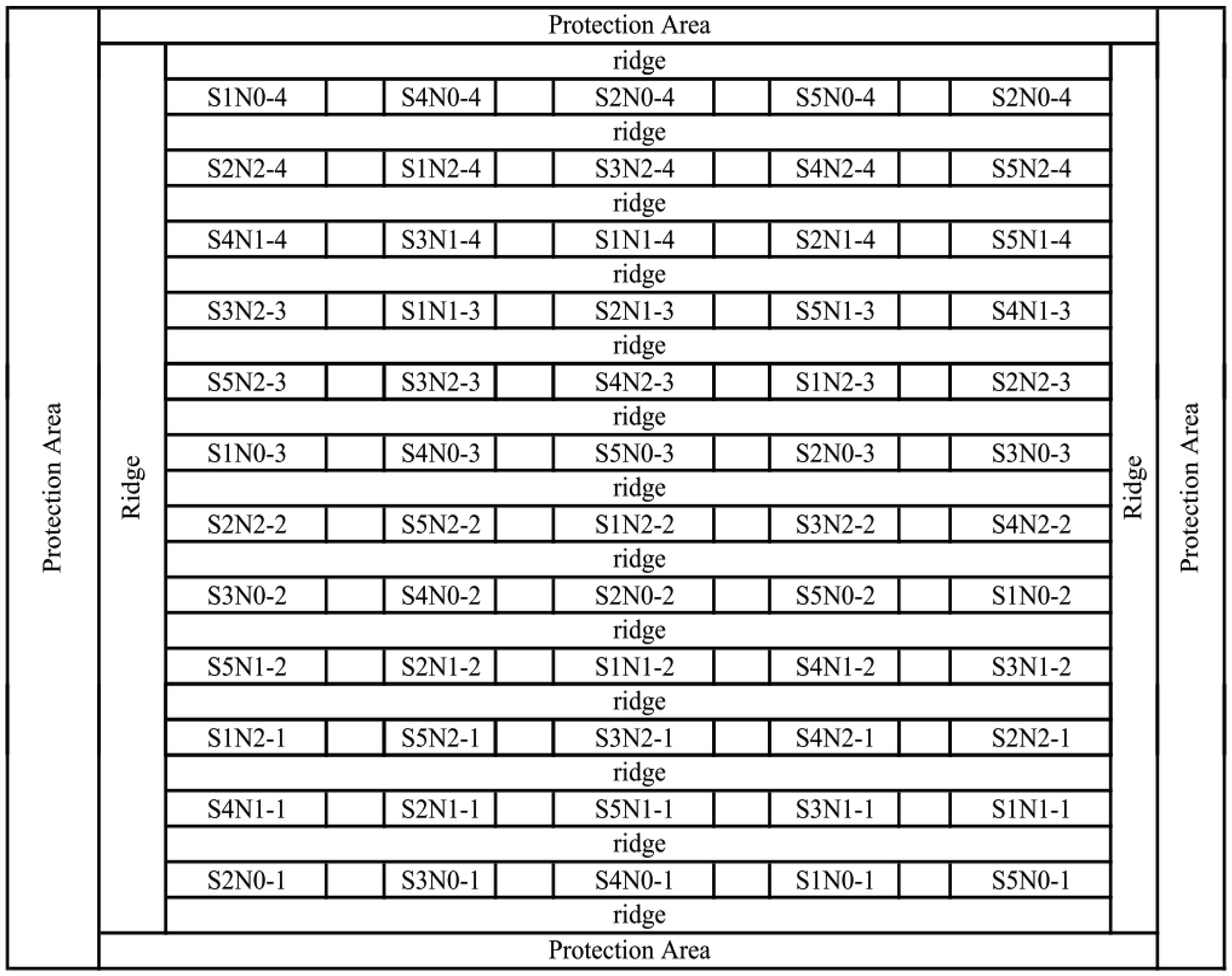
In 2002, the experiment field comprised 60 plots in which different rice cultivars (xiushui 110, Jiayu 293, Jiazao 312, Z00324 and Xieyou 9308) were sown on 2 June in a completely randomized block design with four replicates (Figure 1). The Xieyou 9308 cultivar was a hybrid rice, whereas the others were common rice. Jiayu 293, Jiazao 312, Z00324 and Xieyou 9308 were indicia rice, and Xiushui 110 was japomica rice. The three different levels of N fertilization including no fertilizer (0 kg·ha−1), a normal application rate (120 kg·ha−1), and a superabundant dose of urea (240 kg·ha−1)were applied in the proportions of 45% base fertilizer, 35% tillering fertilizer, and 20% heading fertilizer for each cultivar. In addition, 533.3 kg of Ca(H2PO4)2 ha−1 was applied as a base fertilizer with 300 kg of KCl ha−1 as a heading fertilizer.
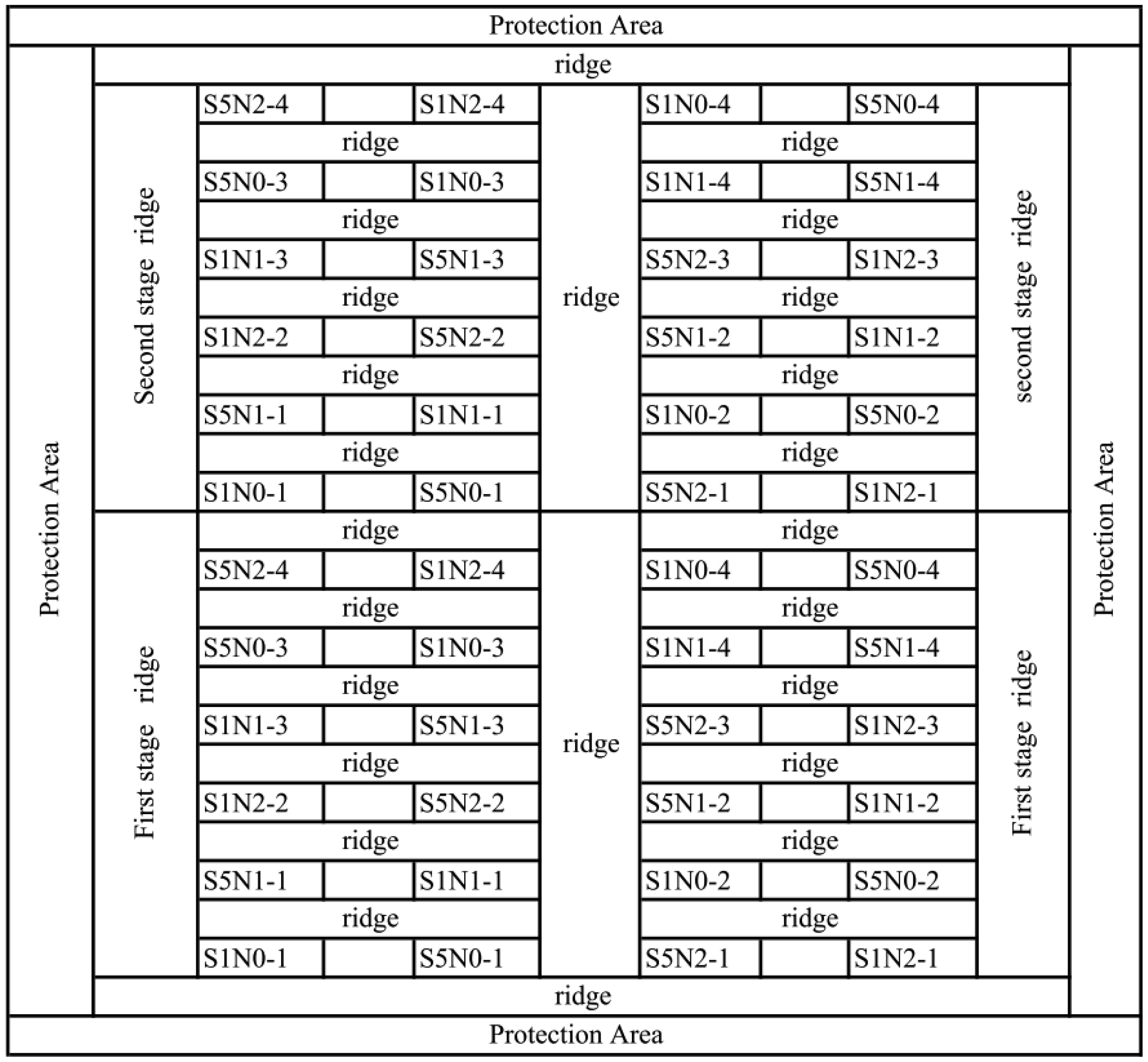
In 2004, the experiment field was consisted of 48 plots of size 4.6 m × 5.46 m. One half of the plots were used for the first experiment and the remaining plots were used for the second experiment (Figure 2). Each experiment involved four replicates of two rice cultivars (xiushui 110 and Xieyou 9308), and the plant density was 45 plants m−2. The first experiment was seeded on 30 May 2004 and the second experiment was seeded on 15 June 2004. Both seedling sets were transplanted to the field one month later. Nitrogen levels and all treatments were identical to the 2002 experiment.
2.2. Canopy Reflectance Measurement
Canopy reflectance measurements were performed under clear-sky conditions at approximately midday (10:00–14:00 LST) using an Analytical Spectral Devices Full Range Spectroradiometer (FieldSpec-FR, ASD, Boulder, CO, USA) during the growing stage, including the early tillering stage, peak tillering stage, gestation stage, heading stage, milky stage and ripening stage. The spectral range and the field of view of the sensor were 350–2,500 nm and 25°, respectively. The sampling interval over the 350–1,000 nm range is 1.4 nm with a resolution of 3 nm, and over the 1,000–2,500 nm range the sampling interval is about 2 nm and the spectral resolution is 10 nm. Fieldspec can acquire both radiance and reflectance data. The reflectance factor of the target is automatically calculated by the instrument as the ratio between the incident radiation, reflected from the surface target, and the incident radiation reflected by a BaSO4 white reference, which is regarded as a Lambertian reflector (the reflectance factor will be called ‘reflectance’ throughout the whole present manuscript. Reflectance spectra were collected from a distance of 1.0 m vertically above the canopies with a field of view of 25°. A single reflectance measurement was obtained as the average of 10 scans to minimize instrumental noise.
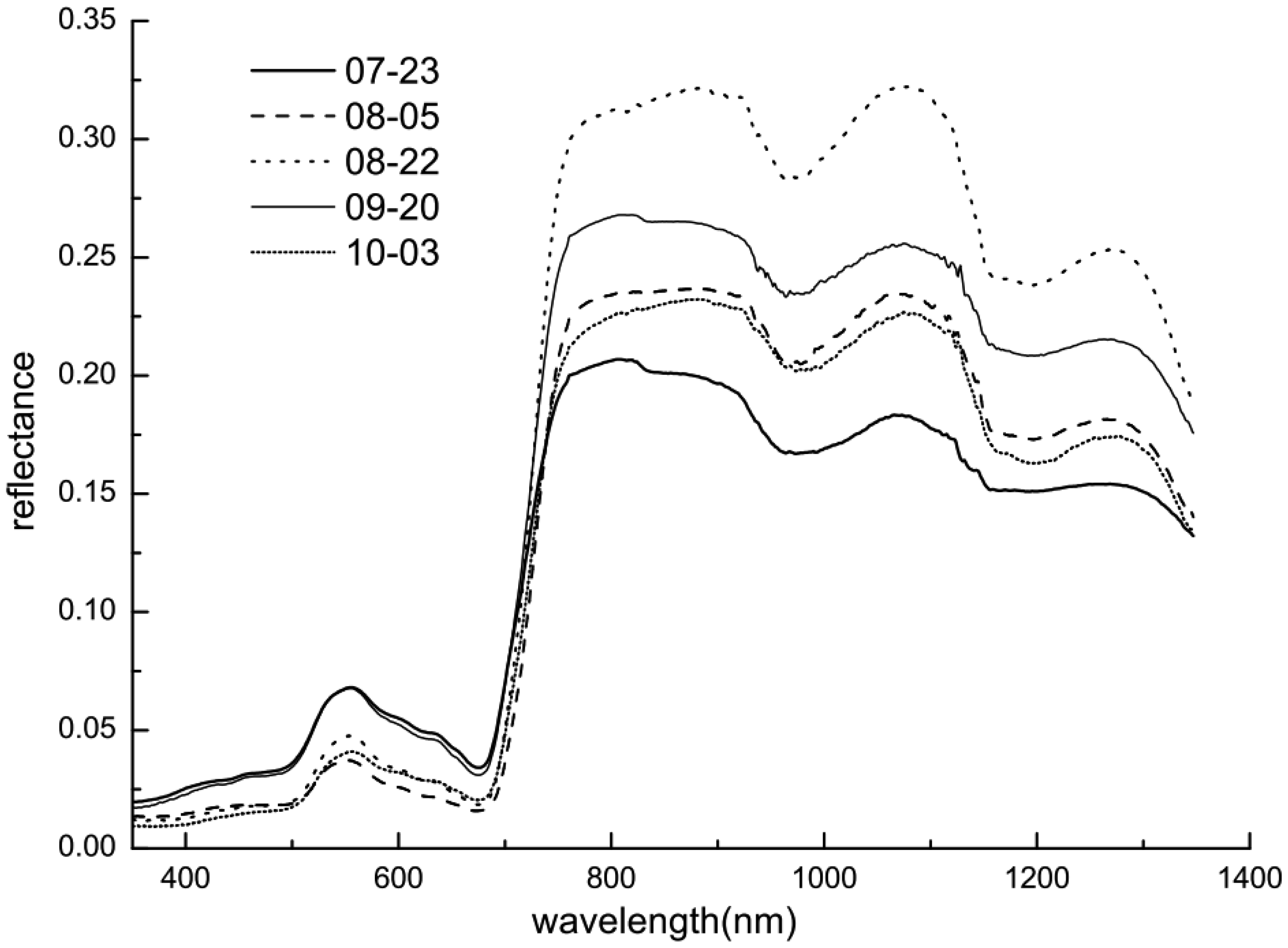
In 2002 spectra were collected on eight dates at distinctive growth stages (17, 23, 30 July, 5, 22, 31 August, 20 September and 3 October) for all experimental field plots. In 2004 measurements were acquired using the same scheme described above on six dates (20 July, 8, 28 August, 22 September and 5, 24 October) during the rice growth stages. For example, the spectral reflectances of the rice canopy at the N1 level of N fertilization at different growth stages in 2002 are shown in Figure 3. As expected, the reflectance spectra of the canopy were significantly different among the various growth stages.
2.3. Satellite Sensors and Their Relative Spectral Response Functions
This study included the evaluation of both high and very high spatial resolution multispectral satellite sensors. Satellite images acquired from these sensors are often used for the detection of vegetation dynamics. Table 1 shows the spectral and spatial characteristics of the satellites sensors used in this study.
The spectral characteristics of the sensor could be characterized by the relative spectral response function (SRF) for each band, which is defined as the ratio of the output signal to the incident flux as a function of wavelength, normalized to the peak value of unity [60]. The SRF indicates the relative sensitivity of a sensor to incoming energy at each wavelength. The relative spectral response function can be described by three key factors, i.e., the center wavelength (CWL), the full width at half the maximum (FWHM), and the shape. The entire set of band SRFs determines the spectral performance of the radiance data. The FWHM, also called bandwidth, indicates the spectral resolution capability of the detector. The SRF shape varies depending on the manner that the sensor disperses and detects the incident light. Sensor models characterize the process converting the spectral response of the land surface-atmosphere system into digital numbers, and the SRF is one of the most important components of sensor modeling system [61].
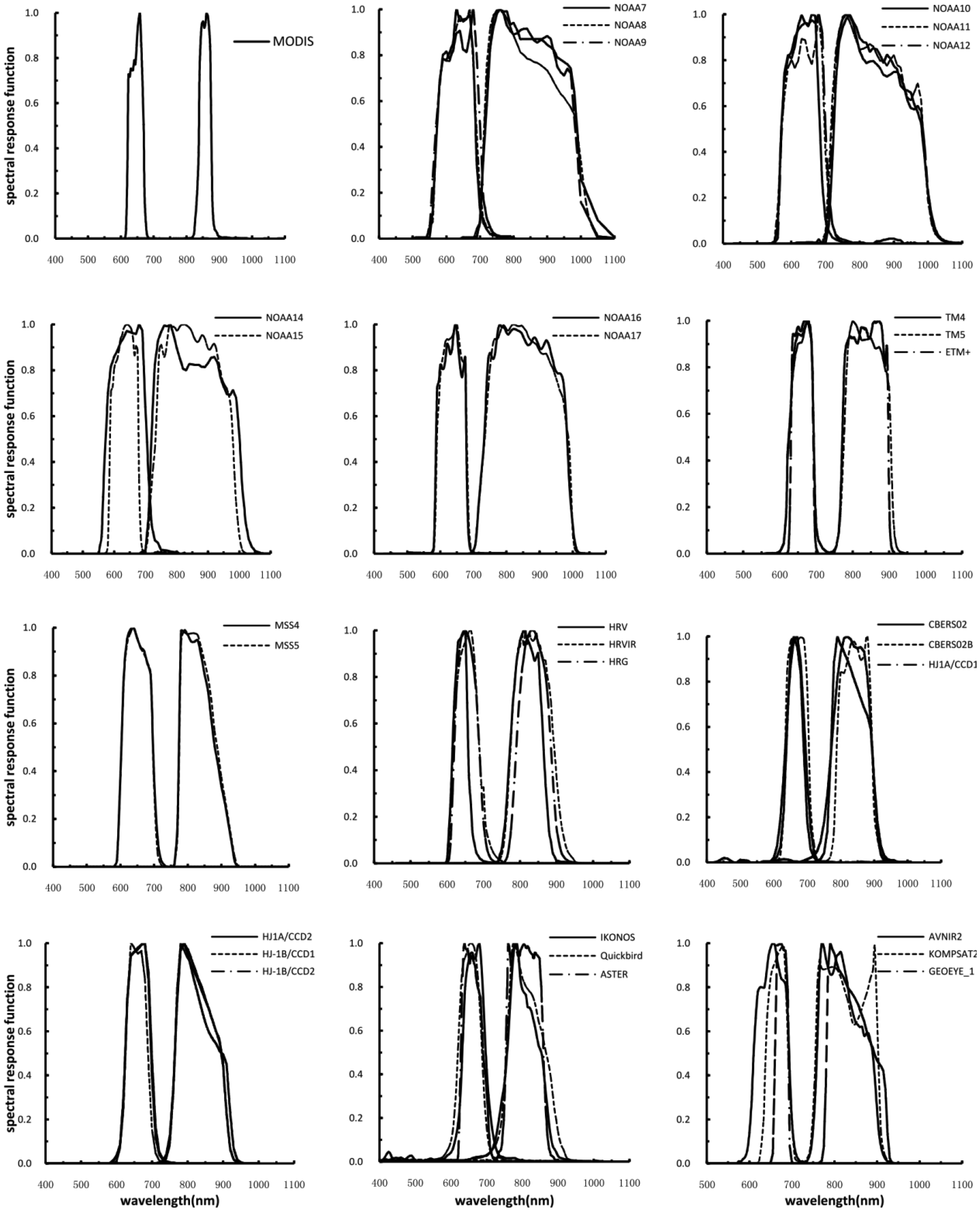
The relative spectral response functions of the red and NIR channels for the different sensors used in this study are shown in Figure 4 and Table 1. These sensors include NOAA7-17AVHRRs, SPOT HRV, Landsat TMs, ETM+, MSS, HJ1A/B CCDs, CBERS CCDs, IKONOS, QuickBird, and ALOS AVNIR2. The SRFs were obtained from the operator's website or by personal communication. Though similar, these curves differ in their shape, central wavelength location, bandwidth, and degree of overlap between channels, especially with respect to the transition from the chlorophyll absorption band to the foliage reflection band (0.68–0.72 μm). The spectral response functions of the sensors vary from one another, especially in the NIR region.
A comparison of the spectrally matched bands between MODIS and other sensors indicated that the spectral ranges of the MODIS red and NIR channels are much narrower than those for the other sensors and have no overlap with each other over the vegetation transition band (Figure 4). It was clearly evident that the gap between the red and NIR band of MODIS was wider than the gap between the red and NIR band of the other sensors, even where an overlap exists. Thus, the other sensor bands are closer to the red edge relative to MODIS. It was noted that the Landsat TMs, SPOT HRVs and NOAA AVHRRs response curves varied depending on the version of the instrument that was employed. The bandwidths of the Landsat7 ETM+ channels are narrower than those of TM on Landsat4 and 5. A similar result was also found for the new instrument AVHRR3 onboard NOAA15, 16 and 17. The channels of the new AVHRR3 instrument have narrower bandwidths and a much smaller overlap over the vegetation transition band than do the other AVHRRs. This indicated that a direct comparison of spectral reflectance or vegetation indices produced by various sensors should be performed with caution.
2.4. Bandpass Target Reflectance Simulation
Some sensor simulation methods take into account both the spectral and spatial differences of the sensor [62]. In this study, our objective was to assess the spectral band differences solely caused by different spectral response functions without considering atmospheric intervention. Moreover, the only variation in the simulation based on the same spectra was the spectral response function of the sensor, and this is the only parameter that enables us to compare the different sensors.
To simulate the multiple bands from hyperspectral bands, the reflectance of the narrow hyperspectral bands must be convoluted with the spectral response function of each band that simulates the bands of the satellite sensors. Prior to simulation, each hyperspectral central wavelength was linked with the mean SRF value (in the range of the full width half maximum (FWHM) of the hyperspectral band) of the simulated band. This approach was similar to the method proposed by Franke et al. [63]. The equation for simulating the reflectance of the sensor can be expressed as follows:
The normalized difference vegetation index was then calculated as follows:
2.5. Comparison of Reflectance and NDVI between MODIS and Other Sensors
A comparative analysis of the red/near-infrared reflectance and NDVI for various sensors was performed using two statistical measurements namely, the relative percentage difference (RPD) and absolute percentage difference (APD). The computations were conducted for different sensors with the MODIS sensor as a reference, and the following formula was used to compute the RPD and APD:
However, it was not clear whether the differences in the reflectance and NDVI between MODIS and the other sensors were statistically significant. Thus, a paired Student t test was used to compare the differences in the reflectance and NDVI between MODIS and the other sensors in this study.
3. Results and Discussion
The simulated reflectances for the 31 different satellite sensors were calculated to quantify the influence of the varying spectral response functions on the target reflectance in the red band, NIR band and NDVI. The effects of the SRF on the reflectance in the red and NIR channels and NDVI were then evaluated based on RPD and APD with respect to the MODIS values.
3.1. The Effect of the SRF on the Reflectance in the Red Channel
The minimum, maximum and mean values as well as the standard deviation of the red reflectance for various satellite sensors simulated using paddy rice canopy reflectance data are listed in Table 2. For Terra-MODIS, the simulated reflectance in the red channel ranged from 0.0128 to 0.1337, and the mean reflectance value was 0.0354. In this study, we used this instrument as a reference due to its high spatial and temporal coverage. The largest mean reflectance in the red was found for IKONOS at 0.0460, followed by the AVHRR2 onboard NOAA12 (0.0454), NOAA14 (0.0453) and NOAA11 (0.0441). The lowest mean reflectance was observed for GEOEYE-1 at 0.0313, followed by Landsat7-ETM+ (0.0336), KOMPAST2 (0.0343) and MODIS (0.0354).
The RPDs for all other sensors in this study in the red band with respect to MODIS were between −21.02% and 77.73% (Table 2). The mean RPD between MODIS and various other sensors, averaged over 447 samples, ranged from −12.67% (GEOEYE-1) to 36.30% (IKONOS). Similar to GEOEYE-1, Landsat7 ETM+ and KOMPSAT2 showed negative RPDs of −5.6% and −3.58%, respectively. The comparison indicated that the red reflectances of GEOEYE-1, Landsat7 ETM+ and KOMPSAT2 were smaller than that of MODIS. With the exception of the above three sensors, the red reflectances of the other sensors were larger than that of MODIS. It was observed that AVHRR2 onboard NOAA7, 9, 11, 14, and 12 (20.66%, 27.96%, 29.04%, 32.98%, 33.84%, respectively) had a higher mean RPD with respect to MODIS than did AVHRR1 and AVHRR3 onboard NOAA8 and 10 (18.11% and 17.10%, respectively) and NOAA15, 16, 17(10.93%, 9.07%, and 5.99%, respectively). The mean RPD for Landsat4 TM, Landsat5 TM, SPOT1 HRV, SPOT4 HRVIR and SPOT5 HTG were 1.11%, 0.95%, 6.10%, 14.13% and 3.75%, respectively. The mean RPD for CCD1 onboard HJ1-A and HJ1-B were 6.27% and 2.81%, respectively, whereas the values for CCD2 onboard HJ1-A and HJ1-B were 13.25% and 11.27%, respectively. The ASTER and ALOS AVNIR2 sensors having a high spatial resolution showed small RPDs of 3.91% and 4.25%, respectively, as compared to QuickBird and IKONOS.
The minimum APD between MODIS and the other sensors was observed for Landsat5 TM with a value of 0.0013%, and the maximum APD was observed for IKONOS with a value of 77.73%. The smaller difference was identified for Landsat5-TM with a mean APD value of 1.28%, followed by Landsat4-TM (1.36%), HJ-1B(CCD1) (2.85%) and KOMPSAT2(3.62%). The largest difference was observed for IKONOS with a mean APD value of 36.30%, followed by AVHRR2 onboard NOAA12 (33.84%), 14 (32.98%) and 11 (29.04%). AVHRR2 onboard NOAA7, 9, 11, 14, and 12 had higher mean APD with respect to MODIS than did the AVHRR1 and AVHRR3 onboard NOAA8, 10 and NOAA15, 16, 17. With the exception of Landsat5 TM, Landsat4 TM, HJ-1B CCD1, KOMPSAT2, Terra ASTER and Landsat7 ETM+, the mean APD value of the other sensors were equivalent to the RPD with respect to MODIS (Table 2).
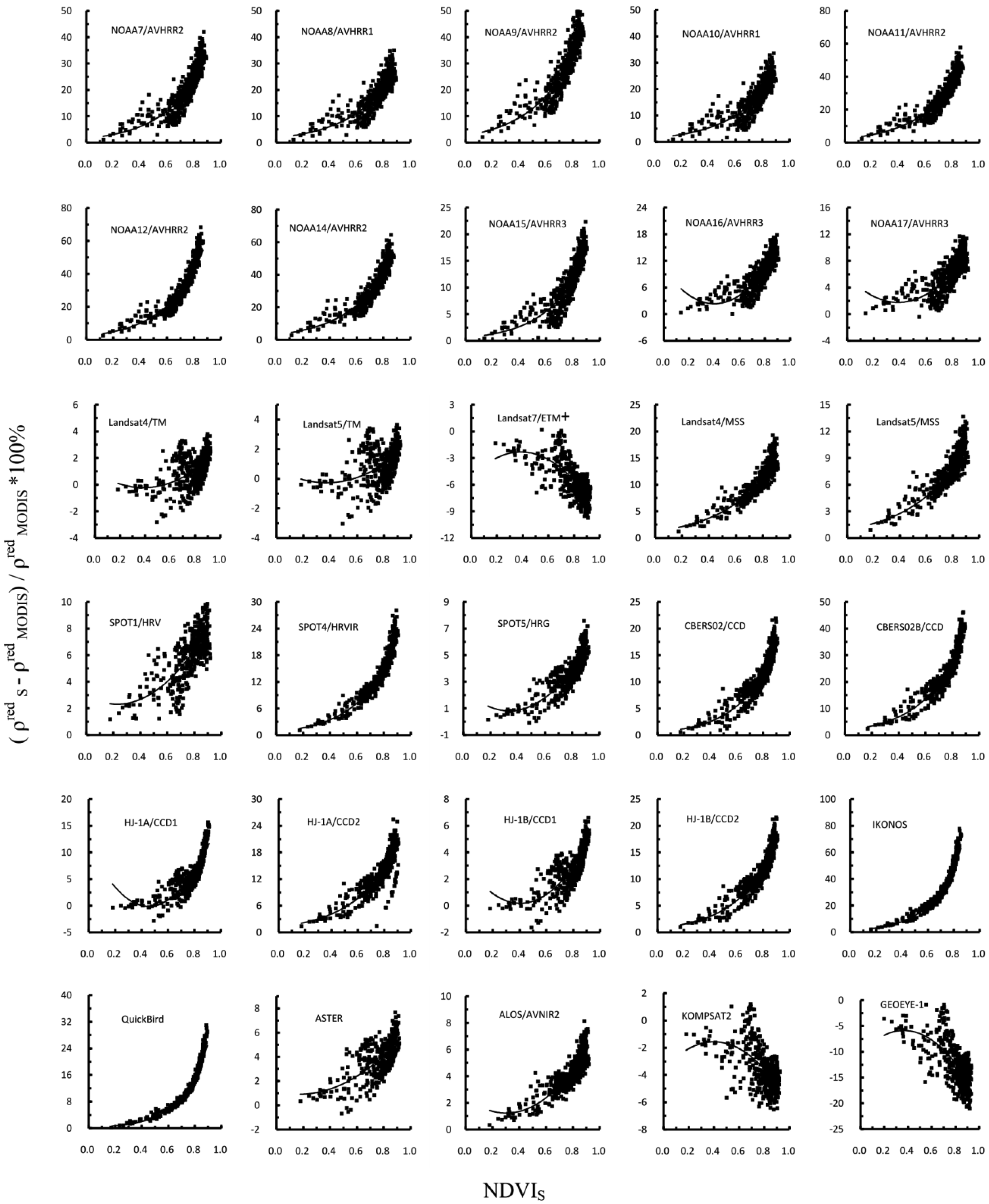
Further analysis of the significance based on paired t tests indicated that the differences in the red reflectance between MODIS and the other sensors were highly significant (p < 0.0001). The analysis of difference indicated that it is important to apply the spectral correction when using combined data from MODIS and the other sensor. The discrepancies caused by different SRFs may be corrected using the second-degree polynomial functions and exponential functions, as shown in Figure 5. The curves were produced by fitting the data points. Figure 5 shows that the RPD in the red reflectance for all other sensors in this study increased with increasing target NDVI values, excluding KOMPSAT2, Landsat7 ETM+ and GEOEYE-1. The value of the mean absolute difference for KOMPSAT2, Landsat7 ETM+ and GEOEYE-1 was negative. Thus, the direction of the curves for these three sensors was opposite that of the other sensors. The coefficients of the quadratic and exponential functions that best fit the data and correlation coefficient of the fit for each sensor for the red reflectance are shown in Table 3. The quality of the fit was high for AVHRRs, IKONOS and CBERS02B CCD, whereas data for the TM and ASTER sensors were more scattered.
3.2. The Effect of the SRF on the Reflectance in the NIR Channel
The descriptive statistics of the NIR reflectances for various satellite sensors simulated using paddy rice canopy reflectance are listed in Table 4. For Terra MODIS, the simulated reflectance in the NIR channel ranged from 0.0927 to 0.5023, and the mean reflectance value was 0.3019. The highest mean reflectance value in the NIR channel was 0.3019 for MODIS, followed by SPOT5 HRG (0.3008), CBERS02B CCD (0.3006) and GEOEYE-1 (0.3005). The lowest mean reflectance was observed for NOAA8 AVHRR1 with a value of 0.2757, followed by IKONOS (0.2782), AVHRR2 onboard NOAA-11 (0.2784) and NOAA-9 (0.2787).
Among the studied sensors, the minimum RPD with respect to MODIS in the NIR band was −12.29% for NOAA14 AVHRR2, and the maximum RPDs was 56.94% for SPOT5 HRG. The mean RPD of the NIR reflectance varied from −8.52% (NOAA8 AVHRR1) to −0.23% (SPOT5 HRG). The mean RPD for all of the sensors with respect to MODIS was negative. The mean RPD was within −7.66% to −6.93%, −5.15% to −4.98%, −1.20% to −1.06% and −0.47% to −0.40% for the AVHRR2s, AVHRR3s, HJ-1A/B CCDs and Landsat TMs sensors, respectively. The mean RPDs for SPOT1 HRV, SPOT4 HRVIR and SPOT5 HRG were −0.99%, −0.57% and −0.23%, respectively.
The largest mean APD in the NIR channel was observed for NOAA8 AVHRR1 with a value of 8.71%, followed by AVHRR2 onboard NOAA11 (7.86%), NOAA9 (7.76%) and IKONOS (7.69%). For the AVHRR2 instruments, the mean APDs ranged from 7.14% to 7.86%. AVHRR3 had a little smaller APD than did AVHRR1s and AVHRR2s at 5.19%, 5.30% and 5.36% for NOAA17, NOAA15 and NOAA16, respectively. The smallest difference was identified for CBERS02B CCD with the mean APD value of 0.84%, followed by GEOEYE-1 (0.91%), SPOT5 HRG (0.94%) and Landsat4-TM (0.98%). The mean APD for Landsat TMs, MSSs, and SPOT4 HRVIR ranged from 0.98% to 1.20%, whereas the values ranged from 1.62% to 1.70% for the HJ CCDs.
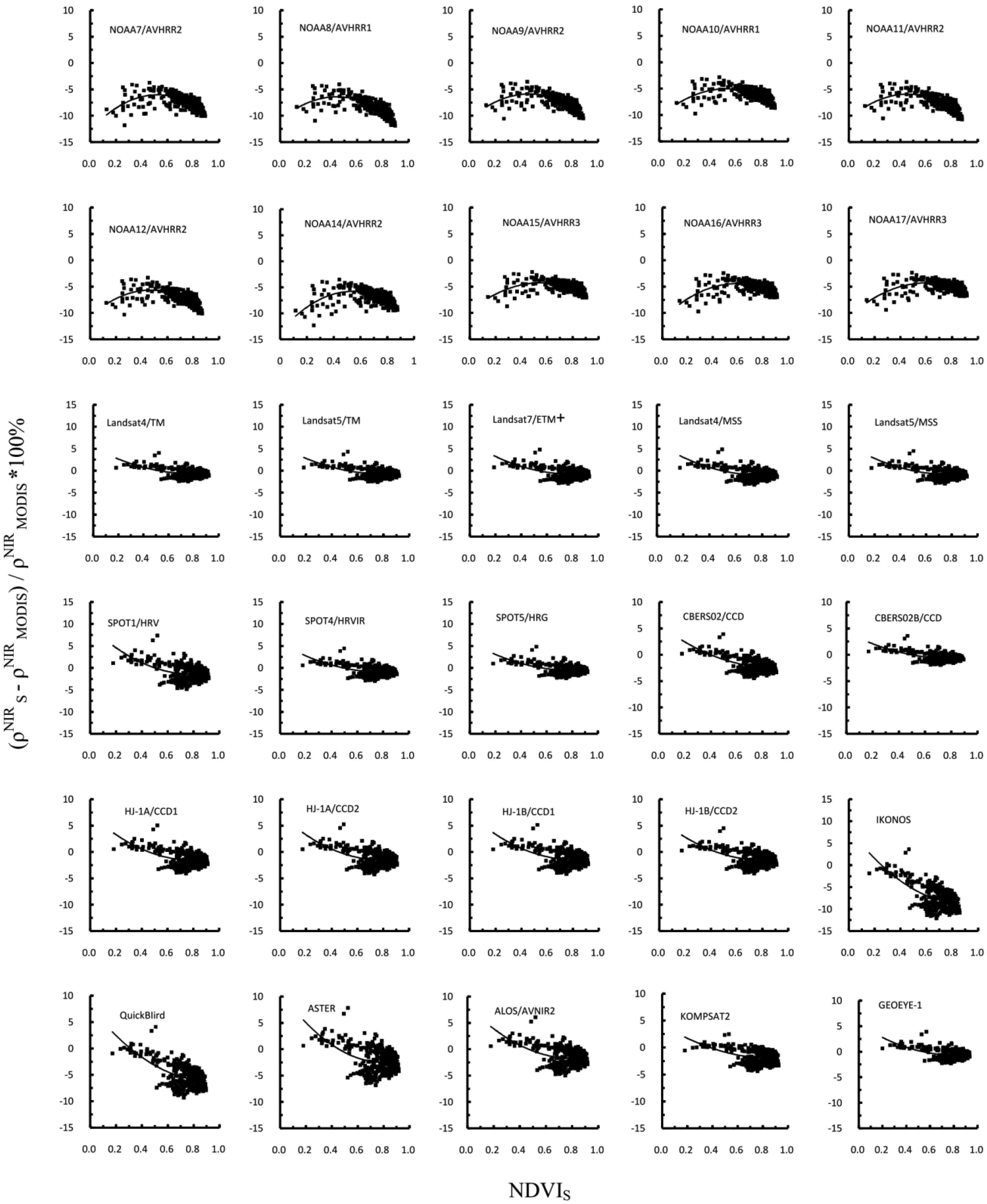
The analysis using paired t tests indicated that the differences in the NIR reflectance between MODIS and other sensors were significant at the p < 0.0001 level. The discrepancies caused by different SRFs may be corrected using second-degree polynomial functions, as shown in Figure 6 and Table 5.
These curves were produced by fitting the data points. The RPDs for AVHRRs onboard NOAA7-17 showed two distinct trends with increasing target NDVI values. Specifically, the difference increased as the target NDVI value increased from 0 to 0.5; however, as the target sensor NDVI value increased above 0.5, the RPD began to decrease. The observed trends in the NIR reflectance differences are likely due to the inclusion of either the red edge or leaf liquid water absorption regions in the broad bandpass of AVHRR channel 2. The coefficients of the quadratic functions that best fit the data and correlation coefficient of the fit for each sensor for NIR reflectance were given in Table 5. The quality of the fits was higher for AVHRRs, IKONOS and QuickBird than other sensors.
3.3. The Effect of the SRF on the NDVI
Table 6 showed the minimum, maximum and mean values as well as the standard deviation of the NDVI for various satellite sensors. For Terra MODIS, the NDVI ranged from 0.177 to 0.9237, and the mean NDVI value was 0.7756. The lowest mean NDVI was observed for KONOS at 0.7043, followed by the AVHRR2 onboard NOAA12 (0.7071), 14 (0.7081), and 11 (0.7131). The largest mean reflectance was observed for GEOEYE-1 at 0.7973, followed by Landsat7 ETM+ (0.7845), KOMPAST2 (0.7788) and MODIS (0.7756).
Table 6 showed that the RPDs in the NDVI for all studied sensors range from −35.24% to 14.16%. IKONOS showed the lowest mean RPD of −9.32% with respect to MODIS. Similar to IKONOS, AVHRR2 onboard NOAA12, 14, 11, 9 and 7 had RPDs of −9.29%, −9.29%, −8.56%, −8.37%, and −6.72%, respectively. However, AVHRR1 onboard NOAA8 and 10 and AVHRR3 onboard NOAA15, 16, and 17 showed slightly higher mean RPDs of −6.56%, −5.61%, −3.85%, −3.57%, and −2.87%, respectively. The largest mean RPD was observed for GEOEYE-1 at 3.10%, followed by Landsat7 ETM+ (1.28%), KOMPSAT2 (0.48%), Landsat5 TM (−0.18%) and Landsat4 TM (−0.21%). The mean RPDs for SPOT1 HRV, SPOT4 HRVIR and SPOT5 HTG were −1.55%, −3.0% and 0.77%, respectively. The mean RPD for CCD1 onboard HJ1-A and HJ1-B was −1.37% and −0.72%, respectively, whereas the values for CCD2 onboard HJ1-A and HJ1-B were −3.07% and −2.62%, respectively. The sensors having a high spatial resolution, such as ASTER and ALOS AVNIR2, showed larger RPDs of −1.24% and −1.16%, respectively.
The minimum mean APD in the NDVI between MODIS and the other sensors was observed for Landsat4 TM with a value of 0.59%, followed by Landsat5 TM (0.60%), KOMPSAT2(0.75%) and SPOT HRG (0.92%). The mean APDs were 1.27%, 1.34%, 1.43%, 1.59%, 1.62% and 1.82% for ALOS AVNIR2, LANDSAT7 ETM+, Terra ASTER, HJ-1A CCD, SPOT1 HRV and LANDSAT5 MSS, respectively. Compared to Landsat5 MSS and HJ-1A CCD1, the mean APD was 2.47%, 2.64% and 3.09% for LANDSAT4 MSS, HJ-1B CCD2 and HJ-1A CCD2, respectively. The maximum mean APD between MODIS and the other sensors was observed for IKONOS with a value of 9.32%, followed by AVHRR2 onboard NOAA12 (9.29%), NOAA 14 (9.29%) and NOAA 11 (8.56%). AVHRR2 onboard NOAA7, 9, 11, 14, and 12 showed higher mean APDs with respect to MODIS than did the AVHRR1 and AVHRR3 onboard NOAA8 and 10 (6.57% and 5.62%) and NOAA15, 16, 17 (3.87%, 3.59%, and 2.89%).
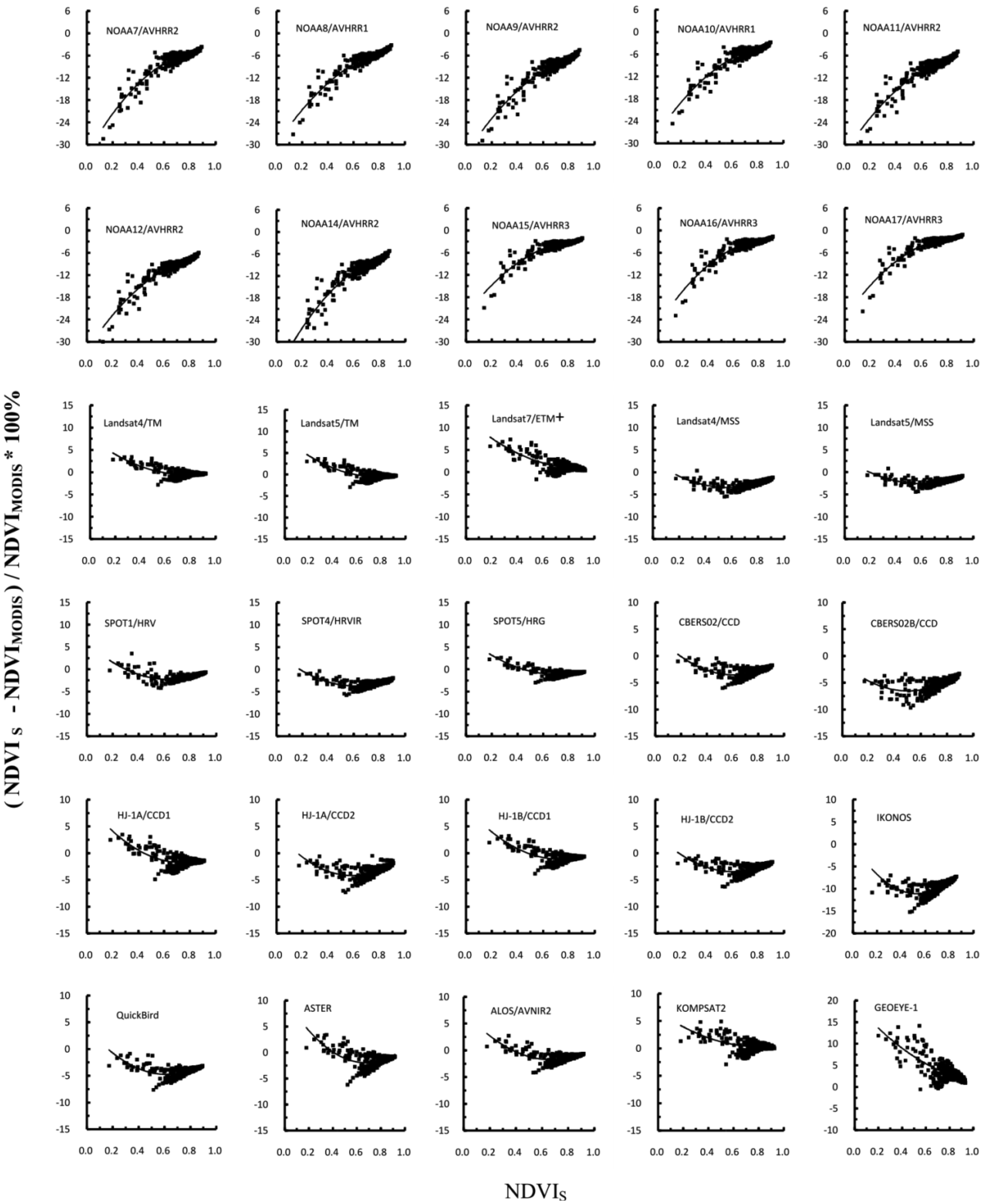
The paired t tests confirmed that there were significant differences (p < 0.0001) in NDVI between MODIS and the other sensors. The discrepancies caused by different SRFs may be corrected using second-degree polynomial functions, as shown in Figure 7. The curves were produced by fitting the data points. It was observed that the RPDs in the NDVI with respect to MODIS for AVHRRs increased with increasing target NDVI values. The coefficients of the quadratic functions that best fit the data, as well as the correlation coefficient of the fit for each sensor for the NDVI, are provided in Table 7. The quality of the fit was high for the AVHRRs, whereas the data for the KOMPSAT2 sensors were more scattered.
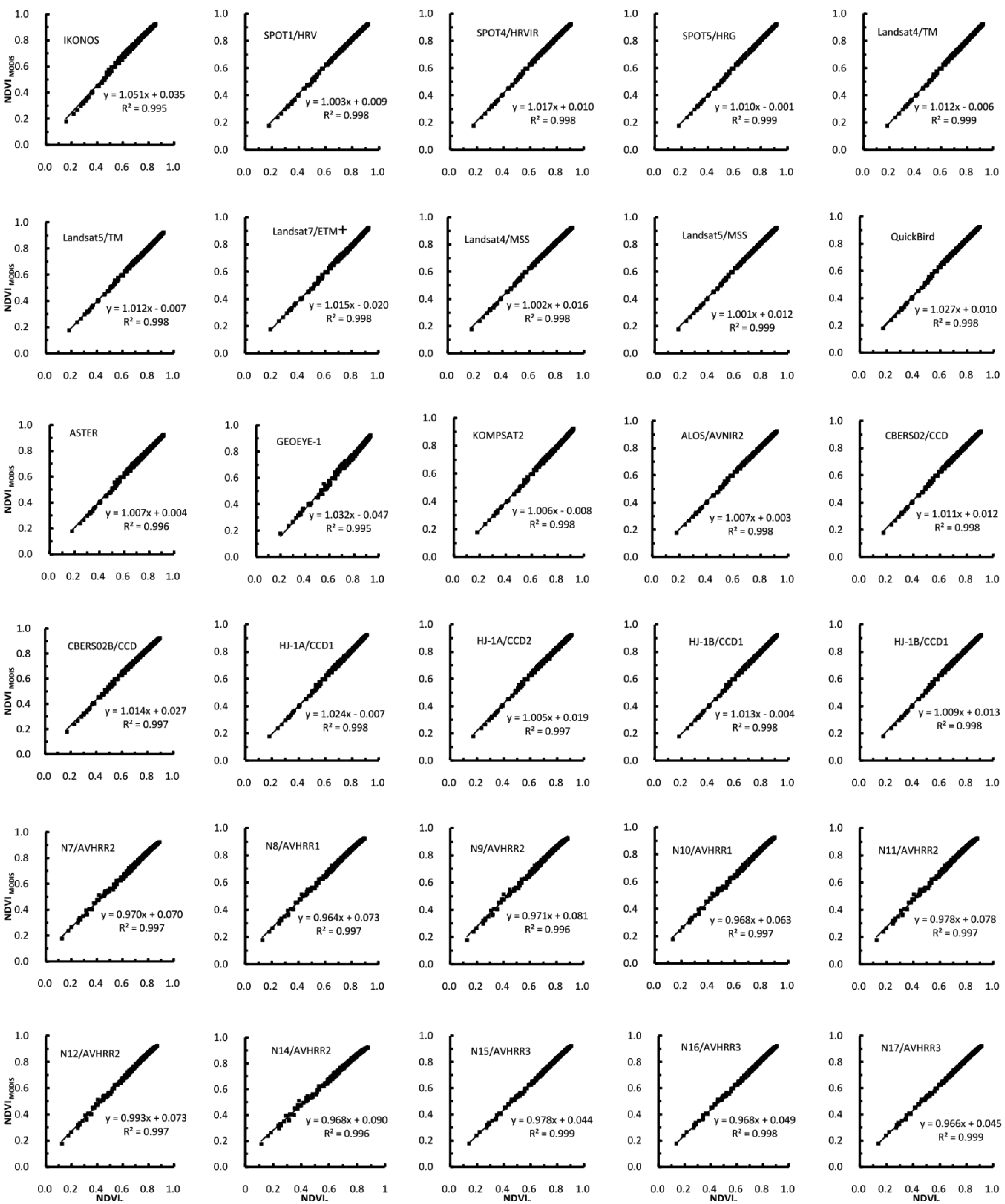
A comparison of the NDVIs simulated for different sensors showed that the relationship between MODIS and other the instrument NDVI values can be evaluated using a linear regression model (Figure 8). The linear regression relationships between the NDVI values of the various sensor combinations presented in Figure 8 were all significant at p < 0.0001. Additionally, the coefficient of determination was higher than 0.99 in almost every case. However, the relationships were not 1:1. The intercept values for all sensors ranged from −0.047 (GEOEYE-1) to 0.090 (NOAA14). The slope values varied from 0.965 (NOAA8) to 1.051 (IKONOS), and the r2 values varied from 0.995 (IKONOS) to 0.999 (SPOT5/HRV). The results showed substantial differences between the sensor systems, which if uncorrected, would significantly bias the estimates of any biophysical parameters derived from these sensors. Even for a nominally continuous system, the NDVIs from the Landsat-ETM+ sensor differed from the values from the earlier TM sensor; therefore, the relationship between MODIS and each sensor varies. The results indicated that the relationships between the NDVIs were sufficiently robust in all cases to allow for corrections between one system relative to MODIS.
3.4. Comparison with Previous Studies
The results of the current study were consistent with the previous research by Trishchenko et al. [53]. The study investigated the effect of the SRF on reflectance and NDVI of the moderate resolution satellite sensors, including MODIS and AVHRRs. They found differences in the red band reflectance between MODIS and other sensors were relatively higher than that in the NIR band reflectance. This phenomenon of higher relative red band differences was observed in this study. In addition, the findings of comparison of MODIS and AVHRR NDVI data included in our study were identical with other studies. The MODIS NDVI data were found to be greater than the AVHRR NDVI data in an analysis over Senegal [64], South Florida [65], the Southern Great Plains of the United States [53] and simulation of MODIS and AVHRR data [48].
Our results also agreed well with the findings of other studies [30,46,48] related to the NDVI cross-sensor correction. The simulations by Steven et al. [48] were based on measurements of a full range of sugar beet and maize canopies. Whereas the study by van and Gonsamo et al. [30,46] included large sets of measured backgrounds as input to radiative transfer models (i.e., SAIL, PROSPECT and 6S) to simulate canopy spectra for a large range of possible global vegetation conditions. They used simple linear regression models for cross-sensor correction. The slope and intercept values of the linear regression relationships between the NDVI values of the various sensor combinations for SPOT, MSS, TM, ETM+, IKONOS and QuickBird with an MODIS reference were almost identical to those in the present study.
This study indicated that reflectance and NDVI derived from different sensors cannot be considered as directly equivalent and NDVI based on surface reflectance can be corrected for spectral band effects. Our study was based on simulating the spectral band responses of different satellite sensors from field reflectance data. The advantages of this method are that the results are not affected to any extent by calibration errors or atmospheric interactions and the simulations can be performed for any combination of sensors for direct comparisons. However, it should be noted that other instrumental effects, such as spatial sampling and the radiometric resolution, and atmospheric corrections are not accounted for by this approach. Miura concluded that the MODIS versus AVHRR3 and AVHRR2 cross-sensor NDVI relationships were subject to larger difference due to the NIR bands which showed differential sensitivities to the atmospheric water vapor effects between sensors [66]. Therefore, accurate calibrations and atmospheric corrections are also essential for combination of data from different satellite systems.
4. Conclusions
Long-term monitoring of the Earth's environment using multi-source satellite sensors requires consistent and comparable measurements. However, the combined use of the multi-source satellite data sets requires a detailed evaluation of their compatibility and consistency to avoid artifacts. In this study, rice canopy spectra were collected from field experiments so as to quantify the effect of the sensor spectral response function on the red and NIR reflectances and NDVI derived from 31 Earth observation satellite sensors, including CBERS CCD and HJ1-A/B CCD. This study not only included sensors having a coarse spatial resolution, such as AVHRRs from NOAA-7 to NOAA-17 and MODIS, but also included sensors having a medium spatial resolution, such as Landsat TMs and MSSs, SPOT HRV, HRVIR and HRG, CBERS CCDs, and HJ CCDs. Moreover, we also showed sensors having a relatively high spatial resolution, such as IKONOS, QuickBird, KOMPSAT2 and GEOEYE-1. All of the sensors were compared to the Terra MODIS, which was chosen as a reference. Based on field reflectance data, we simulated the spectral band responses of different satellite sensors.
The results showed that the mean RPD in the red reflectance for all other sensors with respect to MODIS ranged from −12.67% (GEOEYE-1) to 36.30% (IKONOS). For GEOEYE-1, Landsat7 ETM+ and KOMPSAT2, the negative RPD indicated that red reflectance of MODIS was larger than that of these sensors. The mean APD in red reflectance varied from 1.28% (Landsat5-TM) to 36.30% (IKONOS). AVHRR2 onboard NOAA7, 9, 11, 14, and 12 showed a higher mean APD with respect to MODIS than the AVHRR1 and AVHRR3 onboard NOAA8 and 10 (18.11% and 17.10) and NOAA15, 16, and 17(10.93%, 9.07%, and 5.99%).
The mean RPD in the NIR reflectance for all other sensors with respect to MODIS ranged from −8.52% (NOAA8 AVHRR1) to −0.23% (SPOT5 HRG). It was observed that the mean RPD for all sensors with respect to MODIS was negative. The mean RPD ranged from −7.66% to −6.93%, −5.15% to −4.98%, −1.20% to −1.06% and −0.47% to −0.40% for the AVHRR2s, AVHRR3s, HJ CCDs and Landsat TMs, respectively. The largest mean APD was observed for NOAA8 AVHRR1 at 8.71%, and the smallest difference was observed for CBERS02B CCD at 0.84%. For the AVHRR2 instruments, the mean APDs were within the range of 7.14% to 7.86%. The AVHRR3 showed slightly smaller APD than did AVHRR1s and AVHRR2s, which were 5.19%, 5.30% and 5.36% for NOAA17, 15, and 16, respectively. The mean APD for the Landsat TMs, MSSs, and SPOT4 HRVIR was 0.98% to 1.20% and was 1.62% to 1.70% for the HJ CCDs.
With respect to MODIS, the mean RPDs in the NDVI for all sensors in this study ranged from −9.32% to 3.10%. The mean APDs in the NDVI varied from 0.59% (Landsat5-TM) to 9.32% (IKONOS). The mean APD was 1.27%, 1.34%, 1.43%, 1.59%, 1.62% and 1.82% for ALOS AVNIR2, Landsat7 ETM+, Terra ASTER, HJ-1A CCD, SPOT1 HRV and LANDSAT5 MSS, respectively. Comparison with Landsat5 MSS and HJ-1A CCD1, the mean APD was 2.47%, 2.64%, 3.09% for LANDSAT5 MSS, HJ-1B CCD2 and HJ-1A CCD2. AVHRR2 onboard NOAA7, 9, 11, 14, 12 has higher mean APD with respective to MODIS than the AVHRR1 and AVHRR3 onboard NOAA8, 10 (6.57%, 5.62%) and NOAA15, 16, and 17 (3.87%, 3.59%, and 2.89%).
The results of paired t tests showed that there were significant differences (p < 0.0001) between MODIS and all the other sensors regarding the red reflectance, NIR reflectance and NDVI. A series of optimum models were provided for spectral corrections between MODIS and other sensors. This result offers improved opportunities for monitoring crops through the growing season and the prospects of better continuity of long-term monitoring of vegetation responses to environmental change.
Acknowledgments
We acknowledge Yanlin Tang, Qian Cheng, Junfeng Xu, Lei Zhu, Zhanyu Liu, Yuan Wang, Qiuxiang Yi, and Yan Jin for their contributions to the spectral measurements of the rice canopy. We thank the anonymous reviewers who provided valuable comments. This work was supported by grants from the National High Technology Research and Development Program of China (2012AA12A30703), the Natural Science Foundation of China (51109183) and the Ph.D. Programs Foundation of the Ministry of Education of China (20100101110035, 20110101120036).
Conflicts of Interest
The authors declare no conflict of interest.
References
- Cracknell, A.P. The exciting and totally unanticipated success of the AVHRR in applications for which it was never intended. Adv. Space Res. 2001, 28, 233–240. [Google Scholar]
- Defries, R.S.; Belward, A.S. Global and regional land cover characterization from satellite data: An introduction to the Special Issue. Int. J. Remote Sens. 2000, 21, 1083–1092. [Google Scholar]
- Tucker, C.J. Red and photographic infrared linear combinations for monitoring vegetation. Remote Sens. Environ. 1979, 8, 127–150. [Google Scholar]
- Tucker, C.J. Remote sensing of leaf water content in the near infrared. Remote Sens. Environ. 1980, 10, 23–32. [Google Scholar]
- Gallo, K.P.; Daughtry, C.S.T.; Bauer, M.E. Spectral estimation of absorbed photosynthetically active radiation in corn canopies. Remote Sens. Environ. 1985, 17, 221–232. [Google Scholar]
- Goward, S.N.; Tucker, C.J.; Dye, D.G. North American vegetation patterns observed with the NOAA-7 advanced very high resolution radiometer. Vegetatio 1985, 64, 3–14. [Google Scholar]
- Wang, Q.; Adiku, S.; Tenhunen, J.; Granier, A. On the relationship of NDVI with leaf area index in a deciduous forest site. Remote Sens. Environ. 2005, 94, 244–255. [Google Scholar]
- Myneni, R.B.; Nemani, R.R.; Running, S.W. Estimation of global leaf area index and absorbed par using radiative transfer models. IEEE Trans. Geosci. Remote Sens. 1997, 35, 1380–1393. [Google Scholar]
- Myneni, R.B.; Williams, D.L. On the relationship between FAPAR and NDVI. Remote Sens. Environ. 1994, 49, 200–211. [Google Scholar]
- Potter, C.S. Terrestrialbiomass and the effects of deforestation on the global carbon cycle—Results from a model of primary production using satellite observations. Bioscience 1999, 49, 769–778. [Google Scholar]
- Schloss, A.L.; Kicklighter, D.W.; Kaduk, J.; Wittenberg, U. Intercomparison, ThE.P.OF.ThE.P.NpP.M. Comparing global models of terrestrial net primary productivity (NPP): Comparison of NPP to climate and the normalized difference vegetation index (NDVI). Glob. Chang. Biol. 1999, 5, 25–34. [Google Scholar]
- Donohue, R.J.; McVicar, T.R.; Roderick, M.L. Climate-related trends in Australian vegetation cover as inferred from satellite observations, 1981–2006. Glob. Chang. Biol. 2009, 15, 1025–1039. [Google Scholar]
- Ichii, K.; Kawabata, A.; Yamaguchi, Y. Global correlation analysis for NDVI and climatic variables and NDVI trends: 1982–1990. Int. J. Remote Sens. 2002, 23, 3873–3878. [Google Scholar]
- McVicar, T.R.; Jupp, D.L. B. The current and potential operational uses of remote sensing to aid decisions on drought exceptional circumstances in Australia: A review. Agr. Syst. 1998, 57, 399–468. [Google Scholar]
- Eklundh, L.; Olsson, L. Vegetation index trends for the African Sahel 1982–1999. Geophys. Res. Lett. 2003, 30, 1430. [Google Scholar]
- Tucker, C.J.; Slayback, D.A.; Pinzon, J.E.; Los, S.O.; Myneni, R.B.; Taylor, M.G. Higher northern latitude normalized difference vegetation index and growing season trends from 1982 to 1999. Int. J. Biometeorol. 2001, 45, 184–190. [Google Scholar]
- Berry, S.L.; Roderick, M.L. Estimating mixtures of leaf functional types using continental-scale satellite and climatic data. Glob. Ecol. Biogeogr. 2002, 11, 23–39. [Google Scholar]
- Defries, R.S.; Hansen, M.C.; Townshend, J.R.G.; Janetos, A.C.; Loveland, T.R. A new global 1-km dataset of percentage tree cover derived from remote sensing. Glob. Chang. Biol. 2000, 6, 247–254. [Google Scholar]
- Lu, H.; Raupach, M.R.; McVicar, T.R.; Barrett, D.J. Decomposition of vegetation cover into woody and herbaceous components using AVHRR NDVI time series. Remote Sens. Environ. 2003, 86, 1–18. [Google Scholar]
- Fang, J.Y.; Piao, S.L.; Field, C.B.; Pan, Y.D.; Guo, Q.H.; Zhou, L.M.; Peng, C.H.; Tao, S. Increasing net primary production in China from 1982 to 1999. Front. Ecol. Environ. 2003, 1, 293–297. [Google Scholar]
- Tucker, C.J.; Pinzon, J.E.; Brown, M.E.; Slayback, D.A.; Pak, E.W.; Mahoney, R.; Vermote, E.F.; El Saleous, N. An extended AVHRR 8-km NDVI dataset compatible with MODIS and SPOT vegetation NDVI data. Int. J. Remote Sens. 2005, 26, 4485–4498. [Google Scholar]
- Kidwell, K.B. NOAA Polar Orbiter Data Users Guide:(TIROS-N, NOAA-6, NOAA-7, NOAA-8, NOAA-9, NOAA-10, NOAA-11, NOAA-12, NOAA-13, and NOAA-14); NOAA/NESDIS National Climatic Data Center: Washington, DC, USA, 1995. [Google Scholar]
- Hirosawa, Y.; Marsh, S.E.; Kliman, D.H. Application of standardized principal component analysis to land-cover characterization using multitemporal AVHRR data. Remote Sens. Environ. 1996, 58, 267–281. [Google Scholar]
- Cihlar, J. Land cover mapping of large areas from satellites: Status and research priorities. Int. J. Remote Sens. 2000, 21, 1093–1114. [Google Scholar]
- Hansen, M.C.; Defries, R.S.; Townshend, J.R.G.; Sohlberg, R. Global land cover classification at 1km spatial resolution using a classification tree approach. Int. J. Remote Sens. 2000, 21, 1331–1364. [Google Scholar]
- Sedano, F.; Gong, P.; Ferrao, M. Land cover assessment with MODIS imagery in southern African Miombo ecosystems. Remote Sens. Environ. 2005, 98, 429–441. [Google Scholar]
- Lunetta, R.S.; Knight, J.F.; Ediriwickrema, J.; Lyon, J.G.; Worthy, L.D. Land-cover change detection using multi-temporal MODIS NDVI data. Remote Sens. Environ. 2006, 105, 142–154. [Google Scholar]
- Carrao, H.; Goncalves, P.; Caetano, M. Contribution of multispectral and multiternporal information from MODIS images to land cover classification. Remote Sens. Environ. 2008, 112, 986–997. [Google Scholar]
- Heiskanen, J.; Kivinen, S. Assessment of multispectral, -temporal and -angular MODIS data for tree cover mapping in the tundra-taiga transition zone. Remote Sens. Environ. 2008, 112, 2367–2380. [Google Scholar]
- Van Leeuwen, W. J.D.; Orr, B.J.; Marsh, S.E.; Herrmann, S.M. Multi-sensor NDVI data continuity: Uncertainties and implications for vegetation monitoring applications. Remote Sens. Environ. 2006, 100, 67–81. [Google Scholar]
- Bryant, R.; Moran, M.S.; McElroy, S.A.; Holifield, C.; Thome, K.J.; Miura, T.; Biggar, S.F. Data continuity of Earth Observing 1 (EO-1) Advanced Land Imager (ALI) and Landsat TM and ETM. IEEE Trans. Geosci. Remote Sens. 2003, 41, 1204–1214. [Google Scholar]
- Che, N.; Price, J. Survey of radiometric calibration results and methods for visible and near infrared channels of NOAA-7,-9, and-11 AVHRRs. Remote Sens. Environ. 1992, 41, 19–27. [Google Scholar]
- Goward, S.N.; Markham, B.; Dye, D.G.; Dulaney, W.; Yang, J. Normalized difference vegetation index measurements from the advanced very high resolution radiometer. Remote Sens. Environ. 1991, 35, 257–277. [Google Scholar]
- Kaufman, Y.; Holben, B. Calibration of the AVHRR visible and near-IR bands by atmospheric scattering, ocean glint and desert reflection. Int. J. Remote Sens. 1993, 14, 21–52. [Google Scholar]
- Privette, J.L.; Fowler, C.; Wick, G.A.; Baldwin, D.; Emery, W.J. Effects of orbital drift on advanced very high resolution radiometer products: Normalized difference vegetation index and sea surface temperature. Remote Sens. Environ. 1995, 53, 164–171. [Google Scholar]
- D'Odorico, P.; Guanter, L.; Schaepman, M.E.; Schläpfer, D. Performance assessment of onboard and scene-based methods for Airborne Prism Experiment spectral characterization. Appl. Opt. 2011, 50, 4755–4764. [Google Scholar]
- Wolfe, R.E.; Nishihama, M.; Fleig, A.J.; Kuyper, J.A.; Roy, D.P.; Storey, J.C.; Patt, F.S. Achieving sub-pixel geolocation accuracy in support of MODIS land science. Remote Sens. Environ. 2002, 83, 31–49. [Google Scholar]
- Teillet, P.M.; Staenz, K.; Williams, D.J. Effects of spectral, spatial, and radiometric characteristics on remote sensing vegetation indices of forested regions. Remote Sens. Environ. 1997, 61, 139–149. [Google Scholar]
- Teillet, P.M.; Fedosejevs, G.; Gauthier, R.P.; O'Neill, N.T.; Thome, K.J.; Biggar, S.F.; Ripley, H.; Meygret, A. A generalized approach to the vicarious calibration of multiple Earth observation sensors using hyperspectral data. Remote Sens. Environ. 2001, 77, 304–327. [Google Scholar]
- Teillet, P.M.; Fedosejevs, G.; Thome, K.J.; Barker, J.L. Impacts of spectral band difference effects on radiometric cross-calibration between satellite sensors in the solar-reflective spectral domain. Remote Sens. Environ. 2007, 110, 393–409. [Google Scholar]
- Teillet, P.M.; Markham, B.L.; Irish, R.R. Landsat cross-calibration based on near simultaneous imaging of common ground targets. Remote Sens. Environ. 2006, 102, 264–270. [Google Scholar]
- Vermote, E.F.; Tanré, D.; Deuze, J.L.; Herman, M.; Morcette, J.-J. Second simulation of the satellite signal in the solar spectrum, 6S: An overview. IEEE Trans. Geosci. Remote Sens. 1997, 35, 675–686. [Google Scholar]
- Kondrat'ev, K.I.A.K.; Kozoderov, V.V.E.; Smoktiĭ, O.I. Remote Sensing of the Earth from Space: Atmospheric Correction; Springer-Verlag: Berlin, Germany, 1992. [Google Scholar]
- Liang, S.; Strahler, A.H.; Barnsley, M.J.; Borel, C.C.; Gerstl, S.A.; Diner, D.J.; Prata, A.J.; Walthall, C.L. Multiangle remote sensing: Past, present and future. Remote Sens. Rev. 2000, 18, 83–102. [Google Scholar]
- Meyer, D.J. Estimating the effective spatial resolution of an AVHRR time series. Int. J. Remote Sens. 1996, 17, 2971–2980. [Google Scholar]
- Gonsamo, A.; Chen, J.M. Spectral response function comparability among 21 satellite sensors for vegetation monitoring. IEEE Trans. Geosci. Remote Sens. 2013, PP, 1–17. [Google Scholar]
- Rao, C.R.N.; Cao, C.; Zhang, N. Inter-calibration of the moderate-resolution imaging spectroradiometer and the alongtrack scanning radiometer-2. Int. J. Remote Sens. 2003, 24, 1913–1924. [Google Scholar]
- Steven, M.D.; Malthus, T.J.; Baret, F.; Xu, H.; Chopping, M.J. Intercalibration of vegetation indices from different sensor systems. Remote Sens. Environ. 2003, 88, 412–422. [Google Scholar]
- Teillet, P.M.; Fedosejevs, G.; Thome, K.J.; Barker, J.L. Impacts of spectral band difference effects on radiometric cross-calibration between satellite sensors in the solar-reflective spectral domain. Remote Sens. Environ. 2007, 110, 393–409. [Google Scholar]
- Teillet, P.M.; Markham, B.L.; Irish, R.R. Landsat cross-calibration based on near simultaneous imaging of common ground targets. Remote Sens. Environ. 2006, 102, 264–270. [Google Scholar]
- Teillet, P.M.; Ren, X. Spectral band difference effects on vegetation indices derived from multiple satellite sensor data. Can. J. Remote Sens. 2008, 34, 159–173. [Google Scholar]
- Trishchenko, A.P. Effects of spectral response function on surface reflectance and NDVI measured with moderate resolution satellite sensors: Extension to AVHRR NOAA-17, 18 and METOP-A. Remote Sens. Environ. 2009, 113, 335–341. [Google Scholar]
- Trishchenko, A.P.; Cihlar, J.; Li, Z. Effects of spectral response function on surface reflectance and NDVI measured with moderate resolution satellite sensors. Remote Sens. Environ. 2002, 81, 1–18. [Google Scholar]
- Chen, L.; Huang, J.F.; Wang, X.Z. Estimating accuracies and sensitivity analysis of regression models fitted by simulated vegetation indices of different sensors to rice LAI. J. Remote Sens. 2008, 12, 143–151. [Google Scholar]
- Zhang, H.K.; Huang, B. Support vector regression-based downscaling for intercalibration of multiresolution satellite images. IEEE Trans. Geosci. Remote Sens. 2013, 51, 1114–1123. [Google Scholar]
- Agapiou, A.; Alexakis, D.D.; Hadjimitsis, D.G. Spectral sensitivity of ALOS, ASTER, IKONOS, LANDSAT and SPOT satellite imagery intended for the detection of archaeological crop marks. Int. J. Digit. Earth. 2012. [Google Scholar] [CrossRef]
- Maclean, J.L.; Hettel, G.P. Rice Almanac: Source Book for the Most Important Economic Activity on Earth, 3rd ed.; CABI Publishing: Oxford, UK, 2002. [Google Scholar]
- Manjunath, K.R.; Panigrahy, S.; Kumari, K.; Adhya, T.K.; Parihar, J.S. Spatiotemporal modelling of methane flux from the rice fields of India using remote sensing and GIS. Int. J. Remote. Sens. 2006, 27, 4701–4707. [Google Scholar]
- Li, C.S.; Qiu, J.J.; Frolking, S.; Xiao, X.M.; Salas, W.; Moore, B.; Boles, S.; Huang, Y.; Sass, R. Reduced methane emissions from large-scale changes in water management of China's rice paddies during 1980–2000. Geophys. Res. Lett. 2002. [Google Scholar] [CrossRef]
- Schott, J.R. Remote Sensing: The Image Vhain Approach., 2nd ed.; Oxford University Press: New York, NY, USA, 2007. [Google Scholar]
- Liang, S. Quantitative Remote Sensing of Land Surfaces; John Wiley and Sons: Hoboken, NJ, USA, 2004. [Google Scholar]
- Kavzoglu, T. Simulating Landsat ETM plus imagery using DAIS 7915 hyperspectral scanner data. Int. J. Remote Sens. 2004, 25, 5049–5067. [Google Scholar]
- Franke, J.; Heinzel, V.; Menz, G. Assessment of NDVI-Differences Caused by Sensor Specific Relative Spectral Response Functions. Proceedings of IEEE International Conference on Geoscience and Remote Sensing Symposium, Denver, CO, USA, 31 July–4 August 2006; pp. 1138–1141.
- Fensholt, R. Earth observation of vegetation status in the Sahelian and Sudanian West Africa: comparison of terra MODIS and NOAA AVHRR satellite data. Int. J. Remote Sens. 2004, 25, 1641–1659. [Google Scholar]
- Venturini, V.; Bisht, G.; Islam, S.; Jiang, L. Comparison of evaporative fractions estimated from AVHRR and MODIS sensors over South Florida. Remote Sens. Environ. 2004, 93, 77–86. [Google Scholar]
- Miura, T.; Turner, J.P.; Huete, A.R. Spectral compatibility of the NDVI across VIIRS, MODIS, and AVHRR: An analysis of atmospheric effects using EO-1 hyperion. IEEE Trans. Geosci. Remote Sens. 2013, 51, 1349–1359. [Google Scholar]


| Satellite Sensor | Launch Date | Revisit Time (Days) | Spectral Range (μm) | Spatial Resolution GSD at Nadir (Meters) | |
|---|---|---|---|---|---|
| Red | Near IR | ||||
| NOAA7 AVHRR2 | 1981/6/23 | 1 | 0.58–0.68 | 0.725–1.00 | 1,100 |
| NOAA8 AVHRR1 | 1983/3/28 | 1 | 0.58–0.68 | 0.725–1.10 | 1,100 |
| NOAA9 AVHRR2 | 1984/12/12 | 1 | 0.58–0.68 | 0.725–1.00 | 1,100 |
| NOAA10 AVHRR1 | 1986/9/17 | 1 | 0.58–0.68 | 0.725–1.10 | 1,100 |
| NOAA11 AVHRR2 | 1988/9/24 | 1 | 0.58–0.68 | 0.725–1.00 | 1,100 |
| NOAA12 AVHRR2 | 1991/5/13 | 1 | 0.58–0.68 | 0.725–1.00 | 1,100 |
| NOAA14 AVHRR2 | 1994/12/30 | 1 | 0.58–0.68 | 0.725–1.00 | 1,100 |
| NOAA15 AVHRR3 | 1998/5/13 | 1 | 0.58–0.68 | 0.725–1.00 | 1,090 |
| NOAA16 AVHRR3 | 2000/9/21 | 1 | 0.58–0.68 | 0.725–1.00 | 1,090 |
| NOAA17 AVHRR3 | 2002/6/24 | 1 | 0.58–0.68 | 0.725–1.00 | 1,090 |
| LANDSAT4 TM | 1982/7/16 | 16 | 0.63–0.69 | 0.76–0.90 | 30 |
| LANDSAT5 TM | 1984/3/1 | 16 | 0.63–0.69 | 0.76–0.90 | 30 |
| LANDSAT7 ETM+ | 1999/4/15 | 16 | 0.63–0.69 | 0.76–0.90 | 30 |
| LANDSAT4 MSS | 1982/7/16 | 16 | 0.60–0.70 | 0.70–0.80 | 82 |
| LANDSAT5 MSS | 1984/3/1 | 16 | 0.60–0.70 | 0.70–0.80 | 82 |
| SPOT1 HRV | 1986/2/22 | 26 | 0.61–0.68 | 0.78–0.89 | 20 |
| SPOT4 HRVIR | 1998/3/24 | 26 | 0.61–0.68 | 0.78–0.89 | 20 |
| SPOT5 HRG | 2002/5/4 | 26 | 0.61–0.68 | 0.78–0.89 | 10 |
| CBERS02 CCD | 2003/10/21 | 26 | 0.63–0.69 | 0.77–0.89 | 19.50 |
| CBERS02B CCD | 2007/9/19 | 26 | 0.63–0.69 | 0.77–0.89 | 20 |
| HJ-1A CCD1 | 2008/9/6 | 4 | 0.63–0.69 | 0.76–0.90 | 30 |
| HJ-1A CCD2 | 2008/9/6 | 4 | 0.63–0.69 | 0.76–0.90 | 30 |
| HJ-1B CCD1 | 2008/9/6 | 4 | 0.63–0.69 | 0.76–0.90 | 30 |
| HJ-1B CCD2 | 2008/9/6 | 4 | 0.63–0.69 | 0.76–0.90 | 30 |
| IKONOS | 1999/9/24 | 3–4 | 0.632–0.698 | 0.757–0.853 | 4 |
| QuickBird | 2001/10/18 | 1–3.5 | 0.63–0.69 | 0.76–0.90 | 2.44 |
| Terra ASTER | 1999/12/18 | 1–2 | 0.63–0.69 | 0.76–0.86 | 15 |
| ALOS AVNIR2 | 2006/1/24 | 46 | 0.61–0.69 | 0.76–0.89 | 10 |
| KOMPSAT2 | 2006/7/28 | 14 | 0.63–0.69 | 0.76–0.90 | 4 |
| GEOEYE_1 | 2008/9/6 | 2–3 | 0.655–0.690 | 0.78–0.92 | 1.65 |
| MODIS | 1999/12/18 | 1–2 | 0.62–0.67 | 0.841–0.876 | 250–1,000 |
| Sensor | Reflectance | Relative Percentage Difference (%) | Absolute Percentage Difference (%) | t | P-value | |||||||||
|---|---|---|---|---|---|---|---|---|---|---|---|---|---|---|
| MIN | MAX | Mean | SD | MIN | MAX | Mean | SD | MIN | MAX | Mean | SD | |||
| NOAA7 AVHRR2 | 0.0169 | 0.1405 | 0.0415 | 0.0175 | 1.12 | 41.95 | 20.66 | 8.65 | 1.12 | 41.95 | 20.66 | 8.65 | −79.28 | 0.000 |
| NOAA8 AVHRR1 | 0.0158 | 0.1403 | 0.0409 | 0.0177 | 1.20 | 34.96 | 18.11 | 7.00 | 1.20 | 34.96 | 18.11 | 7.00 | −76.79 | 0.000 |
| NOAA9 AVHRR2 | 0.0180 | 0.1433 | 0.0438 | 0.0178 | 2.18 | 54.56 | 27.96 | 10.79 | 2.18 | 54.56 | 27.96 | 10.79 | −87.05 | 0.000 |
| NOAA10 AVHRR1 | 0.0157 | 0.1399 | 0.0405 | 0.0176 | 0.97 | 33.61 | 17.10 | 6.92 | 0.97 | 33.61 | 17.10 | 6.92 | −71.78 | 0.000 |
| NOAA11 AVHRR2 | 0.0185 | 0.1432 | 0.0441 | 0.0176 | 2.18 | 57.70 | 29.04 | 11.57 | 2.18 | 57.70 | 29.04 | 11.57 | −89.34 | 0.000 |
| NOAA12 AVHRR2 | 0.0204 | 0.1438 | 0.0454 | 0.0174 | 2.49 | 68.32 | 33.84 | 14.07 | 2.49 | 68.32 | 33.84 | 14.07 | −93.21 | 0.000 |
| NOAA14 AVHRR2 | 0.0193 | 0.1445 | 0.0453 | 0.0177 | 2.85 | 64.55 | 32.98 | 12.75 | 2.85 | 64.55 | 32.98 | 12.75 | −93.03 | 0.000 |
| NOAA15 AVHRR3 | 0.0150 | 0.1370 | 0.0386 | 0.0173 | 0.40 | 22.35 | 10.93 | 4.79 | 0.40 | 22.35 | 10.93 | 4.79 | −71.57 | 0.000 |
| NOAA16 AVHRR3 | 0.0143 | 0.1367 | 0.0381 | 0.0174 | −0.02 | 17.82 | 9.07 | 3.84 | 0.02 | 17.82 | 9.07 | 3.84 | −64.27 | 0.000 |
| NOAA17 AVHRR3 | 0.0136 | 0.1357 | 0.0372 | 0.0175 | −0.43 | 11.68 | 5.99 | 2.53 | 0.11 | 11.68 | 5.99 | 2.53 | −56.16 | 0.000 |
| LANDSAT4 TM | 0.0131 | 0.1335 | 0.0357 | 0.0173 | −2.81 | 3.80 | 1.11 | 1.19 | 0.01 | 3.80 | 1.36 | 0.90 | −13.13 | 0.000 |
| LANDSAT5 TM | 0.0131 | 0.1334 | 0.0357 | 0.0173 | −3.04 | 3.65 | 0.95 | 1.22 | 0.00 | 3.65 | 1.28 | 0.87 | −10.59 | 0.000 |
| LANDSAT7 ETM+ | 0.0120 | 0.1315 | 0.0336 | 0.0171 | −9.73 | 0.19 | −5.60 | 2.03 | 0.09 | 9.73 | 5.61 | 2.03 | 49.60 | 0.000 |
| LANDSAT4 MSS | 0.0144 | 0.1371 | 0.0387 | 0.0177 | 1.21 | 19.29 | 10.72 | 3.45 | 1.21 | 19.29 | 10.72 | 3.45 | −85.51 | 0.000 |
| LANDSAT5 MSS | 0.0139 | 0.1361 | 0.0378 | 0.0176 | 0.87 | 13.67 | 7.66 | 2.37 | 0.87 | 13.67 | 7.66 | 2.37 | −80.65 | 0.000 |
| SPOT1 HRV | 0.0135 | 0.1361 | 0.0373 | 0.0177 | 1.20 | 10.28 | 6.10 | 1.90 | 1.20 | 10.28 | 6.10 | 1.90 | −61.00 | 0.000 |
| SPOT4 HRVIR | 0.0157 | 0.1373 | 0.0396 | 0.0174 | 1.06 | 28.13 | 14.13 | 5.58 | 1.06 | 28.13 | 14.13 | 5.58 | −90.74 | 0.000 |
| SPOT5 HRG | 0.0134 | 0.1344 | 0.0365 | 0.0174 | −0.08 | 7.57 | 3.75 | 1.47 | 0.03 | 7.57 | 3.75 | 1.47 | −61.51 | 0.000 |
| CBERS02 CCD | 0.0150 | 0.1362 | 0.0387 | 0.0174 | 0.57 | 21.89 | 10.97 | 4.37 | 0.57 | 21.89 | 10.97 | 4.37 | −77.88 | 0.000 |
| CBERS02B CCD | 0.0180 | 0.1400 | 0.0427 | 0.0176 | 2.39 | 46.21 | 24.07 | 9.15 | 2.39 | 46.21 | 24.07 | 9.15 | −88.26 | 0.000 |
| HJ–1A CCD1 | 0.0147 | 0.1344 | 0.0372 | 0.0171 | −2.85 | 15.65 | 6.27 | 3.68 | 0.01 | 15.65 | 6.32 | 3.59 | −43.63 | 0.000 |
| HJ–1A CCD2 | 0.0153 | 0.1373 | 0.0395 | 0.0177 | 1.39 | 25.42 | 13.25 | 4.71 | 1.39 | 25.42 | 13.25 | 4.71 | −79.21 | 0.000 |
| HJ–1B CCD1 | 0.0135 | 0.1339 | 0.0362 | 0.0173 | −1.63 | 6.62 | 2.81 | 1.55 | 0.01 | 6.62 | 2.85 | 1.48 | −37.94 | 0.000 |
| HJ–1B CCD2 | 0.0150 | 0.1363 | 0.0388 | 0.0175 | 0.98 | 21.63 | 11.27 | 4.24 | 0.98 | 21.63 | 11.27 | 4.24 | −82.23 | 0.000 |
| IKONOS | 0.0221 | 0.1421 | 0.0460 | 0.0169 | 2.13 | 77.73 | 36.30 | 16.66 | 2.13 | 77.73 | 36.30 | 16.66 | −87.07 | 0.000 |
| QuickBird | 0.0165 | 0.1362 | 0.0393 | 0.0170 | 0.19 | 30.98 | 13.76 | 6.85 | 0.19 | 30.98 | 13.76 | 6.85 | −11.24 | 0.000 |
| Terra ASTER | 0.0134 | 0.1346 | 0.0366 | 0.0175 | −0.68 | 7.68 | 3.91 | 1.53 | 0.22 | 7.68 | 3.92 | 1.51 | −46.13 | 0.000 |
| ALOS AVNIR2 | 0.0134 | 0.1346 | 0.0367 | 0.0175 | 0.32 | 8.14 | 4.25 | 1.43 | 0.32 | 8.14 | 4.25 | 1.43 | −75.25 | 0.000 |
| KOMPSAT2 | 0.0123 | 0.1322 | 0.0343 | 0.0172 | −6.54 | 1.20 | −3.58 | 1.57 | 0.02 | 6.54 | 3.62 | 1.47 | 36.62 | 0.000 |
| GEOEYE_1 | 0.0111 | 0.1283 | 0.0313 | 0.0166 | −21.02 | −0.88 | −12.67 | 4.12 | 0.88 | 21.02 | 12.67 | 4.12 | 50.73 | 0.000 |
| MODIS | 0.0128 | 0.1337 | 0.0354 | 0.0174 | ∼ | ∼ | ∼ | ∼ | ∼ | ∼ | ∼ | ∼ | ∼ | ∼ |
| Sensor | Equation | Model Summary | Parameter Estimates | ||||||
|---|---|---|---|---|---|---|---|---|---|
| R Square | F | df1 | df2 | Sig. | c | b1 | b2 | ||
| NOAA7 AVHRR2 | Exponential | 0.765 | 1,445.053 | 1 | 445 | 0.000 | 0.016 | 3.384 | |
| NOAA8 AVHRR1 | Exponential | 0.727 | 1,186.784 | 1 | 445 | 0.000 | 0.018 | 3.015 | |
| NOAA9 AVHRR2 | Exponential | 0.810 | 1,898.691 | 1 | 445 | 0.000 | 0.027 | 3.134 | |
| NOAA10 AVHRR1 | Exponential | 0.678 | 935.802 | 1 | 445 | 0.000 | 0.015 | 3.137 | |
| NOAA11 AVHRR2 | Exponential | 0.838 | 2,294.369 | 1 | 445 | 0.000 | 0.025 | 3.308 | |
| NOAA12 AVHRR2 | Exponential | 0.892 | 3,657.223 | 1 | 445 | 0.000 | 0.024 | 3.615 | |
| NOAA14 AVHRR2 | Exponential | 0.858 | 2,680.440 | 1 | 445 | 0.000 | 0.031 | 3.201 | |
| NOAA15 AVHRR3 | Exponential | 0.730 | 1,201.323 | 1 | 445 | 0.000 | 0.006 | 3.695 | |
| NOAA16 AVHRR3 | Quadratic | 0.723 | 578.057 | 2 | 444 | 0.000 | 0.100 | −0.384 | 0.478 |
| NOAA17 AVHRR3 | Quadratic | 0.619 | 360.566 | 2 | 444 | 0.000 | 0.057 | −0.207 | 0.270 |
| LANDSAT4 TM | Quadratic | 0.259 | 77.709 | 2 | 444 | 0.000 | 0.010 | −0.062 | 0.080 |
| LANDSAT5 TM | Quadratic | 0.201 | 56.011 | 2 | 444 | 0.000 | 0.007 | –0.051 | 0.069 |
| LANDSAT7 ETM+ | Quadratic | 0.520 | 240.495 | 2 | 444 | 0.000 | -0.051 | 0.146 | −0.188 |
| LANDSAT4 MSS | Exponential | 0.865 | 2,841.229 | 1 | 445 | 0.000 | 0.012 | 2.801 | |
| LANDSAT5 MSS | Exponential | 0.830 | 2,177.267 | 1 | 445 | 0.000 | 0.010 | 2.645 | |
| SPOT1 HRV | Exponential | 0.576 | 605.598 | 1 | 445 | 0.000 | 0.010 | 2.280 | |
| SPOT4 HRVIR | Exponential | 0.940 | 6,976.599 | 1 | 445 | 0.000 | 0.008 | 3.729 | |
| SPOT5 HRG | Quadratic | 0.741 | 635.947 | 2 | 444 | 0.000 | 0.025 | −0.098 | 0.145 |
| CBERS_02 CCD | Exponential | 0.850 | 2,521.980 | 1 | 445 | 0.000 | 0.006 | 3.793 | |
| CBERS-02B CCD | Exponential | 0.901 | 4,038.328 | 1 | 445 | 0.000 | 0.017 | 3.475 | |
| HJ-1A CCD1 | Quadratic | 0.775 | 765.162 | 2 | 444 | 0.000 | 0.115 | −0.513 | 0.565 |
| HJ-1A CCD2 | Exponential | 0.783 | 1,603.250 | 1 | 445 | 0.000 | 0.012 | 3.069 | |
| HJ-1B CCD1 | Quadratic | 0.646 | 404.794 | 2 | 444 | 0.000 | 0.030 | −0.142 | 0.176 |
| HJ-1B CCD2 | Exponential | 0.880 | 3,254.515 | 1 | 445 | 0.000 | 0.008 | 3.457 | |
| IKONOS | Exponential | 0.962 | 11,172.667 | 1 | 445 | 0.000 | 0.013 | 4.514 | |
| QuickBird | Exponential | 0.963 | 11,614.356 | 1 | 445 | 0.000 | 0.003 | 5.059 | |
| Terra ASTER | Quadratic | 0.474 | 199.887 | 2 | 444 | 0.000 | 0.011 | −0.027 | 0.081 |
| ALOS AVNIR2 | Exponential | 0.817 | 1,983.879 | 1 | 445 | 0.000 | 0.004 | 2.977 | |
| KOMPSAT2 | Quadratic | 0.348 | 118.723 | 2 | 444 | 0.000 | −0.036 | 0.101 | −0.126 |
| GEOEYE_1 | Quadratic | 0.469 | 196.459 | 2 | 444 | 0.000 | −0.103 | 0.242 | −0.332 |
| Sensor | Reflectance | Relative Percentage Difference (%) | Absolute Percentage Difference (%) | t | P-value | |||||||||
|---|---|---|---|---|---|---|---|---|---|---|---|---|---|---|
| MIN | MAX | Mean | SD | MIN | MAX | Mean | SD | MIN | MAX | Mean | SD | |||
| NOAA7 AVHRR2 | 0.0838 | 0.4614 | 0.2793 | 0.0674 | −11.79 | 43.94 | −7.42 | 2.73 | 3.72 | 43.94 | 7.61 | 2.12 | 66.22 | 0.000 |
| NOAA8 AVHRR1 | 0.0851 | 0.4542 | 0.2757 | 0.0659 | −11.88 | 41.75 | −8.52 | 2.79 | 4.02 | 41.75 | 8.71 | 2.13 | 62.69 | 0.000 |
| NOAA9 AVHRR2 | 0.0852 | 0.4601 | 0.2787 | 0.0669 | −10.53 | 43.54 | −7.56 | 2.74 | 3.54 | 43.54 | 7.76 | 2.12 | 63.76 | 0.000 |
| NOAA10 AVHRR1 | 0.0858 | 0.4687 | 0.2830 | 0.0684 | −9.71 | 46.27 | −6.17 | 2.70 | 2.81 | 46.27 | 6.38 | 2.17 | 65.50 | 0.000 |
| NOAA11 AVHRR2 | 0.0853 | 0.4596 | 0.2784 | 0.0668 | −10.69 | 43.37 | −7.66 | 2.74 | 3.56 | 43.37 | 7.86 | 2.12 | 63.48 | 0.000 |
| NOAA12 AVHRR2 | 0.0854 | 0.4624 | 0.2798 | 0.0673 | −10.29 | 44.29 | −7.20 | 2.73 | 3.29 | 44.29 | 7.39 | 2.13 | 63.86 | 0.000 |
| NOAA14 AVHRR2 | 0.0833 | 0.4647 | 0.2809 | 0.0681 | −12.29 | 44.95 | −6.93 | 2.75 | 3.51 | 44.95 | 7.14 | 2.17 | 67.86 | 0.000 |
| NOAA15 AVHRR3 | 0.0864 | 0.4754 | 0.2864 | 0.0695 | −8.71 | 48.30 | −5.08 | 2.68 | 2.22 | 48.30 | 5.30 | 2.22 | 67.33 | 0.000 |
| NOAA16 AVHRR3 | 0.0854 | 0.4755 | 0.2863 | 0.0697 | −9.70 | 48.28 | −5.15 | 2.70 | 2.41 | 48.28 | 5.36 | 2.24 | 69.75 | 0.000 |
| NOAA17 AVHRR3 | 0.0857 | 0.4765 | 0.2868 | 0.0699 | −9.38 | 48.62 | −4.98 | 2.69 | 2.33 | 48.62 | 5.19 | 2.25 | 70.20 | 0.000 |
| LANDSAT4 TM | 0.0964 | 0.5003 | 0.3003 | 0.0728 | −2.44 | 56.66 | −0.40 | 2.85 | 0.00 | 56.66 | 0.98 | 2.71 | 16.60 | 0.000 |
| LANDSAT5 TM | 0.0967 | 0.5003 | 0.3002 | 0.0727 | −2.57 | 56.64 | −0.42 | 2.87 | 0.00 | 56.64 | 1.02 | 2.71 | 16.45 | 0.000 |
| LANDSAT7 ETM+ | 0.0972 | 0.5000 | 0.3000 | 0.0726 | −2.93 | 56.62 | −0.47 | 2.91 | 0.00 | 56.62 | 1.12 | 2.73 | 15.91 | 0.000 |
| LANDSAT4 MSS | 0.0972 | 0.4998 | 0.2997 | 0.0726 | −3.17 | 56.53 | −0.58 | 2.93 | 0.00 | 56.53 | 1.20 | 2.74 | 17.30 | 0.000 |
| LANDSAT5 MSS | 0.0969 | 0.5001 | 0.2999 | 0.0727 | −2.91 | 56.58 | −0.53 | 2.90 | 0.00 | 56.58 | 1.12 | 2.73 | 17.33 | 0.000 |
| SPOT1 HRV | 0.0995 | 0.4977 | 0.2983 | 0.0718 | −4.83 | 55.98 | −0.99 | 3.20 | 0.01 | 55.98 | 1.79 | 2.83 | 18.10 | 0.000 |
| SPOT4 HRVIR | 0.0968 | 0.4996 | 0.2998 | 0.0726 | −2.95 | 56.45 | −0.57 | 2.90 | 0.00 | 56.45 | 1.15 | 2.72 | 18.31 | 0.000 |
| SPOT5 HRG | 0.0972 | 0.5013 | 0.3008 | 0.0728 | −2.33 | 56.94 | −0.23 | 2.88 | 0.01 | 56.94 | 0.94 | 2.73 | 11.99 | 0.000 |
| CBERS02 CCD | 0.0963 | 0.4915 | 0.2955 | 0.0711 | −4.46 | 53.95 | −1.92 | 2.92 | 0.00 | 53.95 | 2.28 | 2.65 | 36.72 | 0.000 |
| CBERS02B CCD | 0.0960 | 0.5005 | 0.3006 | 0.0729 | −1.95 | 56.67 | −0.33 | 2.80 | 0.00 | 56.67 | 0.84 | 2.69 | 17.87 | 0.000 |
| HJ-1A CCD1 | 0.0973 | 0.4962 | 0.2978 | 0.0719 | −4.09 | 55.47 | −1.20 | 2.98 | 0.01 | 55.47 | 1.70 | 2.73 | 25.66 | 0.000 |
| HJ-1A CCD2 | 0.0976 | 0.4967 | 0.2980 | 0.0719 | −4.23 | 55.64 | −1.11 | 3.02 | 0.03 | 55.64 | 1.68 | 2.75 | 23.09 | 0.000 |
| HJ-1B CCD1 | 0.0975 | 0.4971 | 0.2982 | 0.0720 | −4.14 | 55.74 | −1.06 | 3.01 | 0.00 | 55.74 | 1.62 | 2.75 | 22.44 | 0.000 |
| HJ-1B CCD2 | 0.0969 | 0.4965 | 0.2979 | 0.0720 | −4.07 | 55.52 | −1.17 | 2.97 | 0.02 | 55.52 | 1.65 | 2.73 | 25.11 | 0.000 |
| IKONOS | 0.0961 | 0.4610 | 0.2782 | 0.0656 | −12.12 | 44.60 | −7.46 | 3.52 | 0.08 | 44.60 | 7.69 | 2.98 | 50.97 | 0.000 |
| QuickBird | 0.0965 | 0.4733 | 0.2852 | 0.0678 | −9.31 | 48.41 | −5.23 | 3.29 | 0.07 | 48.41 | 5.50 | 2.83 | 13.74 | 0.000 |
| Terra ASTER | 0.0999 | 0.4923 | 0.2952 | 0.0708 | −6.81 | 54.41 | −1.97 | 3.43 | 0.00 | 54.41 | 2.64 | 2.93 | 24.30 | 0.000 |
| ALOS AVNIR2 | 0.0983 | 0.4959 | 0.2974 | 0.0717 | −4.98 | 55.42 | −1.29 | 3.14 | 0.01 | 55.42 | 1.92 | 2.80 | 22.39 | 0.000 |
| KOMPSAT2 | 0.0950 | 0.4932 | 0.2964 | 0.0717 | −4.40 | 54.49 | −1.67 | 2.91 | 0.01 | 54.49 | 1.99 | 2.70 | 32.76 | 0.000 |
| GEOEYE_1 | 0.0963 | 0.5009 | 0.3005 | 0.0729 | −2.25 | 56.78 | −0.34 | 2.84 | 0.00 | 56.78 | 0.91 | 2.71 | 15.76 | 0.000 |
| MODIS | 0.0927 | 0.5023 | 0.3019 | 0.0737 | ∼ | ∼ | ∼ | ∼ | ∼ | ∼ | ∼ | ∼ | ∼ | ∼ |
| Sensor | Equation | Model Summary | Parameter Estimates | ||||||
|---|---|---|---|---|---|---|---|---|---|
| R Square | F | df1 | df2 | Sig. | c | b1 | b2 | ||
| NOAA7 AVHRR2 | Quadratic | 0.524 | 244.409 | 2 | 444 | 0.000 | −0.127 | 0.256 | −0.246 |
| NOAA8 AVHRR1 | Quadratic | 0.688 | 489.556 | 2 | 444 | 0.000 | −0.108 | 0.197 | −0.223 |
| NOAA9 AVHRR2 | Quadratic | 0.637 | 390.357 | 2 | 444 | 0.000 | −0.105 | 0.203 | −0.219 |
| NOAA10 AVHRR1 | Quadratic | 0.499 | 221.154 | 2 | 444 | 0.000 | −0.104 | 0.205 | −0.197 |
| NOAA11 AVHRR2 | Quadratic | 0.640 | 393.833 | 2 | 444 | 0.000 | −0.106 | 0.203 | −0.222 |
| NOAA12 AVHRR2 | Quadratic | 0.590 | 319.582 | 2 | 444 | 0.000 | −0.106 | 0.209 | −0.223 |
| NOAA14 AVHRR2 | Quadratic | 0.455 | 185.492 | 2 | 444 | 0.000 | −0.134 | 0.284 | −0.264 |
| NOAA15 AVHRR3 | Quadratic | 0.413 | 156.106 | 2 | 444 | 0.000 | −0.096 | 0.190 | −0.170 |
| NOAA16 AVHRR3 | Quadratic | 0.371 | 131.143 | 2 | 444 | 0.000 | −0.110 | 0.223 | −0.189 |
| NOAA17 AVHRR3 | Quadratic | 0.359 | 124 | 2 | 444 | 0.000 | −0.106 | 0.213 | −0.178 |
| LANDSAT4 TM | Quadratic | 0.214 | 60.374 | 2 | 444 | 0.000 | 0.053 | −0.151 | 0.096 |
| LANDSAT5 TM | Quadratic | 0.213 | 59.909 | 2 | 444 | 0.000 | 0.056 | −0.161 | 0.102 |
| LANDSAT7 ETM+ | Quadratic | 0.198 | 54.916 | 2 | 444 | 0.000 | 0.064 | −0.181 | 0.114 |
| LANDSAT4 MSS | Quadratic | 0.204 | 57.047 | 2 | 444 | 0.000 | 0.063 | −0.188 | 0.122 |
| LANDSAT5 MSS | Quadratic | 0.205 | 57.289 | 2 | 444 | 0.000 | 0.058 | −0.172 | 0.111 |
| SPOT1 HRV | Quadratic | 0.208 | 58.236 | 2 | 444 | 0.000 | 0.094 | −0.275 | 0.174 |
| SPOT4 HRVIR | Quadratic | 0.208 | 58.321 | 2 | 444 | 0.000 | 0.057 | −0.172 | 0.111 |
| SPOT5 HRG | Quadratic | 0.222 | 63.487 | 2 | 444 | 0.000 | 0.059 | −0.164 | 0.104 |
| CBERS_02 CCD | Quadratic | 0.319 | 104.165 | 2 | 444 | 0.000 | 0.057 | −0.185 | 0.106 |
| CBERS-02B CCD | Quadratic | 0.244 | 71.667 | 2 | 444 | 0.000 | 0.043 | −0.129 | 0.084 |
| HJ-1A CCD1 | Quadratic | 0.223 | 63.772 | 2 | 444 | 0.000 | 0.071 | −0.219 | 0.138 |
| HJ-1A CCD2 | Quadratic | 0.213 | 59.943 | 2 | 444 | 0.000 | 0.071 | −0.218 | 0.139 |
| HJ-1B CCD1 | Quadratic | 0.202 | 56.161 | 2 | 444 | 0.000 | 0.071 | −0.213 | 0.134 |
| HJ-1B CCD2 | Quadratic | 0.207 | 58.105 | 2 | 444 | 0.000 | 0.062 | −0.196 | 0.123 |
| IKONOS | Quadratic | 0.411 | 154.853 | 2 | 444 | 0.000 | 0.084 | −0.386 | 0.220 |
| QuickBird | Quadratic | 0.376 | 133.838 | 2 | 444 | 0.000 | 0.079 | −0.306 | 0.167 |
| Terra ASTER | Quadratic | 0.199 | 55.035 | 2 | 444 | 0.000 | 0.108 | −0.332 | 0.208 |
| ALOS AVNIR2 | Quadratic | 0.200 | 55.513 | 2 | 444 | 0.000 | 0.083 | −0.250 | 0.157 |
| KOMPSAT2 | Quadratic | 0.193 | 52.950 | 2 | 444 | 0.000 | 0.042 | −0.142 | 0.080 |
| GEOEYE_1 | Quadratic | 0.198 | 54.767 | 2 | 444 | 0.000 | 0.054 | −0.150 | 0.094 |
| Sensor | NDVI | Relative Percentage Difference (%) | Absolute Percentage Difference (%) | t | P-value | |||||||||
|---|---|---|---|---|---|---|---|---|---|---|---|---|---|---|
| MIN | MAX | Mean | SD | MIN | MAX | Mean | SD | MIN | MAX | Mean | SD | |||
| NOAA7 AVHRR2 | 0.1268 | 0.8900 | 0.7271 | 0.1372 | −28.39 | 2.11 | −6.72 | 3.13 | 2.11 | 28.39 | 6.73 | 3.11 | 127.31 | 0.000 |
| NOAA8 AVHRR1 | 0.1289 | 0.8943 | 0.7284 | 0.1380 | −27.19 | 2.51 | −6.56 | 3.05 | 2.51 | 27.19 | 6.57 | 3.02 | 124.86 | 0.000 |
| NOAA9 AVHRR2 | 0.1259 | 0.8826 | 0.7147 | 0.1370 | −28.87 | 0.85 | −8.37 | 3.31 | 0.85 | 28.87 | 8.37 | 3.30 | 149.47 | 0.000 |
| NOAA10 AVHRR1 | 0.1334 | 0.8984 | 0.7354 | 0.1375 | −24.67 | 3.19 | −5.61 | 2.80 | 2.74 | 24.67 | 5.62 | 2.77 | 109.36 | 0.000 |
| NOAA11 AVHRR2 | 0.1252 | 0.8788 | 0.7131 | 0.1360 | −29.31 | 0.52 | −8.56 | 3.18 | 0.52 | 29.31 | 8.56 | 3.17 | 170.66 | 0.000 |
| NOAA12 AVHRR2 | 0.1240 | 0.8686 | 0.7071 | 0.1341 | −29.94 | −0.39 | −9.29 | 2.99 | 0.39 | 29.94 | 9.29 | 2.99 | 225.79 | 0.000 |
| NOAA14 AVHRR2 | 0.1147 | 0.8762 | 0.7081 | 0.1374 | −35.24 | 0.08 | −9.29 | 3.79 | 0.08 | 35.24 | 9.29 | 3.79 | 157.31 | 0.000 |
| NOAA15 AVHRR3 | 0.1402 | 0.9047 | 0.7481 | 0.1362 | −20.81 | 4.48 | −3.85 | 2.09 | 2.06 | 20.81 | 3.87 | 2.05 | 114.52 | 0.000 |
| NOAA16 AVHRR3 | 0.1365 | 0.9086 | 0.7506 | 0.1376 | −22.90 | 4.91 | −3.57 | 2.37 | 1.63 | 22.90 | 3.59 | 2.34 | 83.79 | 0.000 |
| NOAA17 AVHRR3 | 0.1385 | 0.9132 | 0.7559 | 0.1379 | −21.76 | 5.56 | −2.87 | 2.21 | 1.13 | 21.76 | 2.89 | 2.18 | 70.05 | 0.000 |
| LANDSAT4 TM | 0.1821 | 0.9210 | 0.7735 | 0.1317 | −2.79 | 7.07 | −0.21 | 0.87 | 0.00 | 7.07 | 0.59 | 0.67 | 10.97 | 0.000 |
| LANDSAT5 TM | 0.1824 | 0.9211 | 0.7737 | 0.1316 | −2.92 | 7.10 | −0.18 | 0.92 | 0.00 | 7.10 | 0.60 | 0.71 | 9.42 | 0.000 |
| LANDSAT7 ETM+ | 0.1874 | 0.9274 | 0.7845 | 0.1312 | −1.59 | 8.16 | 1.28 | 1.28 | 0.01 | 8.16 | 1.34 | 1.22 | −32.04 | 0.000 |
| LANDSAT4 MSS | 0.1746 | 0.9129 | 0.7571 | 0.1329 | −5.46 | 5.62 | −2.44 | 0.84 | 0.36 | 5.62 | 2.47 | 0.76 | 85.76 | 0.000 |
| LANDSAT5 MSS | 0.1759 | 0.9163 | 0.7621 | 0.1331 | −4.39 | 6.15 | −1.79 | 0.73 | 0.55 | 6.15 | 1.82 | 0.65 | 74.04 | 0.000 |
| SPOT1 HRV | 0.1766 | 0.9175 | 0.7637 | 0.1328 | −4.18 | 6.40 | −1.55 | 0.85 | 0.02 | 6.40 | 1.62 | 0.69 | 56.02 | 0.000 |
| SPOT4 HRVIR | 0.1749 | 0.9059 | 0.7526 | 0.1310 | −5.75 | 4.78 | −3.00 | 0.79 | 0.36 | 5.75 | 3.02 | 0.70 | 96.30 | 0.000 |
| SPOT5 HRG | 0.1811 | 0.9191 | 0.7694 | 0.1319 | −2.94 | 6.71 | −0.77 | 0.76 | 0.01 | 6.71 | 0.92 | 0.56 | 34.46 | 0.000 |
| CBERS02 CCD | 0.1753 | 0.9081 | 0.7548 | 0.1317 | −5.99 | 5.10 | −2.71 | 0.92 | 0.34 | 5.99 | 2.73 | 0.85 | 77.44 | 0.000 |
| CBERS02B CCD | 0.1687 | 0.8932 | 0.7375 | 0.1312 | −9.65 | 3.12 | −5.03 | 1.22 | 3.12 | 9.65 | 5.05 | 1.16 | 114.15 | 0.000 |
| HJ-1A CCD1 | 0.1815 | 0.9108 | 0.7644 | 0.1300 | −4.88 | 5.86 | −1.37 | 1.11 | 0.01 | 5.86 | 1.59 | 0.77 | 36.50 | 0.000 |
| HJ-1A CCD2 | 0.1730 | 0.9069 | 0.7523 | 0.1324 | −7.29 | 4.90 | −3.07 | 1.10 | 0.47 | 7.29 | 3.09 | 1.03 | 72.48 | 0.000 |
| HJ-1B CCD1 | 0.1806 | 0.9179 | 0.7696 | 0.1314 | −3.81 | 6.69 | −0.72 | 0.96 | 0.00 | 6.69 | 0.97 | 0.70 | 24.87 | 0.000 |
| HJ-1B CCD2 | 0.1737 | 0.9088 | 0.7556 | 0.1319 | −6.24 | 5.25 | −2.62 | 0.93 | 0.53 | 6.24 | 2.64 | 0.86 | 74.00 | 0.000 |
| IKONOS | 0.1579 | 0.8571 | 0.7043 | 0.1265 | −15.21 | −1.19 | −9.32 | 1.47 | 1.19 | 15.21 | 9.32 | 1.47 | 132.43 | 0.000 |
| QuickBird | 0.1715 | 0.8947 | 0.7447 | 0.1296 | −7.62 | 3.69 | −4.00 | 0.94 | 0.85 | 7.62 | 4.01 | 0.87 | 13.00 | 0.000 |
| Terra ASTER | 0.1787 | 0.9166 | 0.7658 | 0.1321 | −6.15 | 6.49 | −1.24 | 1.27 | 0.01 | 6.49 | 1.43 | 1.04 | 27.85 | 0.000 |
| ALOS AVNIR2 | 0.1784 | 0.9178 | 0.7665 | 0.1323 | −4.14 | 6.55 | −1.16 | 0.88 | 0.05 | 6.55 | 1.27 | 0.71 | 39.41 | 0.000 |
| KOMPSAT2 | 0.1794 | 0.9240 | 0.7788 | 0.1323 | −2.89 | 7.67 | 0.48 | 1.00 | 0.00 | 7.67 | 0.75 | 0.82 | −11.99 | 0.000 |
| GEOEYE_1 | 0.1981 | 0.9326 | 0.7973 | 0.1288 | −0.56 | 14.16 | 3.10 | 2.31 | 0.01 | 14.16 | 3.11 | 2.31 | −45.04 | 0.000 |
| MODIS | 0.1770 | 0.9237 | 0.7756 | 0.1332 | ∼ | ∼ | ∼ | ∼ | ∼ | ∼ | ∼ | ∼ | ∼ | ∼ |
| Sensor | Equation | Model Summary | Parameter Estimates | ||||||
|---|---|---|---|---|---|---|---|---|---|
| R Square | F | df1 | df2 | Sig. | c | b1 | b2 | ||
| NOAA7 AVHRR2 | Quadratic | 0.879 | 1,616.536 | 2 | 444 | 0.000 | −0.324 | 0.604 | −0.333 |
| NOAA8 AVHRR1 | Quadratic | 0.898 | 1,961.791 | 2 | 444 | 0.000 | −0.299 | 0.515 | −0.258 |
| NOAA9 AVHRR2 | Quadratic | 0.888 | 1,767.126 | 2 | 444 | 0.000 | −0.324 | 0.525 | −0.255 |
| NOAA10 AVHRR1 | Quadratic | 0.870 | 1,479.434 | 2 | 444 | 0.000 | −0.282 | 0.516 | −0.274 |
| NOAA11 AVHRR2 | Quadratic | 0.890 | 1,793.728 | 2 | 444 | 0.000 | −0.322 | 0.524 | −0.261 |
| NOAA12 AVHRR2 | Quadratic | 0.892 | 1,840.831 | 2 | 444 | 0.000 | −0.321 | 0.518 | −0.267 |
| NOAA14 AVHRR2 | Quadratic | 0.895 | 1,888.605 | 2 | 444 | 0.000 | −0.381 | 0.666 | −0.353 |
| NOAA15 AVHRR3 | Quadratic | 0.863 | 1,400.234 | 2 | 444 | 0.000 | −0.227 | 0.448 | −0.254 |
| NOAA16 AVHRR3 | Quadratic | 0.869 | 1,473.320 | 2 | 444 | 0.000 | −0.251 | 0.516 | −0.295 |
| NOAA17 AVHRR3 | Quadratic | 0.874 | 1,537 | 2 | 444 | 0.000 | −0.234 | 0.492 | −0.282 |
| LANDSAT4 TM | Quadratic | 0.447 | 179.534 | 2 | 444 | 0.000 | 0.079 | −0.220 | 0.146 |
| LANDSAT5 TM | Quadratic | 0.444 | 176.978 | 2 | 444 | 0.000 | 0.084 | −0.233 | 0.154 |
| LANDSAT7 ETM+ | Quadratic | 0.535 | 255.479 | 2 | 444 | 0.000 | 0.120 | −0.250 | 0.140 |
| LANDSAT4 MSS | Quadratic | 0.640 | 394.503 | 2 | 444 | 0.000 | 0.026 | −0.210 | 0.184 |
| LANDSAT5 MSS | Quadratic | 0.603 | 336.802 | 2 | 444 | 0.000 | 0.031 | −0.191 | 0.161 |
| SPOT1 HRV | Quadratic | 0.518 | 238.856 | 2 | 444 | 0.000 | 0.060 | −0.260 | 0.206 |
| SPOT4 HRVIR | Quadratic | 0.548 | 269.560 | 2 | 444 | 0.000 | 0.037 | −0.241 | 0.196 |
| SPOT5 HRG | Quadratic | 0.523 | 243.138 | 2 | 444 | 0.000 | 0.072 | −0.237 | 0.167 |
| CBERS_02 CCD | Quadratic | 0.437 | 172.178 | 2 | 444 | 0.000 | 0.040 | −0.248 | 0.204 |
| CBERS-02B CCD | Quadratic | 0.551 | 272.206 | 2 | 444 | 0.000 | −0.014 | −0.206 | 0.205 |
| HJ-1A CCD1 | Quadratic | 0.410 | 154.517 | 2 | 444 | 0.000 | 0.093 | −0.300 | 0.204 |
| HJ-1A CCD2 | Quadratic | 0.488 | 211.672 | 2 | 444 | 0.000 | 0.038 | −0.276 | 0.237 |
| HJ-1B CCD1 | Quadratic | 0.422 | 162.398 | 2 | 444 | 0.000 | 0.086 | −0.268 | 0.186 |
| HJ-1B CCD2 | Quadratic | 0.419 | 160.089 | 2 | 444 | 0.000 | 0.037 | −0.237 | 0.197 |
| IKONOS | Quadratic | 0.580 | 307.056 | 2 | 444 | 0.000 | −0.026 | −0.332 | 0.325 |
| QuickBird | Quadratic | 0.448 | 180.278 | 2 | 444 | 0.000 | 0.041 | −0.286 | 0.231 |
| Terra ASTER | Quadratic | 0.346 | 117.496 | 2 | 444 | 0.000 | 0.105 | −0.368 | 0.272 |
| ALOS AVNIR2 | Quadratic | 0.441 | 175.009 | 2 | 444 | 0.000 | 0.074 | −0.272 | 0.203 |
| KOMPSAT2 | Quadratic | 0.244 | 71.633 | 2 | 444 | 0.000 | 0.068 | −0.160 | 0.099 |
| GEOEYE_1 | Quadratic | 0.568 | 291.870 | 2 | 444 | 0.000 | 0.193 | −0.313 | 0.133 |
© 2013 by the authors; licensee MDPI, Basel, Switzerland. This article is an open access article distributed under the terms and conditions of the Creative Commons Attribution license (http://creativecommons.org/licenses/by/3.0/).
Share and Cite
Huang, W.; Huang, J.; Wang, X.; Wang, F.; Shi, J. Comparability of Red/Near-Infrared Reflectance and NDVI Based on the Spectral Response Function between MODIS and 30 Other Satellite Sensors Using Rice Canopy Spectra. Sensors 2013, 13, 16023-16050. https://doi.org/10.3390/s131216023
Huang W, Huang J, Wang X, Wang F, Shi J. Comparability of Red/Near-Infrared Reflectance and NDVI Based on the Spectral Response Function between MODIS and 30 Other Satellite Sensors Using Rice Canopy Spectra. Sensors. 2013; 13(12):16023-16050. https://doi.org/10.3390/s131216023
Chicago/Turabian StyleHuang, Weijiao, Jingfeng Huang, Xiuzhen Wang, Fumin Wang, and Jingjing Shi. 2013. "Comparability of Red/Near-Infrared Reflectance and NDVI Based on the Spectral Response Function between MODIS and 30 Other Satellite Sensors Using Rice Canopy Spectra" Sensors 13, no. 12: 16023-16050. https://doi.org/10.3390/s131216023
APA StyleHuang, W., Huang, J., Wang, X., Wang, F., & Shi, J. (2013). Comparability of Red/Near-Infrared Reflectance and NDVI Based on the Spectral Response Function between MODIS and 30 Other Satellite Sensors Using Rice Canopy Spectra. Sensors, 13(12), 16023-16050. https://doi.org/10.3390/s131216023