The Challenge of Managing Marine Biodiversity: A Practical Toolkit for a Cartographic, Territorial Approach

Abstract

An approach to the management of marine biodiversity was developed based on two levels of environmental diagnostics: (1) the characterization (to identify types), and (2) the evaluation (to define status and values). Both levels involve the production of maps, namely: (i) morphobathymetry and sedimentology; (ii) habitats; (iii) natural emergencies; (iv) degradation and risk; (v) weighted vulnerability; (vi) environmental quality; and, (vii) susceptibility to use. A general methodological aspect that must be stated first is the need of dividing the mapped area in territorial units corresponding to submultiples of the UTM grid and having different sizes according to the scale adopted. Territorial units (grid cells) are assigned to one of five classes of evaluation, ranging from high necessity of conservation or protection to non-problematic, unimportant or already compromised (according to the specific map) situations. Depending on the scale, these maps are suited for territorial planning (small scales, allowing for a synoptic view) or for administration and decision making (large scales, providing detail on local situations and problems). Mapping should be periodically repeated (diachronic cartography) to assure an efficient tool for integrated coastal zone management.

1. Introduction

Biodiversity is challenged worldwide by pollution, habitat modification, harvesting, and climate change [1,2]. Global biodiversity assessments reveal that no ecosystem can be still considered pristine [3,4,5]. The implementation of effective management tools are thus needed to guarantee long-term ecosystems conservation and the goods and services they provide [6,7]. In this regard, marine coastal ecosystems are among the most ecologically and socioeconomically essential for the planet. Coastal marine habitats, from the intertidal zone to the shelf edge, are estimated to provide over 14 trillion US dollars per year, in terms of ecosystem goods and services, corresponding to ca. 43% of the global total [8]. Protected areas are often considered as the main tool for the conservation of coastal ecosystems and their flow of services [9]. However, Marine Protected Areas (MPAs) have been shown to be not sufficient alone [10,11]. They rarely cover an adequate extent of ecosystems and landscape types and are habitually quite small (ranging approximately from 10⁻³ to 10³ km²), thereby resulting in ineffective measures to halt the effects of pressures acting at scales larger than the individual MPAs may encompass [12,13].

For these reasons, there is nowadays agreement on the need of complementary protection measures to be coupled to the establishment of MPAs [14,15]. These complementary measures aim at implementing management schemes at the scale at which ecosystems processes occur. Integrated Coastal Zone Management (ICZM) [16], and the networks of areas of special protection in Europe [17], the marine sanctuaries in USA [18], and the Great Barrier Reef Marine Park in Australia [19] are major examples that fall—or are presumed to fall—within the logic of Ecosystem Based Management (EBM) [20,21,22]. EBM consists of management plans that are both flexible, thereby allowing for the social and economic development, and “ecosystem-driven,” thus capable to change the levels of enforcements if conservation targets are at risk [7,23].

Given the territorial nature of EBM, cartography is the logic instrument needed for its practical application [24,25]. Both ecology and socioeconomy, which are the two sides of coastal management that EBM aims to reconcile, have a long cartographic tradition and their employment may allow for the spatial segregation of human uses conflicting with ecosystem conservation [26,27]. Seafloor mapping has been a primary tool for the analysis and knowledge of marine ecosystems for decades [28,29]. It provides a fundamental contribution to environmental characterization, and may therefore represent a first management tool [30]. Maps are useful tools for understanding spatial dynamics and the general distribution of ecosystems, which is of high value to resource managers and scientists, and many management plans rely heavily on maps. Restoration ecologists are aided by maps to assess the severity of impacts and to produce restoration strategies [31]. However, while the use of naturalistic information to elaborate territorial indices in support of management is current practice on land [32], the application of the same approach to the sea is still in an early phase. This is due to operational, administrative and conceptual difficulties [33]. Operational difficulties reside in the higher cost, information obtained being equal, of investigation at sea with respect to that on land, which implies that our knowledge of the marine environment is always comparatively poor; it is evident that what is not known cannot be managed. Administrative difficulties derive from the fact that thinking of the sea as “territory” is usually extraneous to the culture of administrators. The coastal sea, on the contrary, should be considered as territory in every respect: the intensity of use (fishery, harvesting of abiotic and biotic resources, sewage dispersal, harbour and other productive activities, land reclamation, shipping, sailing, bathing, diving, tourism, etc.), to which it has been subjected for decades, asks for management procedures comparable to those applied on land [34,35,36]. Finally, conceptual difficulties are linked to the missing perception of the seafloor and to its being not inhabited by humans, two aspects that have always hampered the application to the marine environment of terrestrial approaches and languages developed in the frame of landscape ecology [37,38]. The recent application of landscape ecology to the marine environment has led to the creation of the neologism “seascape ecology” [39].

To date, marine cartography has been often used for the selection of the sites for MPAs establishment, and many tools have already been developed [40]. However, cartographic applications for the implementation of EBM are still scarce; recent examples have been based on expert judgment and modelling [41,42]. The main goal of these recent applications is to describe and visually represent the relationships between human pressures and the status of coastal ecosystems, thus allowing for a comparison of the expected effects of different management solutions on coastal ecosystems [42]. Coastal ecosystems’ status and the risk of impact are not the only indicators which are needed by managers [30]. The presence of habitats and species protected by national and international laws, the spatial distribution of important habitats, and their intrinsic vulnerability and quality are just some examples of ecological indicators of interest for managers charged with implementing EBM, which is, by definition, a scheme based on multiple criteria [43].

In the present paper, we introduce a set of practical ecological indicators of interest for the managers of the coastal zone. In particular, we show how to compute and represent cartographically this set of indicators using information at landscape level. In this regard, the landscape approach has several advantages for the practical application of EBM. Landscape components are the natural elements to be represented on maps, and the basic information on their spatial distribution may be easily obtained thanks to the growing availability of data collected by remote techniques [44]. Some examples of cartographical representations, at a reduced scale, are provided in the present paper to show their general aspect. Discussing in detail each map is beyond the scope of this paper, which aims at illustrating an approach and a possible methodology. The interested reader may freely download all maps, at their full size, from the SEAMap site [45].

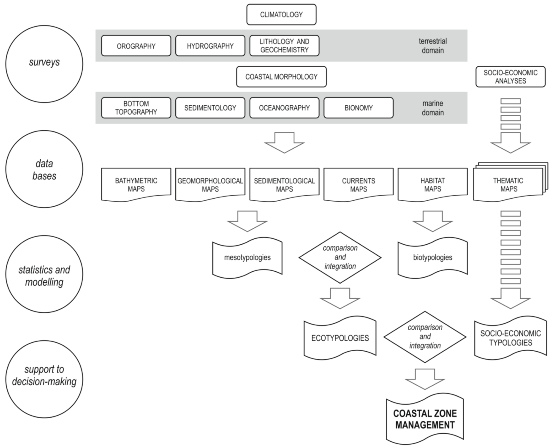
2. Methodological Aspects

2.1. Criteria and Definitions for Diagnostic Cartography

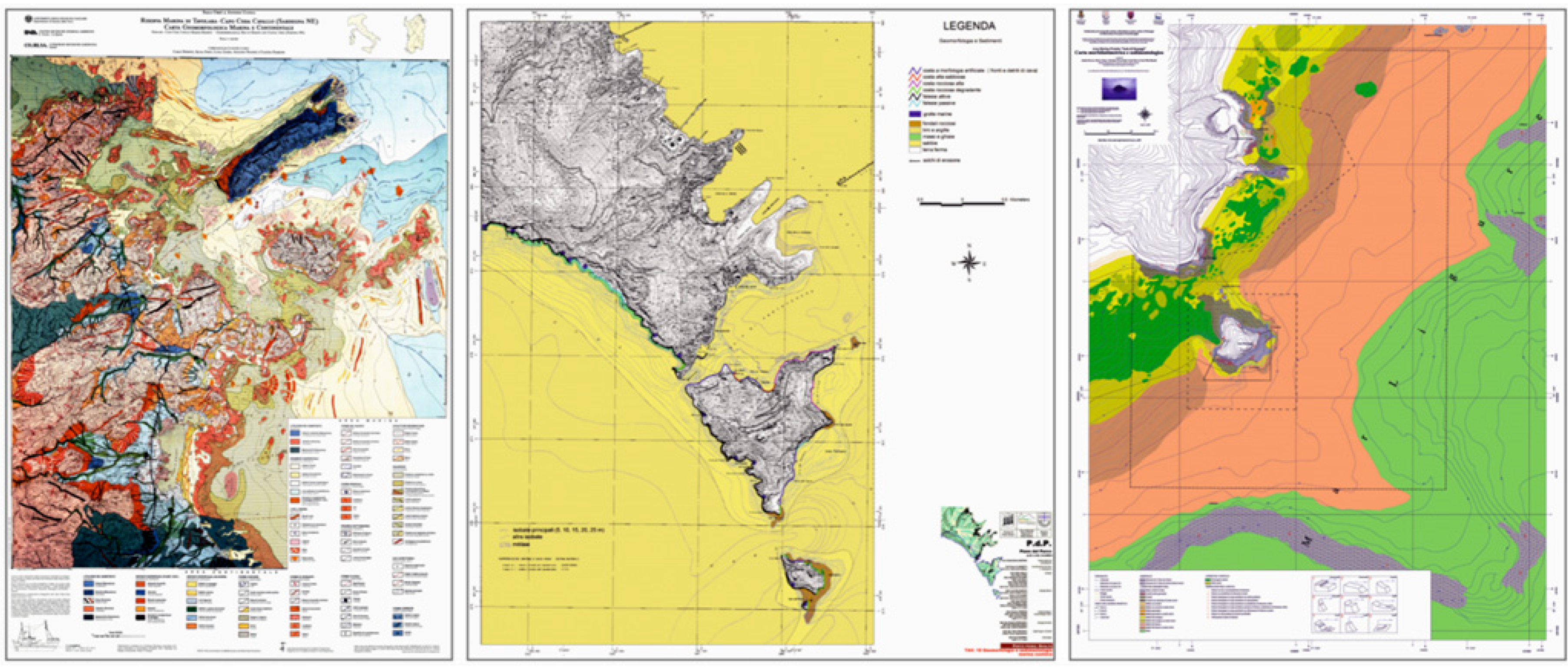
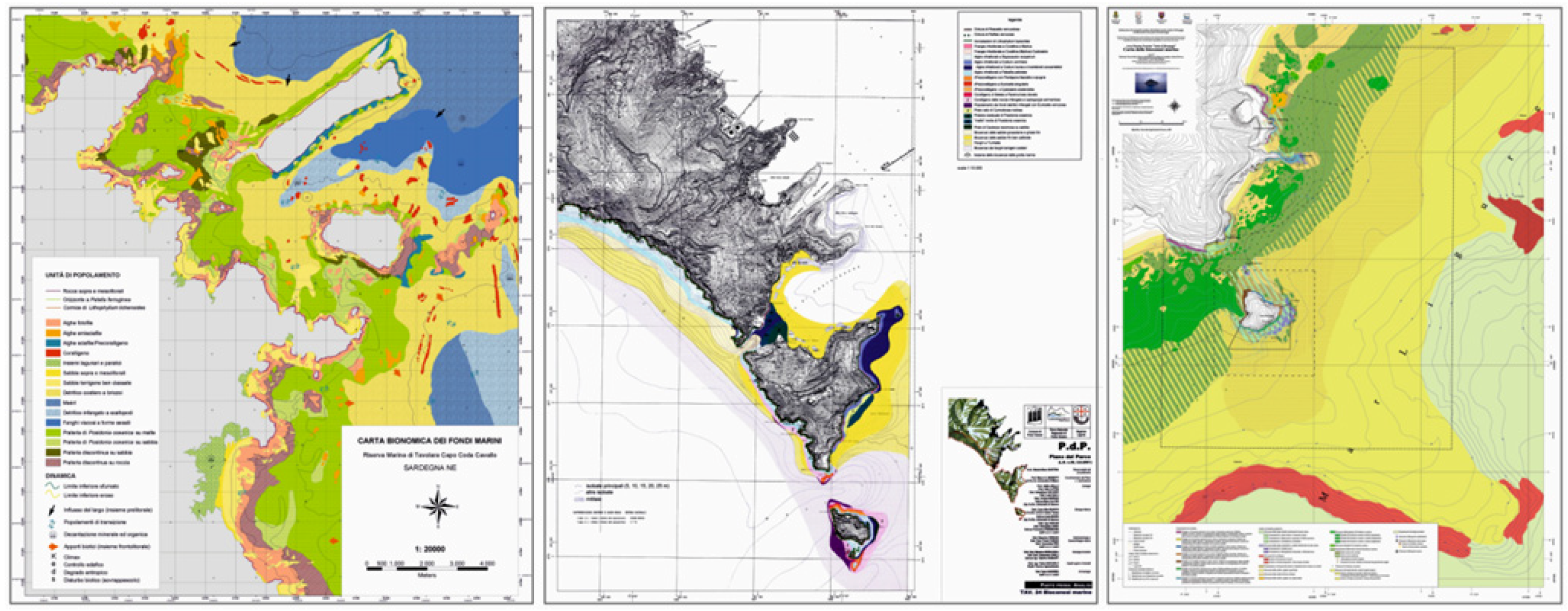
Diagnostic cartography consists in the employment and cartographic representation of a set of synthetic indicators for the evaluation of the territory to be managed [24,46]. The need for diagnostic tools for the coastal zone has been enunciated in 1992 by Agenda 21, which proposed seven program areas including the integrated management and sustainable development of coastal and marine areas [47]. As a result of the agenda, coastal states committed themselves to ICZM under their national jurisdiction.

The concepts of sustainable development and integrated management, as enunciated by the agenda, represented an important political and cultural change in the perspective of the management of the coastal zone. Globally, it was decided to pursue the objective of sustainability, and the way of achieving the goal of integrated management was defined.

Earlier perspectives of marine coastal management characterized a period of multidisciplinary studies aimed at collecting environmental information in core areas, where economic development had to be implemented (for major examples in Italian seas, see [48,49,50,51,52,53]). More recently, procedures have been developed aimed explicitly at creating tools for coastal management [54]. Such procedures are used to evaluate the quality and quantity of the manageable area in a territory. The same approach can be applied to comparing the natural heritage value of different areas within the same territory or of the same area in time, providing tools for territorial planning and for measuring impacts, respectively.

One of the most relevant innovations of Agenda 21, besides the conceptual perspective of management, was the adoption of a well-designed tool for the environmental diagnostics. From a scientific point of view, this corresponded to a shift from an engineering-based management [55] to EBM. Information on environmental components became insufficient, and tools for the evaluation of ecosystems types, status, functioning, and services had to be developed [56].

After the definition of coastal zone management by the Agenda, national and international organisms started to develop a number of legislative instruments, and conservation ecology made a huge effort in the conceptual definition of schemes whose goal is the harmonization of legislation, socioeconomy and environment within efficient socioecosystems [57]. This may be achieved only by the employment of a set of indicators accounting for the legislative constraints, the environmental quality and the sustainable use of resources for the economic development.

From a technical point of view, the mapping of legislative constraints allows for the identification of coastal marine areas where protection is mandatory. Similarly, maps of the environmental quality, of its vulnerability and susceptibility to human use represent the instruments needed by managers to achieve sustainable development.

These are part of the suite of cartographic tools we propose in the present paper, along with study case applications that we developed during recent research in Italian MPAs. Although from a conceptual point of view, ICZM and EBM have reached their maturity, practical application of tools for diagnostic cartography still remain scarce. In all procedures of environmental evaluation, it is customary to merge information on habitats (or, more precisely, biocoenoses, associations, and facies) [58,59] and species, with estimates of their naturalistic and economic interest and their vulnerability and susceptibility [30].

To date, one of the main obstacles to the application of environmental diagnostics procedures in the Mediterranean Sea is represented by the scarce effort spent in the evaluation of habitats properties, thereby impairing the development of environmental indices [60]. Specific biotic indices have recently been developed to evaluate water quality using macrobenthos [61,62,63], seagrass [64,65] or littoral macroalgae [66,67]. A list of indices of interest for environmental diagnostics has been prepared at Mediterranean Sea level, following the criteria first employed in France for the implementation of the EU Habitats Directive in the terrestrial realm [68]. In particular, the Regional Activity Centre for Specially Protected Areas (RAC SPA) of UNEP has elaborated the evaluation scores for 148 Mediterranean marine habitats at different hierarchical levels [69]. These evaluation scores were established through Best Expert Judgement (BEJ) for the following environmental values: (i) vulnerability; (ii) aesthetics; (iii) economics; and (iv) naturalness [70]. The tools, including formulaic arrays, proposed here stem from the combination of the above values for the development of thematic maps and tools aimed at the management of the marine territory.

2.2. Map Production

The procedures of environmental diagnostics embrace two levels: (1) the characterization, based on the analysis of abiotic and biotic characteristics of the environment in order to identify types; (2) the evaluation, based on the analysis of these types to define their status and values. Both levels use cartography as an instrument for management. Here, we propose a suite of cartographic tools for the environmental diagnostics to be applied to the marine realm. Three thematic maps are used for the first level of the environmental diagnostic (characterization), and four for the second (evaluation). The maps for environmental characterization are: (i) morphobathymetry and sedimentology, (ii) habitats; and, (iii) natural emergencies. The maps for environmental evaluation are: (i) environmental degradation and risk; (ii) weighted vulnerability; (iii) environmental quality; and, (iv) susceptibility to human use. These will be described using as study cases three different Italian MPAs employing different cartographic scales: 1:10,000 for the MPA “Arcipelago di Portovenere,” 1:25,000 for the MPA “Tavolara-Punta Coda Cavallo,” and 1:2,000 for the MPA “Isola di Bergeggi.” All maps, at their full size, can be freely downloaded from the SEAMap site [45].

To produce the maps for the diagnostics of the marine territory, a first methodological premise consists in dividing the study areas into territorial units (TUs) [40]. TUs may be zones, chosen according to environmental criteria, but it is more appropriate that TUs correspond to cells of a grid adequately chosen to introduce the numerical information into a Geographical Information System (GIS), where it can be elaborated, processed and interrogated in a versatile manner. The employment of a grid implies, however, the choice of the cell size. This choice is the result of a compromise between the following conditions: (i) TUs represent the information with a sufficient resolution (according to the scale of the map adopted); (ii) TUs are comparable in view of the goal of the evaluation; and, (iii) TUs are easily linked with a relational database into a GIS. Typically, TUs are built as fractions of the UTM (Universal Transverse Mercator) grid with cell sizes varying according to the scale employed. It must be pointed out that the territorial information represented in the cells will remain linked to the nominal scale initially chosen and will dictate the maximum spatial resolution at which information may be retrieved. Enlargements of the map a posteriori are not permitted; as no new information has been introduced, map enlargements will provide only spurious precision, with an illusory impression of greater detail.

Once the TUs have been defined, the second methodological choice to be done is the method for transferring to cells the scores assigned to habitats. There are essentially three ways to do that: (i) the score of a cell is the sum of the scores of all the habitats contained in the cell; (ii) the score of a cell is the mean of all the scores of the habitats contained in the cell; and, (iii) the score of a cell is the maximum of the scores of all the habitats contained in the cell. Each method has advantages and disadvantages (Table 1). Individual habitats’ size (i.e., the area they occupy in the cell) plays a small role in identifying advantages and disadvantages in the score system. The choice depends on the relative weight that it is decided to attribute to the ecodiversity (i.e., the variety of co-occurring habitat) [71] rather than to the absolute importance of the individual habitats. The sum of the scores of individual habitats maximizes the role of ecodiversity on the final score, while the mean and especially the maximum tend to give more weight to the values of individual habitats. In the maps described here, it has been decided to employ the sum of the scores of individual habitats, ecodiversity being considered as an important additional value of the marine territory. However, in order to avoid losing important information on individual habitats showing high scores, additional symbols were used, differing case by case.

Table 1. Criteria to assign a territorial unit with a score on the basis of the scores of the habitats it contains. Advantages and disadvantages of each criterion are indicated.

From Habitat Scores To Territory Scores
1st criterion		cell score is the sum of the scores of all habitats contained in the cell
	advantage	the additional value of ecodiversity in accounted for
	disadvantage	do several low-value habitats equate one high-value habitat?
2nd criterion		cell score is the mean of the scores of all habitats contained in the cell
	advantage	several low-value habitats produce anyway low value-cells
	disadvantage	co-occurrence of low-value and high-value habitats ends in mediocre cells
3rd criterion		cell score corresponds to the maximum score of any single habitat contained in the cell
	advantage	the occurrence of high-value habitats is shown out
	disadvantage	ecodiversity is ignored

Table 1. Criteria to assign a territorial unit with a score on the basis of the scores of the habitats it contains. Advantages and disadvantages of each criterion are indicated.

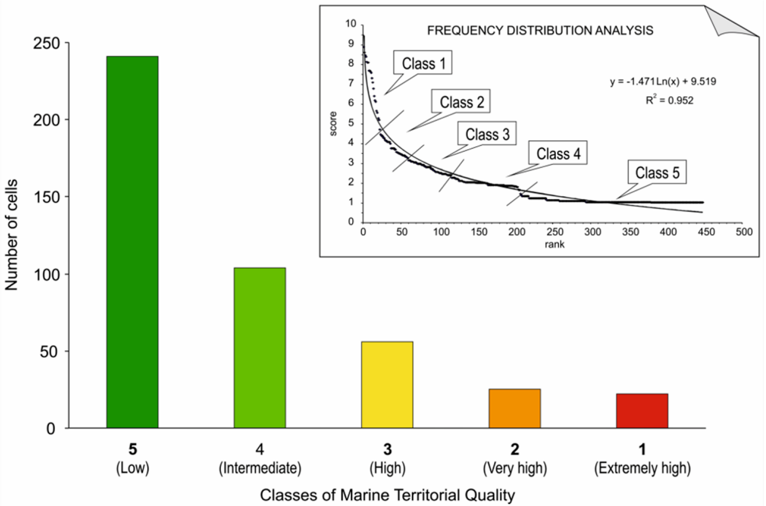
From Habitat Scores To Territory Scores
1st criterion		cell score is the sum of the scores of all habitats contained in the cell
	advantage	the additional value of ecodiversity in accounted for
	disadvantage	do several low-value habitats equate one high-value habitat?
2nd criterion		cell score is the mean of the scores of all habitats contained in the cell
	advantage	several low-value habitats produce anyway low value-cells
	disadvantage	co-occurrence of low-value and high-value habitats ends in mediocre cells
3rd criterion		cell score corresponds to the maximum score of any single habitat contained in the cell
	advantage	the occurrence of high-value habitats is shown out
	disadvantage	ecodiversity is ignored

Finally, the third methodological aspect consists in dividing the final territorial scores of the cells into a reasonable number of classes, to synthesize information. The following procedure was adopted (Figure 1): (i) the scores of all the cells contained in each map were subjected to frequency distribution analysis; (ii) thanks to the analysis, “natural” breaks in the distribution curve were evidenced; (iii) such breaks were equated to the boundaries of five classes of different amplitude (normally increasing from the class expressing the highest scores to the one expressing the lowest scores); (iv) a colour was assigned to each class using red, orange, yellow, light green and dark green, in the order, to indicate decreasing management attention. At first glance, this colour scale may appear contrary to a common usage in the evaluation of the status of water bodies, where the red colour intuitively suggests a bad condition and the green colour a good one. The purpose of the present maps, however, is not to highlight TUs that should be improved or restored, but rather TUs that must be administered sustainably. Our colour choice, therefore, followed the logic of the “traffic light”, where red means stop (do not proceed with any concession), yellow means caution, and green means go easy.

Figure 1. Procedure to assign territorial units (grid cells) with evaluation classes through frequency distribution analysis of the scores of the cells contained in every individual map. Five classes were identified whose boundaries were set in correspondence of major breaks in the distribution curve. The example deals with the quality of the marine territory of the MPA “Isola di Bergeggi”.

Figure 1. Procedure to assign territorial units (grid cells) with evaluation classes through frequency distribution analysis of the scores of the cells contained in every individual map. Five classes were identified whose boundaries were set in correspondence of major breaks in the distribution curve. The example deals with the quality of the marine territory of the MPA “Isola di Bergeggi”.

3. Use and Implications of Territorial Maps

3.1. Maps for Marine Territory Characterization

The morphobathymetric and sedimentological maps (Figure 2) and the habitats maps (Figure 3), should be already familiar to both scientists and managers, and are already part of the usual tools for the management of the marine coastal zone. Although they provide the basis for all the remaining maps, they will not be discussed further in the present paper.

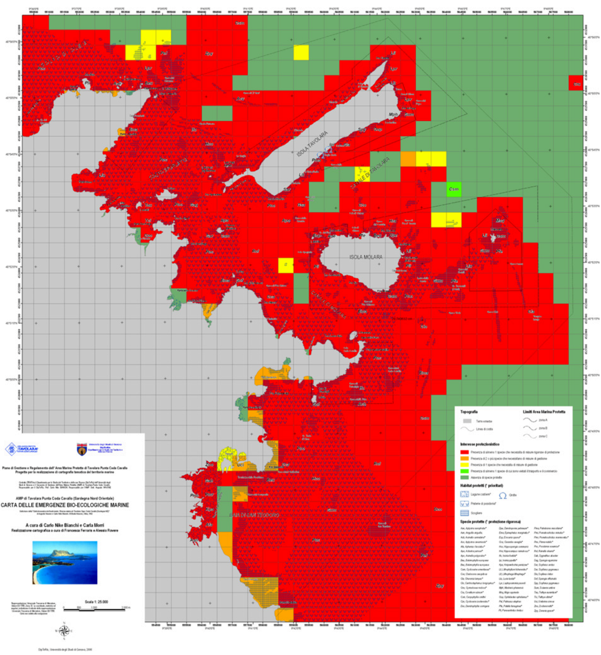
Map of Marine Natural Emergencies

A natural emergency is a natural feature that requires intervention to prevent a worsening of the environment status. In conservation biology, the term “emergencies” is usually referred to species or habitats that, because of their natural value, have to be considered as part of the biological and ecological heritage of a site. More recently, the term has being extended to include marine geological heritage [71,72,73], leading to an integrated view of the marine natural heritage [75,76].

Early experiences of thematic mapping of nature emergencies in the Mediterranean Sea focused on species and habitats that the scientific community defined as in need of protection measures [77,78,79]. Most of these species and habitats are today included in international conventions and UE directives

Figure 2. Reproduction at reduced scale of the morphobathymetric and sedimentological maps of the three MPAs considered. Left to right: “Tavolara-Punta Coda Cavallo” (original scale 1:25,000), “Arcipelago di Portovenere” (original scale 1:10,000), “Isola di Bergeggi” (original scale 1:2,000). These maps, at their full size, can be freely downloaded from the SEAMap site [45].

Figure 2. Reproduction at reduced scale of the morphobathymetric and sedimentological maps of the three MPAs considered. Left to right: “Tavolara-Punta Coda Cavallo” (original scale 1:25,000), “Arcipelago di Portovenere” (original scale 1:10,000), “Isola di Bergeggi” (original scale 1:2,000). These maps, at their full size, can be freely downloaded from the SEAMap site [45].

Figure 3. Reproduction at reduced scale of the marine habitats maps of the three MPAs considered. Left to right: “Tavolara-Punta Coda Cavallo” (original scale 1:25,000), “Arcipelago di Portovenere” (original scale 1:10,000), “Isola di Bergeggi” (original scale 1:2,000). These maps, at their full size, can be freely downloaded from the SEAMap site [45].

Figure 3. Reproduction at reduced scale of the marine habitats maps of the three MPAs considered. Left to right: “Tavolara-Punta Coda Cavallo” (original scale 1:25,000), “Arcipelago di Portovenere” (original scale 1:10,000), “Isola di Bergeggi” (original scale 1:2,000). These maps, at their full size, can be freely downloaded from the SEAMap site [45].

that are being received by national laws. At present, it is therefore possible to introduce a more formal definition of the concept of biological and ecological emergencies to indicate those species and habitats that are explicitly protected by the law. This is a crucial step from the conservation perspective: looking at a map of natural emergencies, a manager can identify the TUs that must be protected, not just habitat and species that should be protected according to naturalists’ opinion.

The EU Habitats Directive is the only listing for habitats, while the remaining norms consider species only. The Habitats Directive focuses mostly on terrestrial habitats, the only marine habitats considered as “priority habitats” being Posidonia oceanica meadows and coastal lagoons. Thus, protected habitats were of limited utility in the development of a territorial index aimed at representing the level of protection required. In addition, P. oceanica is also listed as a protected species, causing redundancy. No specific law protects the geological heritage. As a consequence, the index here utilized was based only on protected species. To this purpose, protected species were divided into three groups.

The first group includes species in need of strict protection, as explicitly stated in the Annex IV of the Habitats Directive. By analogy, the species listed in the Appendices 1 and 2 of the Bern Convention (special protection), in the Annex II of the Habitats Directive (species requiring designation of special areas of conservation) and in the Annex II of the Barcelona Convention (threatened species) are added to this group.

The second group includes the species that require being managed. Such are the species listed in the Annex V of the Habitats Directive (whose taking from the wild can be restricted) or in the Annex III of the Barcelona Convention (whose exploitation is regulated). Similarly, the species listed in the Appendix 3 of the Bern Convention need appropriate and necessary legislative and administrative measures.

Finally, the third group includes those endangered species whose trading is limited but for which no particular conservation measure in the wild is required. These are the species listed in the Annexes of the Washington Convention on the International Trade in Endangered Species of wild fauna and flora (CITES).

To represent visually on the map the level of protection required by law, each cell was ranked according to the occurrence of species belonging to the three groups and then assigned with a specific colour according to the following scale:

• (1) Red: occurrence of at least one species of the first group (strict protection required);
• (2) Orange: occurrence of two or more species of the second group (management required);
• (3) Yellow: occurrence of one species of the second group (management required);
• (4) Light green: occurrence of at least one species of the third group (trade regulated);
• (5) Dark green: no protected species are present.

The synthetic information provided by colours is the most important for management, showing the level of attention that should be given to distinct areas of the marine territory. In addition, the occurrence of a species is indicated on the map by an alphabetic code inspired by the species’ Latin binomial name (normally the first letter of the genus name and the first two letters of the species name), while the occurrence of ecological (protected habitats) and geological emergencies (interesting geothemes) is indicated by special symbols overlaid on the background colour map (Figure 4).

While the distribution of habitats and geothemes may be directly deduced from the habitat map and the morphobathymetric and sedimentological map, respectively, information on the punctual distribution of protected species is rarely available. To date, few MPAs, if any, have realized the complete inventory of the species living within their borders. Evidently, it is not possible to manage species that have not been found [79], and the inventory of the biological emergencies should be a priority among the research activities of the MPAs. To realize the map of natural emergencies, information on protected species occurrence and distribution has been compiled from:

(1) bibliographic data, including “grey literature”; (2) data obtained from divers and fishermen, either amateurs or professional; (3) field data collected in the frame of various research programs [68]. As a result, information on protected species occurrence and distribution utilized for the map of marine natural emergencies has to be considered preliminary, surely incomplete and probably imprecise.

Figure 4. Reproduction at reduced scale of a map of marine natural emergencies. The example illustrates the MPA “Tavolara-Punta Coda Cavallo” (original scale 1:25,000). This and similar maps can be freely downloaded, at their full size, from the SEAMap site [45].

Figure 4. Reproduction at reduced scale of a map of marine natural emergencies. The example illustrates the MPA “Tavolara-Punta Coda Cavallo” (original scale 1:25,000). This and similar maps can be freely downloaded, at their full size, from the SEAMap site [45].

3.2. Maps for Marine Territory Evaluation

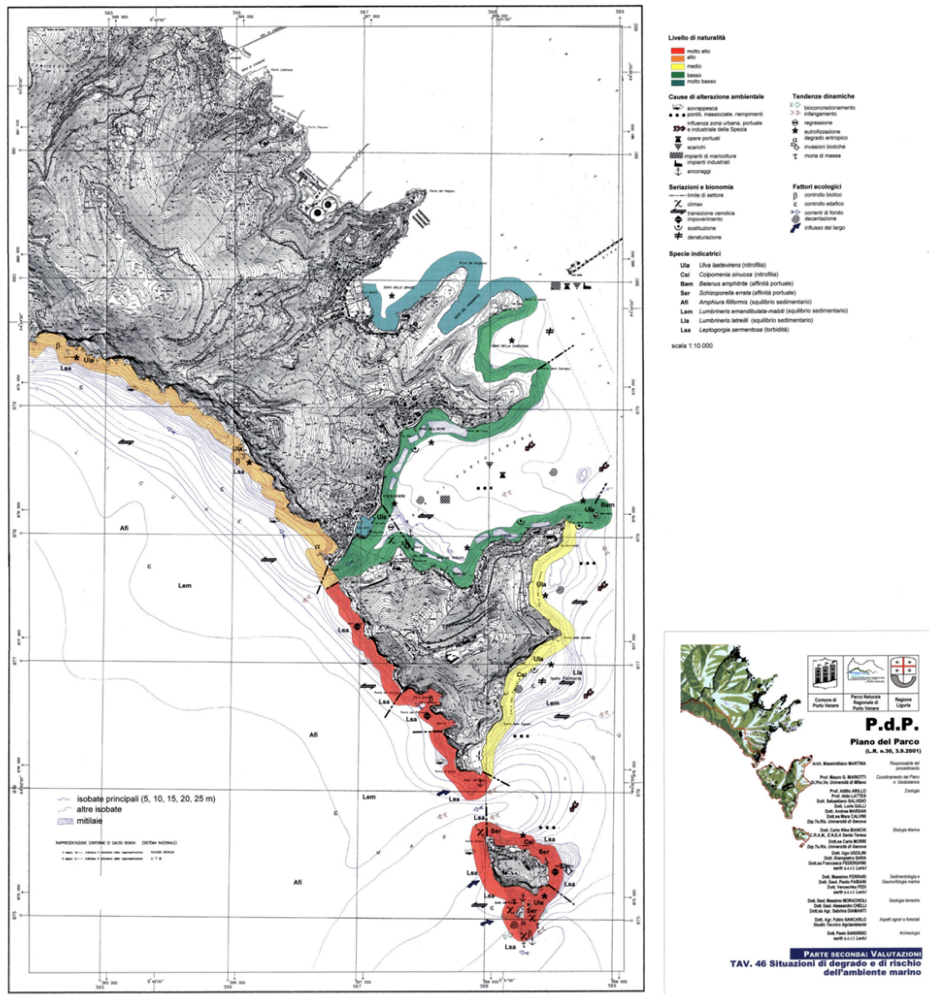
3.2.1. Map of Degradation and Risk

The evaluation of the degradation of the marine territory and the assessment of potential risks to which it is subject, require scuba surveys and optical and acoustic imagery, together with socioeconomic information about the intensity of marine resources exploitation and other human pressures.

Degradation is normally defined as the inverse of the naturalness of the territory [81]: human pressures take the territory away from its “natural” condition, so that the greater the anthropization, the higher the degradation [82]. Although widely accepted by naturalists [83], this definition is questioned on land by landscape architects, who maintain that human intervention may improve the value of a territory, as in the case of certain Mediterranean rural agroecosystems, terraced coltures or woodland cares [84]. In the sea, that can be considered one of the last naturalness reservoirs of the planet, anthropization seems always accompanied with degradation; it is difficult to say that harbours, coastal infrastructures or artificial beaches improve marine ecosystems. However, the case of artificial reefs, built to increase fish abundance and diversity, could be debated.

For the map described here, the degradation of the marine territory has been evaluated (semi) quantitatively using a twofold classification [85] that takes into account both the level (intensity and quality) of coastal anthropization (presence of artefacts and infrastructures, urban and tourist development, fishery, etc.) and indices and indicators of alteration of marine ecosystems [33,62,86]. In an era of sliding baselines [87], setting the appropriate reference conditions may become crucial to quantify departure from naturalness [88,89].

The level of degradation is represented on the map by a chromatic scale comprising of five levels (with decreasing naturalness):

• (1) Red: very low degradation (little sign of human presence, marine ecosystems in excellent conditions);
• (2) Orange: low degradation (scarce human presence, limited fishing activity, marine ecosystems in near natural conditions);
• (3) Yellow: mean degradation (moderate human presence and fishing activity, marine ecosystems only slightly altered);
• (4) Light green: high degradation (high human presence and fishing activity, occurrence of anthropogenic waste and artefacts on the seafloor, marine ecosystems altered);
• (5) Dark green: very high degradation (harbours and/or completely urbanized areas, marine ecosystems deeply altered).

Besides colours to classify cells, the map of degradation and risk of the marine territory contains black symbols to inform on potential risks (Figure 5). These are assessed only qualitatively, individuating and locating on the map (Figure 6) putative causes of environmental alteration, ecological factors (that drive ecosystem structure and functioning), bionomy and ecological processes (that impose spatial variation), and series and trends (that illustrate probable change with time). In addition, the occurrence of indicator species is reported with an alphabetic code inspired by the species’ Latin binomial name (Table 2). The ecological indication provided by the occurrence (or, better, abundance) of those species helps define the ecosystem status and does not necessarily convey a direct meaning for protection. Indication about altered sediment setting might be correlated with certain human activities (e.g., beach renourrishment); indication about eutrophication or pollution may represent an early warming of nutrient increase; indication about sea warming informs on the local consequences of the range expansion of warm water species, which may compete with local species; indication about bioconcretioning highlights the potentiality of formation of biogenic substrate (an important aspect of seafloor integrity according to the European Marine Strategy Framework Directive); etc.

Figure 5. Reproduction at reduced scale of a map of the degradation and risk of the marine territory. The example illustrates the MPA “Arcipelago di Portovenere” (original scale 1:10,000). This and similar maps can be freely downloaded, at their full size, from the SEAMap site [45].

Figure 5. Reproduction at reduced scale of a map of the degradation and risk of the marine territory. The example illustrates the MPA “Arcipelago di Portovenere” (original scale 1:10,000). This and similar maps can be freely downloaded, at their full size, from the SEAMap site [45].

Figure 6. Examples of symbols of degradation and risk of the marine territory. Maps that use these symbols can be freely downloaded, at their full size, from the SEAMap site [45].

Figure 6. Examples of symbols of degradation and risk of the marine territory. Maps that use these symbols can be freely downloaded, at their full size, from the SEAMap site [45].

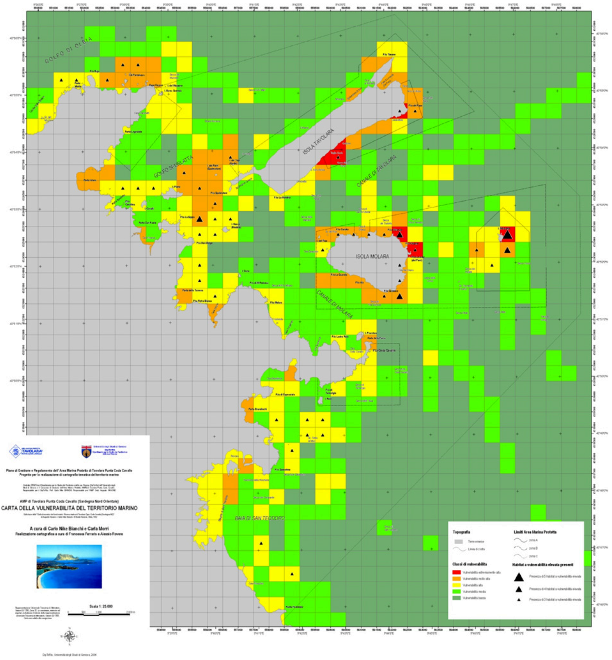
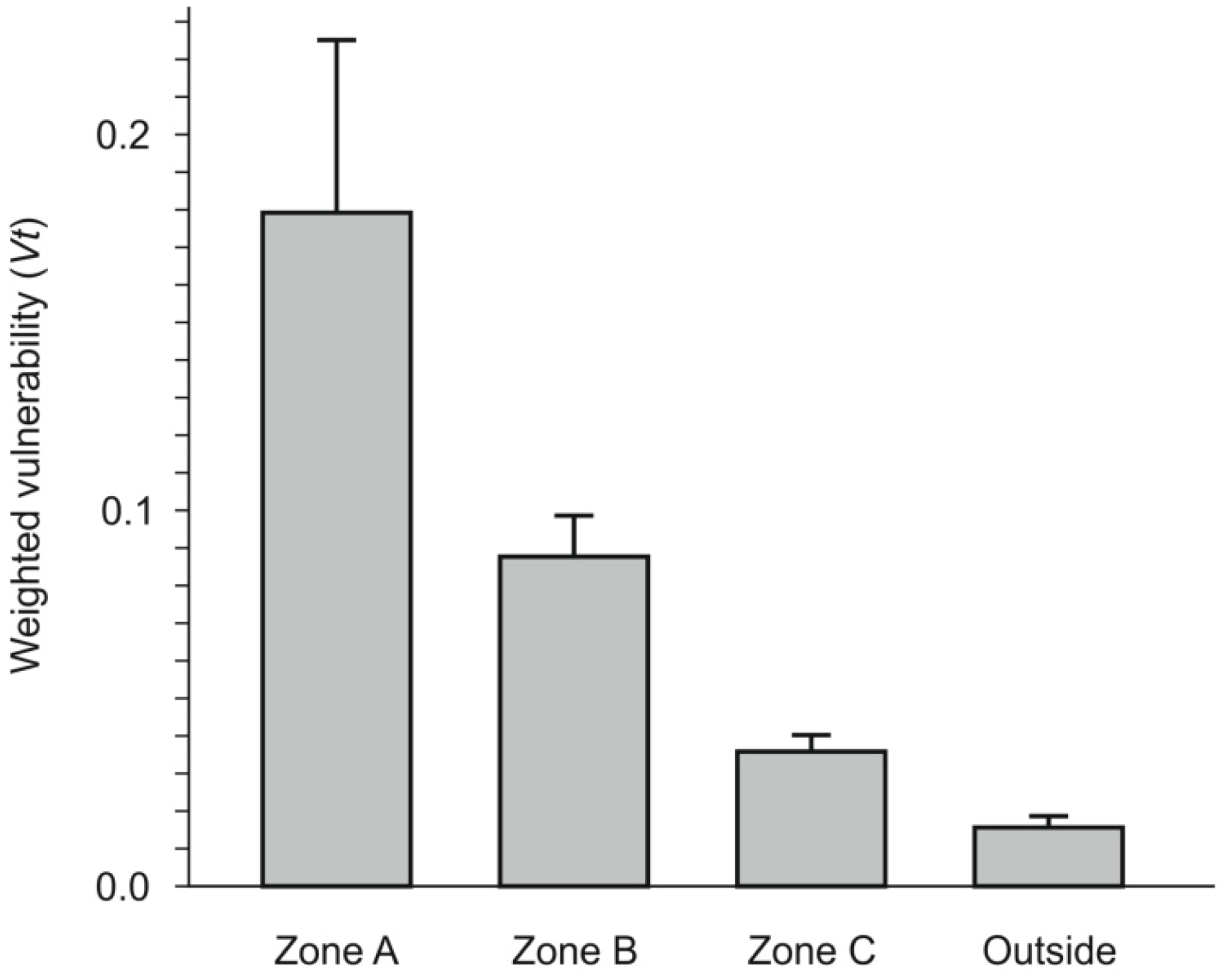
3.2.2. Weighted Vulnerability Map

Vulnerability is defined as the capacity of a habitat to maintain its structure and functions when facing real or potential unfavourable influences. The higher the vulnerability, the greater the probability of alteration following an impact [90]. A vulnerability map provides managers with information on the vulnerability of each TU and on the location of the most fragile ecosystems. Consulting such a map helps to plan specific monitoring activities, to undertake efficient protection measures, and to develop initiatives to mitigate the consequences of unwanted change.

The map of the vulnerability of the marine territory uses the information contained in the habitat map. Habitats identified for the map purposes were assimilated as far as possible to those of the RAC SPA list [69], which assigns individual habitats with three distinct levels of vulnerability: elevated, intermediate, and scarce [70]. Habitats with elevated vulnerability were scored “3”, habitats with intermediate vulnerability were scored “2”, habitats with scarce vulnerability were scored “1.” The vulnerability score of each habitat was then divided by the number of cells where the habitat is present, in order to weight its vulnerability on its frequency in the whole area. This aspect, often neglected in punctual studies, maintains that a rarer habitat is intrinsically more vulnerable than an equally vulnerable but commoner habitat. As an example, imagine that an MPA (or any coastal tract to be managed) harbours thousands of hectares of P. oceanica meadows, but only a small number of

Table 2. List of the indicator species utilized for the map of degradation and risk of the marine territory of the MPA “Isola di Bergeggi,” which can be freely downloaded at full size from the SEAMap site [45]. The code with which the species occurrence is mapped, the Latin name of the species, the higher taxon to which it belongs, and the environmental information provided are reported left to right. Individual species do not necessarily occur in the same TU, thus indicating different environmental conditions in different parts of the area.

Code	Species	Higher taxon	Indication
Aca	Axinella cannabina	Porifera	sea warming
Ama	Aphelochaeta marioni	Annelida	rapid and/or intense settling
Amu	Aspidosiphon muelleri	Sipuncula	organic settling
Apo	Axinella polypoides	Porifera	sea warming
Avi	Arthrocladia villosa	Ochrophyta	bottom currents
Cca	Capitella capitata	Annelida	pollution
Cgi	Corbula gibba	Mollusca	organic and fine particle accumulation
Cno	Cymodocea nodosa	Tracheophyta	ecological substitution
Cra	Caulerpa racemosa	Chlorophyta	biological invasion
Cse	Chaetozone setosa	Annelida	inorganic settling
Csi	Colpomenia sinuosa	Ochrophyta	eutrophication
Csm	Caryophyllia smithii	Cnidaria	slow settling
Dar	Ditrupa arietina	Annelida	sediment instability
Dve	Dasycladus vermicularis	Chlorophyta	sea warming
Eve	Eunicella verrucosa	Cnidaria	turbidity
Evi	Eunice vittata	Annelida	habitat degradation
Gun	Glycera unicornis	Annelida	rapid and/or intense settling
Hmu	Hypnea musciformis	Rhodophyta	sea warming
Lby	Lithophyllum byssoides	Rhodophyta	bioconcretioning
Lin	Lithophyllum incrustans	Rhodophyta	overgrazing
Lla	Lumbrineris latreilli	Annelida	organic and fine particle accumulation
Lsa	Leptogorgia sarmentosa	Cnidaria	turbidity
Lst	Lithophyllum stictaeforme	Rhodophyta	bioconcretioning
Mci	Minuspio cirrifera	Annelida	organic settling
Mga	Mytilus galloprovincialis	Mollusca	eutrophication
Mli	Mesophyllum lichenoides	Rhodophyta	bioconcretioning
Mph	Madracis pharensis	Cnidaria	sea warming
Msp	Myrtea spinifera	Mollusca	organic and fine particle accumulation
Opa	Oculina patagonica	Cnidaria	biological invasion
Pam	Phyllangia americana mouchezii	Cnidaria	sea warming
Pcl	Paramuricea clavata	Cnidaria	benthic-pelagic coupling
Pdi	Pennaria disticha	Cnidaria	sea warming
Pfi	Paradialychone filicaudata	Annelida	habitat degradation
Pfu	Pseudochlorodesmis furcellata	Chlorophyta	sea warming
Ppa	Paralacydonia paradoxa	Annelida	organic and fine particle accumulation
Sco	Syllis cornuta	Annelida	sedimentary instability
Sde	Siphonoecetes dellavallei	Arthropoda	organic settling
Sem	Scoletoma emandibulata mabiti	Annelida	rapid and/or intense settling
Ser	Schizoporella errata	Bryozoa	eutrophication
Spe	Sporochnus pedunculatus	Ochrophyta	bottom currents
Tdi	Tellina distorta	Mollusca	sedimentary instability
Tfl	Thyasira flexuosa	Mollusca	mineral settling
Tfr	Tricleocarpa fragilis	Rhodophyta	warm waters
Tov	Timoclea ovata	Mollusca	habitat degradation
Uin	Ulva intestinalis	Chlorophyta	eutrophication
Ula	Ulva laetevirens	Chlorophyta	eutrophication

Table 2. List of the indicator species utilized for the map of degradation and risk of the marine territory of the MPA “Isola di Bergeggi,” which can be freely downloaded at full size from the SEAMap site [45]. The code with which the species occurrence is mapped, the Latin name of the species, the higher taxon to which it belongs, and the environmental information provided are reported left to right. Individual species do not necessarily occur in the same TU, thus indicating different environmental conditions in different parts of the area.

Code	Species	Higher taxon	Indication
Aca	Axinella cannabina	Porifera	sea warming
Ama	Aphelochaeta marioni	Annelida	rapid and/or intense settling
Amu	Aspidosiphon muelleri	Sipuncula	organic settling
Apo	Axinella polypoides	Porifera	sea warming
Avi	Arthrocladia villosa	Ochrophyta	bottom currents
Cca	Capitella capitata	Annelida	pollution
Cgi	Corbula gibba	Mollusca	organic and fine particle accumulation
Cno	Cymodocea nodosa	Tracheophyta	ecological substitution
Cra	Caulerpa racemosa	Chlorophyta	biological invasion
Cse	Chaetozone setosa	Annelida	inorganic settling
Csi	Colpomenia sinuosa	Ochrophyta	eutrophication
Csm	Caryophyllia smithii	Cnidaria	slow settling
Dar	Ditrupa arietina	Annelida	sediment instability
Dve	Dasycladus vermicularis	Chlorophyta	sea warming
Eve	Eunicella verrucosa	Cnidaria	turbidity
Evi	Eunice vittata	Annelida	habitat degradation
Gun	Glycera unicornis	Annelida	rapid and/or intense settling
Hmu	Hypnea musciformis	Rhodophyta	sea warming
Lby	Lithophyllum byssoides	Rhodophyta	bioconcretioning
Lin	Lithophyllum incrustans	Rhodophyta	overgrazing
Lla	Lumbrineris latreilli	Annelida	organic and fine particle accumulation
Lsa	Leptogorgia sarmentosa	Cnidaria	turbidity
Lst	Lithophyllum stictaeforme	Rhodophyta	bioconcretioning
Mci	Minuspio cirrifera	Annelida	organic settling
Mga	Mytilus galloprovincialis	Mollusca	eutrophication
Mli	Mesophyllum lichenoides	Rhodophyta	bioconcretioning
Mph	Madracis pharensis	Cnidaria	sea warming
Msp	Myrtea spinifera	Mollusca	organic and fine particle accumulation
Opa	Oculina patagonica	Cnidaria	biological invasion
Pam	Phyllangia americana mouchezii	Cnidaria	sea warming
Pcl	Paramuricea clavata	Cnidaria	benthic-pelagic coupling
Pdi	Pennaria disticha	Cnidaria	sea warming
Pfi	Paradialychone filicaudata	Annelida	habitat degradation
Pfu	Pseudochlorodesmis furcellata	Chlorophyta	sea warming
Ppa	Paralacydonia paradoxa	Annelida	organic and fine particle accumulation
Sco	Syllis cornuta	Annelida	sedimentary instability
Sde	Siphonoecetes dellavallei	Arthropoda	organic settling
Sem	Scoletoma emandibulata mabiti	Annelida	rapid and/or intense settling
Ser	Schizoporella errata	Bryozoa	eutrophication
Spe	Sporochnus pedunculatus	Ochrophyta	bottom currents
Tdi	Tellina distorta	Mollusca	sedimentary instability
Tfl	Thyasira flexuosa	Mollusca	mineral settling
Tfr	Tricleocarpa fragilis	Rhodophyta	warm waters
Tov	Timoclea ovata	Mollusca	habitat degradation
Uin	Ulva intestinalis	Chlorophyta	eutrophication
Ula	Ulva laetevirens	Chlorophyta	eutrophication

submarine caves, and that both habitats are highly vulnerable according to RAC SPA. To the manager’s eye, however, the local alteration of a small portion of the meadow, although serious, may seem proportionally less important than the alteration of one of the few caves. Weighted vulnerability, therefore, provides managers and administrators with a more useful concept than the rigid idea of “strict protection’” evidenced by the map of marine natural emergencies.

In order to switch from the (weighted) vulnerability of a single habitat to that of a TU, the scores of vulnerability of the habitats in each cell were summed up according to the formula:

Vt_j = Σ_i^m (Vh_i×S_i⁻¹)

(1)

where Vt_j is the weighted vulnerability of the territorial unit j, m is the number of habitats in the cell j, Vh_i is the vulnerability of the habitat i, S_i is the number of cells where the habitat j is present and Vh_i ×S_i⁻¹ is the weighted vulnerability of the habitat i.

Cells are then divided into five classes ordered by decreasing weighted vulnerability, and the corresponding cells are represented on the map with different colours:

• (1) Red: extremely high vulnerability;
• (2) Orange: very high vulnerability;
• (3) Yellow: high vulnerability;
• (4) Light green: mean vulnerability;
• (5) Dark green: low vulnerability.

To complete the information contained in the map, the number of habitats with high vulnerability inside each cell is provided, superimposing black triangles of increasing size to the background colour of the cell (Figure 7). Such a number can be considered as an index of ecological fragility of the marine territory, as it visualizes where the most vulnerable habitats are concentrated independently from the level of territorial vulnerability.

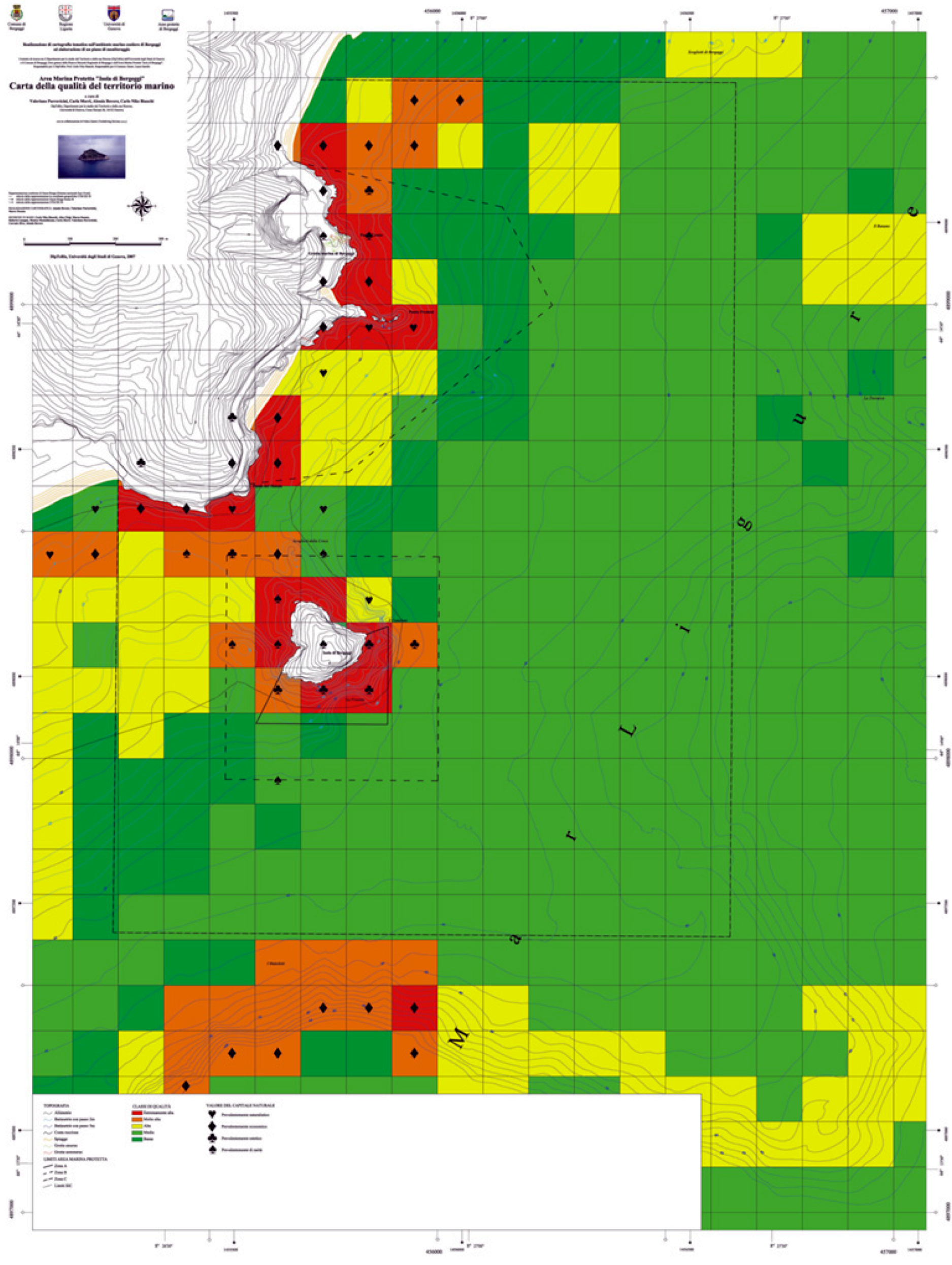
3.2.3. Environmental Quality Map

Assessing marine ecological quality is a major goal for ICZM. Biotic indices were developed in the last decade [91,92] to meet the requests of the EU Water Framework Directive (WFD). However, the ecological quality of the water body does not always correlate with environmental quality as a whole [93]. More recently, the EU Marine Strategy Framework Directive (MSFD) introduced the concept of “seafloor integrity” to improve the assessment of ecological quality [94,95,96,97].

For the purpose of the maps discussed here, a distinction has been made between the potential quality of the marine territory and its (actual) environmental quality. The former is expressed by the value of natural capital “contained” in the territory: the greater the value of the natural capital, the higher the potential quality. The latter combines the former with seafloor integrity, expressed by the status of conservation of the marine territory. It is intuitive that degraded ecosystems lose part of their theoretic value.

The level of degradation is derived from the map of degradation and risk, while the potential quality use the four values identified for habitats by Bardat et al. [68]: (1) the naturalistic value expresses the importance of the habitat for the national or regional natural heritage, due for instance to the presence of endemic species or of unique geomorphologic and ecological features; (2) the economic value

Figure 7. Reproduction at reduced scale of a map of the weighted vulnerability of the marine territory. The example illustrates the MPA “Tavolara–Punta Coda Cavallo” (original scale 1:25,000). This and similar maps can be freely downloaded, at their full size, from the SEAMap site [45].

Figure 7. Reproduction at reduced scale of a map of the weighted vulnerability of the marine territory. The example illustrates the MPA “Tavolara–Punta Coda Cavallo” (original scale 1:25,000). This and similar maps can be freely downloaded, at their full size, from the SEAMap site [45].

reflects the significance of the habitat as a source of monetary income, either through direct exploitation (fishery, tourism, etc.) or indirectly because of the ecosystem services it offers; (3) the aesthetic value is a measure of the relevance of the habitat within the landscape; (4) the rarity value is depending on the frequency of the habitat globally.

Computing the potential quality of the marine territory uses the information contained in the habitat map. Habitats identified for the map purposes were assimilated as far as possible to those of the RAC SPA list [69] in order to assign them with the proposed natural, economic, aesthetic and rarity scores [70]. Each score is arranged from 1 (lowest value) to 3 (highest values), and the four scores for each habitat are then integrated into a synthetic index using the following formula:

Qh_i = (N_i×E_i × A_i × R_i) × k⁽¹⁻ⁿ⁾

(2)

where Qh_i is the synthetic index of quality for the habitat i; N_i, E_i, A_i, and R_i are the scores of naturalistic, economic, aesthetic and rarity values of the habitat i, respectively; k is the maximum value possible (3 in this case) and n is the number of values adopted (4 in this case).

To pass from habitat quality to environmental quality, and taking into account also the status of conservation of the marine territory, the following formula was applied:

Qt_j = [Σ_i^m (Qh_i )] × D_j⁻¹

(3)

where Qt_j is the environmental quality of the cell j, m is the number of habitats in the cell j, Qh_i is the synthetic index of quality of the habitat i, and Dj is the score of degradation of the cell j.

Cells were divided into five classes ordered by decreasing quality and mapped with different colours:

• (1) Red: extremely high environmental quality;
• (2) Orange: very high environmental quality;
• (3) Yellow: high environmental quality;
• (4) Light green: mean environmental quality;
• (5) Dark green: low environmental quality.

The map user is then informed about the prevailing value of the natural capital contained in each cell, superimposing symbols on the background colour: ♥ = naturalistic value; ♦ = economic value; ♣ = aesthetic value; ♠ = rarity value (Figure 8).

The environmental quality is a synthetic measure of the value of the marine territory, useful in all situations that require comparing the natural capital with the human and financial capitals. The indication of the prevailing values provides further detail with management importance, as it suggests the most adequate use of the marine territory. While in the case of an MPA conservation will always be the absolute priority, activities of education and training would ideally take place in TUs with naturalistic value prevailing; sustainable use of natural resources (traditional artisanal fishery) in TUs with economic value prevailing; sustainable ecotourism (including diving) in TUs with aesthetic value prevailing; scientific research in TUs with rarity value prevailing.

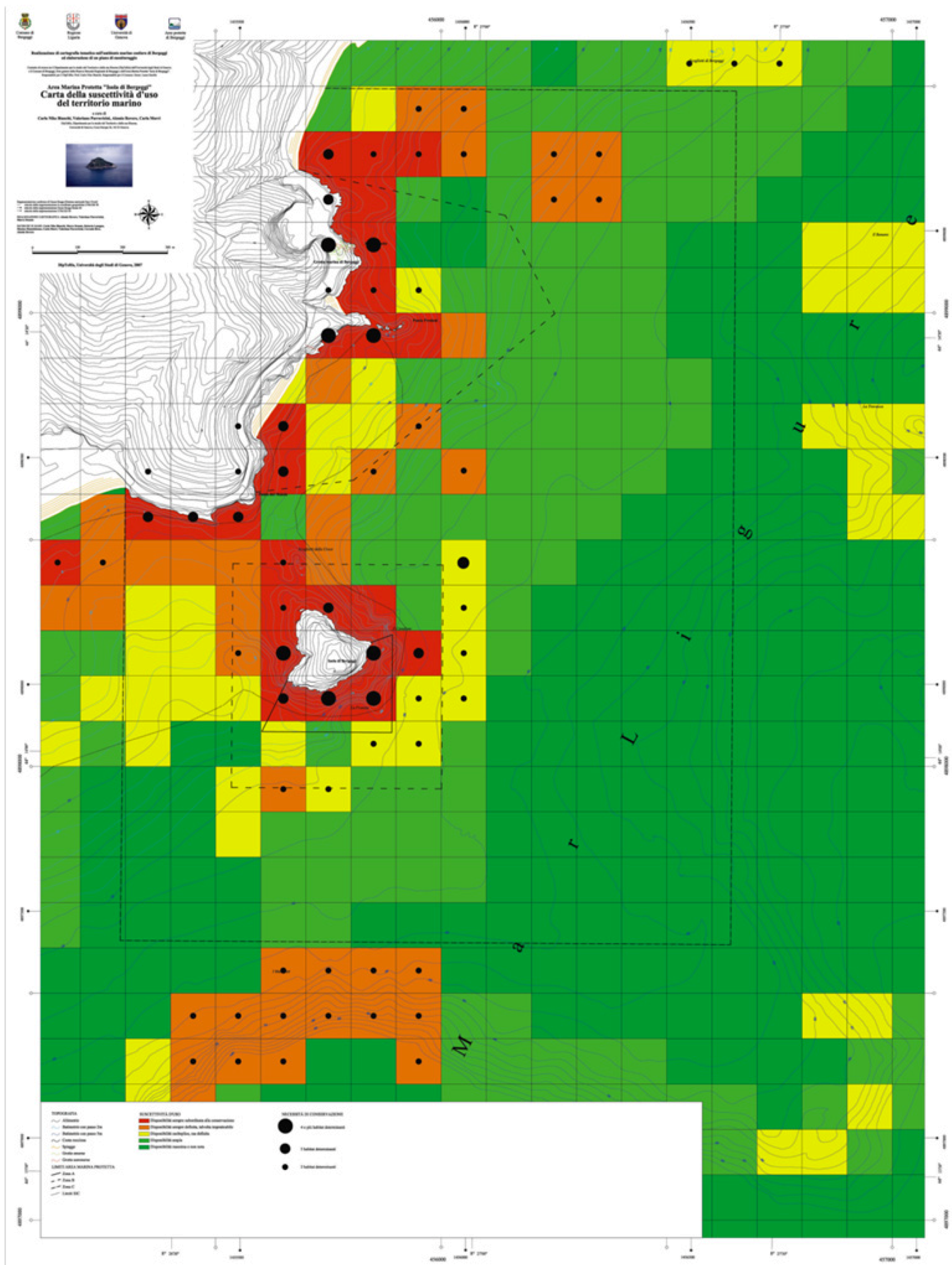
3.2.4. Map of Susceptibility to Use

The map of susceptibility to use is perhaps the most important, as it directly provides managers with indications on the possibility to use a given site for human activities. It is a primary tool for territorial planning and for individuating conflicts or compatibility between conservation and development. While the maps of natural emergencies, of degradation and risk, of weighted vulnerability and of environmental quality are useful to modulate the management strategies when confronting specific needs, the map of susceptibility to use provides a synthesis where to frame decisional choices for

Figure 8. Reproduction at reduced scale of a map of the marine territory quality. The example illustrates the MPA “Isola di Bergeggi” (original scale 1:2,000). This and similar maps can be freely downloaded, at their full size, from the SEAMap site [45].

Figure 8. Reproduction at reduced scale of a map of the marine territory quality. The example illustrates the MPA “Isola di Bergeggi” (original scale 1:2,000). This and similar maps can be freely downloaded, at their full size, from the SEAMap site [45].

management. Although vulnerability and susceptibility are partly overlapping concepts, the former mainly expresses the fact that the habitats in a given TU are fragile and therefore open to damage (not necessarily by human pressures), the latter highlights habitats and species being easily affected by human use, thus directly evocating the idea of sustainability.

The map of (weighted) vulnerability considers only habitats; the map of susceptibility to use merges the information on the occurrence of protected species together with that of important habitats.

As regards protected species, the map of susceptibility to use considers their total number within each cell, in contrast with the map of natural emergencies that highlights the imposed level of protection rather than the total number. Following the logics of emergencies, a strictly protected species is more important than several species that just require some management measures; in terms of susceptibility to use, however, the occurrence of a number of protected species decreases the availability of a site.

As regards habitat importance, the map of susceptibility to use adopts the RAC SPA classification, which individuates three levels: (i) determinant habitats, whose conservation is mandatory; (ii) remarkable habitats, which deserve specific management attention limiting their use; (iii) unimportant habitats, deprived of any particular value and freely available for a sustainable use [70]. Habitats identified for the map purposes were assimilated as far as possible to those of the RAC SPA list [69]; then, a score of 3 has been assigned to determinant habitats, 2 to remarkable habitats, 1 to unimportant habitats.

The total importance of each TU is computed by summing up the importance scores of each individual habitat. Following a linear regression between the total habitat importance and the number of protected species in each cell, an index of susceptibility to use was computed according to the following formula:

St_j = {[Σ_i^m (Ih_i)]² + Eb_j²}^−½

(4)

where St_j is the index of susceptibility to use for the cell j; m is the number of habitats in the cell j, Ih_i is the importance (scored 1 to 3) of the habitat I; Eb_j is the number of protected species in the cell j.

The map of susceptibility to use also contains information about the number of determinant habitats inside each cell, to help evaluating conservation needs (Figure 9): cells with 3, 4, or 5 determinant habitats are marked with black circles of increasing size. The map of susceptibility to use provides a more effective and ductile tool than the mere concept of “strict protection” highlighted by the map of marine natural emergencies.

Cells were then divided into five classes ordered by decreasing susceptibility to use, and coloured differently:

• (1) Red: availability always subordinated to conservation;
• (2) Orange: availability limited and always defined, sometimes impracticable;
• (3) Yellow: availability manifold but defined;
• (4) Light green: broad availability;
• (5) Dark green: maximum availability.

Figure 9. Reproduction at reduced scale of a map of the susceptibility to use of the marine territory. The example illustrates the MPA “Isola di Bergeggi” (original scale 1:2,000). This and similar maps can be freely downloaded, at their full size, from the SEAMap site [45].

Figure 9. Reproduction at reduced scale of a map of the susceptibility to use of the marine territory. The example illustrates the MPA “Isola di Bergeggi” (original scale 1:2,000). This and similar maps can be freely downloaded, at their full size, from the SEAMap site [45].

4. Final Remarks

The experience of the territorial cartographies realized at different scales in three Italian MPAs (Arcipelago di Portovenere, Tavolara-Punta Coda Cavallo, Isola di Bergeggi) provided the opportunity to ponder upon six main issues of general interest: (1) efficacy of the RAC SPA approach; (2) significance of scale for territorial maps; (3) importance of diachronic cartography; (4) adoption of territorial cartography in MPA management; (5) landscape ecology and the rediscovery of bionomic knowledge; (6) MPAs as field laboratories for ICZM. These points should not be taken as the conclusions of the map production work, but rather as free thoughts on the implications of the implementation and use of such maps.

4.1. Efficacy of the RAC-SPA Approach

Adopting the scores proposed by RAC SPA for marine habitats [70] showed the easiest and most practical way to elaborate indices for the environmental evaluation of the marine territory. The availability of a detailed list of habitats (biocoenoses, associations and facies) [58,59], together with their scores of environmental value, is a useful, flexible and standardised tool for all those―either managers or scientists―that have to work on marine territories of the Mediterranean Sea. The habitats defined by RAC SPA [69], have been later introduced into the European Nature Information System (EuNIS) [98]. Of course, integrations and revisions of the RAC SPA list might be necessary, and further research on the marine habitats of the Mediterranean Sea will be needed to keep that list updated.

4.2. Significance of Scale for Territorial Maps

Having produced similar marine territorial maps at three different spatial scales (1:25,000 for Tavolara-Punta Coda Cavallo, 1:10,000 for Arcipelago di Portovenere, 1:2,000 for Isola di Bergeggi) called attention to some conceptual and operative aspects linked to the final scale at which information is represented on maps. Working on GIS platforms might lead to the (wrong) belief that the information in the map is independent by the scale: if representations are vectorial, they can easily be enlarged or reduced without losing image readability. In reality, the information contained in the map depends and will always depend on the scale at which data have been initially acquired. If interpolation and adjustments are acceptable at small scale, they cannot be tolerated at scales larger than that of acquisition.

Ecologists are well aware that the choice of scale does not imply only greater or smaller detail: it also influences the meaning of the phenomena mapped [33]. From the management point of view, ignoring such a reality can lead to huge errors in the evaluation: in the RAC SPA classification, there are cases where a given biocoenosis is considered as unimportant, whilst one (or more) of its associations or facies is determinant [70]. As a consequence, adopting a large scale, which allows for mapping individual association and facies, will classify a given TU as in need of priority conservation effort; on the contrary, choosing a small scale, where only the biocoenosis as a whole is mapped, the same TU will be given a low environmental value. The resulting management choice will be completely different.

It must be clear that the use of a map for ICZM will depend on its scale [99]. The detailed information provided by large scale cartographies (as for instance the maps at 1:2,000 of the MPA Isola di Bergeggi) is already sufficient to take decisions about specific interventions on the territory; the synoptic view offered by small scale cartographies (as for instance the maps at 1:25,000 of the MPA Tavolara-Capo Coda Cavallo) is useful to identify problematic sites where to plan studies of detail. Maps allowing for a synoptic view of a large territory are also indispensable for MPAs whose small extent would apparently ask for large scale maps only: the maps of the MPA Isola di Bergeggi, for instance, will hardly help evaluating the problems that the increasing traffic of the port of Vado Ligure might cause to the marine territory included in the MPA, located only few kilometres downstream [100]. Geospatial models encompassing the major pressures beyond the MPA boundaries represent an important tool for efficient management in the face of complex interactions and high uncertainty [42].

4.3. Importance of Diachronic Cartography

Establishment of MPAs is normally preceded by surveys ending in some sort of cartographic representation of the marine environment (usually the habitat map). This has sometimes caused those who were later charged of managing the MPA, to think that the marine territory was already known and that repeating mapping in time was not necessary [101]. This way of thinking, unfortunately more common than expected among MPA administrators, apparently comes from the belief that marine communities are fundamentally stable and that most observed changes are due to human impacts [102]. It is a conviction, probably rooted in the Linnaean paradigm of balance of nature, which may originate the falsely reassuring tranquillity that, where human impacts are excluded, it is no necessary to invest money to update territorial cartography, monitoring (not always done, however) [11] being enough. Only recently awareness has been growing that marine ecosystem do not tend to, nor fluctuate around, equilibrium: simply, they change, and do so even faster than expected [103,104]. This awareness makes necessary to regularly update territorial mapping and environmental diagnostics also within MPAs.

Time-framed comparisons between cartographies can be performed through diachronic analysis, a procedure commonly adopted in many environmental science applications using GIS [105]. Diachronic cartography includes concordance and discordance maps to represent the surfaces “gained” (positive discordance), “lost” (negative discordance) and unaltered (concordance) between two distinct periods [106]. Historical cartographies of the marine territory, when available, represent a precious heritage for management. However, ancient maps may not be completely reliable due to the different techniques employed [106,107].

With which periodicity should mapping of the marine territory be repeated? Perhaps there is no single answer, much depending on the local biogeographic, ecologic, and anthropogenic peculiarities. Recent experiences of diachronic cartography in Italy illustrated unexpected change in marine coastal habitats during the last two decades [105,106,107,108,109], often due to increased human pressures along the coastline [110]: repeating cartography at least every 10 years should therefore be desirable.

4.4. Adoption of Territorial Cartography in MPA Management

One of the main goals of the procedures for environmental assessment is obtaining a ranked classification of the different portions of the marine territory needing protection, functional to draw an objective zoning of the area under consideration [111,112]. However, the resulting cartography is extremely useful not only to start the management plan in the initial phase but also when a MPA has been fully established and the protection regime enforced, and diachronic cartography allows verifying the results of the protection measures on the territory. To date, the only tool adopted to evaluate the efficiency of protection is monitoring fish stocks [113]. Fish generally show the best descriptors of the so-called “reserve effect” and have a major impact on public opinion and administrators [114]. Attempts at evaluating reserve effect through the analysis of the status of protected habitats and species other than fish are less frequent.

Zoning of most MPAs envisages three zones with different protection levels: zone A (full protection), zone B (partial protection) and zone C (general protection) [115]. All the territorial maps here described showed consistent with the zoning imposed on the MPAs studied: both vulnerability and quality of the marine territory decreased moving from zone A, to zone B, to zone C and, finally, to areas outside the AMP boundaries (Figure 10); on the contrary, susceptibility to use increased moving from zone A, to zone B, to zone C and, finally, to the areas outside the AMP boundaries. It must be underlined that all these indices are based only on the occurrence of habitats and species, and do not take into account the level of protection. Evaluation scores and protection levels are statistically independent and their congruence should be considered as an evidence of a right choice for zoning. Otherwise, it might be opportune reconsidering the current zoning.

4.5. Landscape Ecology and the Rediscovery of Bionomic Knowledge

Although familiar to everybody, “landscape” as a concept has not yet a unique and rigorous definition. From a scientific point of view, the term landscape was born in geography to define the hierarchical assembly of the characters of a region, across all the realms of nature [116]. Each specialist, however, emphasizes the aspects of his/her discipline. To the geologist, landscape is the shape of the relief, to the botanist the typology of the vegetal cover, to the architect the footprint of the human culture, to the ecologist the relationships between ecological processes and spatial organization. Landscape ecology considers that ecosystem functioning depends on environmental heterogeneity, and sees as salient points of landscape studies the complexity of the environmental mosaic and its spatial organisation, hierarchies, structures, processes and changes [117]. The space where organisms and environment interact is never homogeneous, but diversifies along gradients of various factors; it is environmental heterogeneity that defines a landscape. Landscape ecology questions the role that environmental heterogeneity plays in originating or modifying ecological processes. Its first aim is to describe this heterogeneity, characterizing the habitats that occur in a given area and quantifying their distribution. It is therefore obvious that cartography is a valuable tool for the analysis of the landscape and that the principles of landscape ecology are fundamental for territorial diagnostics.

Last but not least, a complete and updated territorial cartography is an essential tool for routine management actions, from the release of concessions to the assessment of impacts.

Independently from the specific definition that the term landscape may assume, it always carries an idea of aesthetic and emotional perception by humans. Thus, there is no landscape without perception. Landscape ecology originated on land, where the visual perception of the environment is common experience. On the contrary, most humans, including scientists and administrators alike, do not have a perception of the marine environment, often seen as just a large expanse of salt water. Humans are aliens in the sea, and only in the last decades modern video and diving techniques have allowed people to appreciate the underwater seascape, with its astonishing beauty and fragility [118]. The idea that the ecological problems in the sea are similar to those known on land for a longer time, is therefore a recent acquisition [39].

Figure 10. The relation between the value of the marine territory and the zoning imposed onto the MPA. The example refers to the weighted vulnerability of the MPA “Tavolara-Punta Coda Cavallo.”

Figure 10. The relation between the value of the marine territory and the zoning imposed onto the MPA. The example refers to the weighted vulnerability of the MPA “Tavolara-Punta Coda Cavallo.”

On land, the cognitive tools for managing landscape originate from the knowledge gained with phytosociology; in the sea, similar tools are offered by bionomy, for which the Mediterranean school has always been in the van [119]. Bionomy (or bionomics) is a term only vaguely familiar to native English-speaking scientists. In most English dictionaries, it is synonymous with ecology. In reality, bionomy (from the Greek bios and nomos, the latter in turn from nemò = I distribute) refers specifically to the part of ecology that studies the distribution of organisms and their assemblages along ecological gradients to identify zones and to understand the link between habitats and species [120]. It is therefore of prime importance that basic research in marine ecology does not lose the bionomic wisdom linked with habitat knowledge and the use of indicator species for territorial diagnostics, for which there is a long Mediterranean tradition [121,122,123,124,125]. Adoption of biological and ecological indicators for environmental assessment is also recommended by international organizations such as UNEP and UNESCO [126,127].

4.6. MPAs as Field Laboratories for ICZM

The marine territorial maps described in this paper represent the first concrete attempt in Italy to test an approach proposed more than 20 years ago [46]. Merging abiotic (“mesotypologies”) and biotic (“biotypologies”) classifications of the natural environment allows producing “ecotypologies” [24] that can be in turn combined with economic and social typologies on a common cartographic base in view of ICZM (Figure 11). Integrating ecology and socioeconomy has become common practice for both environmental protection [128,129] and restoration [130] and stands at the base of marine spatial planning (MSP) [42]. MSP is a process that informs on the spatial distribution of activities in the sea, so that existing and emerging uses can be maintained, use conflicts reduced, and ecosystem health and services protected and sustained for future generations [131].

Figure 11. Scheme of the procedure for coupling ecological and socioeconomical typologies as a guide to ICZM (modified from Bianchi and Zattera [46]).

Figure 11. Scheme of the procedure for coupling ecological and socioeconomical typologies as a guide to ICZM (modified from Bianchi and Zattera [46]).

To date, three MPAs (Arcipelago di Portovenere, Tavolara-Punta Coda Cavallo, Isola di Bergeggi) are the first and only Italian administrations that have a complete marine territorial cartography, not just the habitat map (when existing!). MPAs represent a precautionary and ecosystem-based approach to the management of the sea [132], but MPAs alone are not sufficient to successfully support healthy coastal ecosystems and sustain human uses of the sea [131]. It may sound paradoxical that only MPAs, which are already devoted primarily to conservation, have tools that in theory would be more useful to other coastal territorial organizations that have to cope with growing urban, industrial and harbour uses. Habitats and species in need of legal protection occur all along the coastline, not only within MPAs. It is a difficult task, for administrators, to conciliate socioeconomic development and marine biodiversity protection. In most conservation laws, there is no clear definition of what must be meant by “protection,” as prohibitions are seldom explicit: harvesting and killing of protected species are obviously unacceptable, but what about habitat alteration? and what kind of alteration? to what degree? Environmental alterations due to human impacts can hardly be discriminated from those due to climate change [133]. MPAs may represent the reference condition to tell natural and human influences apart [101]. MPAs may act as field laboratories for developing and testing guidelines for ICSM and assisting territorial administrators in deciding what can be done and what should be avoided where no defined legal restriction is operating. ICZM needs beneficiating from conceptual wealth and creativity: maps such as those described in the present paper represent a useful and precious tool.

References

1. Jackson, J.B.C. Ecological extinction and evolution in the brave new ocean. Proc. Natl. Acad. Sci. USA 2008, 105, 11458–11465. [Google Scholar] [CrossRef]
2. Craig, R.K. Marine biodiversity, Climate change, and governance of the oceans. Diversity 2012, 4, 224–238. [Google Scholar] [CrossRef]
3. Jackson, J.B.C.; Sala, E. Unnatural oceans. Sci. Mar. 2001, 65, 273–281. [Google Scholar]
4. Sanderson, E.W.; Malanding, J.; Levy, M.A.; Reford, K.H.; Waneebo, A.V.; Woolmer, G. The human footprint and the last of the wild. BioScience 2002, 52, 891–904. [Google Scholar] [CrossRef]
5. Stachowitsch, M. Research on intact marine ecosystems: A lost era. Mar. Pollut. Bull. 2003, 46, 801–805. [Google Scholar] [CrossRef]
6. Worm, B.; Barbier, E.B.; Beaumont, N.; Duffy, J.E.; Folke, C.; Halpern, B.S.; Jackson, J.B.C.; Lotze, H.K.; Micheli, F.; Palumbi, S.R.; et al. Impacts of biodiversity loss on ocean ecosystem services. Science 2006, 314, 787–790. [Google Scholar]
7. Green, O.O.; Garmestani, A.S. Adaptive management to protect biodiversity: Best available science and the Endangered Species Act. Diversity 2012, 4, 164–178. [Google Scholar] [CrossRef]
8. Costanza, R.; d’Arge, R.; de Groot, R.; Farber, S.; Grasso, M.; Hannon, B.; Limburg, K.; Naeem, S.; O’Neill, R.V.; Paruelo, J.; et al. The value of ecosystem services: Putting the issue in perspective. Ecol. Econ. 1998, 25, 67–72. [Google Scholar] [CrossRef]
9. Kareiva, P.; Watts, S.; McDonald, R.; Boucher, T. Domesticated nature: Shaping landscapes and ecosystems for human welfare. Science 2007, 316, 1866–1869. [Google Scholar] [CrossRef]
10. Allison, G.W.; Lubchenco, J.; Carr, M.H. Marine reserves are necessary but not sufficient for marine conservation. Ecol. Appl. 1998, 8, S79–S92. [Google Scholar]
11. Montefalcone, M.; Albertelli, G.; Morri, C.; Parravicini, V.; Bianchi, C.N. Legal protection is not enough: Posidonia oceanica meadows in marine protected areas are not healthier than those in unprotected areas of the northwest Mediterranean Sea. Mar. Pollut. Bull. 2009, 58, 515–519. [Google Scholar]
12. Halpern, B.S. The impact of marine reserves: Do reserves work and does reserve size matter? Ecol. Appl. 2003, 13, S117–S137. [Google Scholar] [CrossRef]
13. Mora, C.; Andrefouet, S.; Costello, M.J.; Kranenburg, C.; Rollo, A.; Veron, J.; Gaston, K.J.; Myers, R.A. Coral reefs and the global network of marine protected areas. Science 2006, 312, 1750–1751. [Google Scholar]
14. Done, T.J.; Reichelt, R.E. Integrated coastal zone and fisheries ecosystem management: Generic goals and performance indices. Ecol. Appl. 1998, 8, S110–S118. [Google Scholar]
15. Giakoumi, S.; Katsanevakis, S.; Vassilopoulou, V.; Panayotidis, P.; Kavadas, S.; Issaris, Y.; Kokkali, A.; Frantzis, A.; Panou, A.; Mavromati, G. Could European marine conservation policy benefit from systematic conservation planning? Aquat. Conserv. Mar. Freshw. Ecosyst. 2012. [Google Scholar] [CrossRef]
16. Sano, M.; Gonzalez-Riancho, P.; Areizaga, J.; Medina, R. The strategy for coastal sustainability: A Spanish initiative for ICZM. Coast. Manage. 2010, 38, 76–96. [Google Scholar] [CrossRef]
17. Fenberg, P.B.; Caselle, J.E.; Claudet, J.; Clemence, M.; Gaines, S.D.; García-Charton, J.A.; Gonçalves, E.J.; Grorud-Colvert, K.; Guidetti, P.; Jenkins, S.R.; et al. The science of European marine reserves: Status, efficacy, and future needs. Mar. Policy 2012, 36, 1012–1021. [Google Scholar] [CrossRef]
18. Lester, S.E.; McLeod, K.L.; Tallis, H.; Ruckelshaus, M.; Halpern, B.S.; Levin, P.S.; Chavez, F.P.; Pomeroy, C.; McCay, B.J.; Costello, C.; et al. Science in support of ecosystem-based management for the US West Coast and beyond. Biol. Conserv. 2010, 143, 576–587. [Google Scholar] [CrossRef]
19. Brodie, J.; Waterhouse, J. A critical review of environmental management of the “not so Great” Barrier Reef. Estuar. Coast. Shelf Sci. 2012, 104-105, 1–22. [Google Scholar] [CrossRef]
20. Katsanevakis, S.; Stelzenmüller, V.; South, A.; Sørensen, T.K.; Jones, P.J.S.; Kerr, S.; Badalamenti, F.; Anagnostou, C.; Breen, P.; Chust, G.; et al. Ecosystem-based marine spatial management: Review of concepts, policies, tools, and critical issues. Ocean Coast. Manag. 2011, 54, 807–820. [Google Scholar] [CrossRef]
21. Toonen, R.J.; Andrews, K.R.; Baums, I.B.; Bird, C.E.; Concepcion, G.T.; Daly-Engel, T.S.; Eble, J.A.; Faucci, A.; Gaither, M.R.; Iacchei, M.; et al. Defining boundaries for ecosystem-based management: A multispecies case study of marine connectivity across the Hawaiian Archipelago. J. Mar. Biol. 2011, 2011, 460173. [Google Scholar]
22. Salomidi, M.; Katsanevakis, S.; Borja, Á.; Braeckman, U.; Damalas, D.; Galparsoro, I.; Mifsud, R.; Mirto, S.; Pascual, M.; Pipitone, C.; et al. Assessment of goods and services, vulnerability, and conservation status of European seabed biotopes: A stepping stone towards ecosystem-based marine spatial management. Mediterr. Mar. Sci. 2012, 13, 49–88. [Google Scholar]
23. Laane, R.W.P.M.; Slijkerman, D.; Vethaak, A.D.; Schobben, J.H.M. Assessment of the environmental status of the coastal and marine aquatic environment in Europe: A plea for adaptive management. Estuar. Coast. Shelf Sci. 2012, 96, 31–38. [Google Scholar]
24. Bianchi, C.N.; Zurlini, G. Criteri e prospettive di una classificazione ecotipologica dei sistemi marini costieri italiani. Acqua Aria 1984, 8, 785–796. [Google Scholar]
25. Pesch, R.; Schmidt, G.; Schroeder, W.; Weustermann, I. Application of CART in ecological landscape mapping: Two case studies. Ecol. Indic. 2011, 11, 115–122. [Google Scholar]
26. Gilman, E. Guidelines for coastal and marine site-planning and examples of planning and management intervention tools. Ocean Coast. Manag. 2002, 45, 377–404. [Google Scholar] [CrossRef]
27. Rojas-Nazar, Ú.; Gaymer, C.F.; Squeo, F.A.; Garay-Flühmann, R.; López, D. Combining information from benthic community analysis and social studies to establish no-take zones within a multiple uses marine protected area. Aquat. Conserv. Mar. Freshw. Ecosyst. 2012, 22, 74–86. [Google Scholar] [CrossRef]
28. Bianchi, C.N.; Sgorbini, S.; Zurlini, G. Essai de cartographie benthique du golfe de Gaète (Mer Tyrrhénienne, Italie) à l'aide de la “trend-surface analysis”. Rapp. Comm. Int. Mer Médit. 1985, 29, 221–226. [Google Scholar]
29. Bianchi, C.N.; Ardizzone, G.D.; Belluscio, A.; Colantoni, P.; Diviacco, G.; Morri, C.; Tunesi, L. Benthic cartography. Biol. Mar. Mediterr. 2004, 11, 347–370. [Google Scholar]
30. Bianchi, C.N. From bionomic mapping to territorial cartography, or from knowledge to management of marine protected areas. Biol. Mar. Mediterr. 2008, 14, 22–51. [Google Scholar]
31. Riegl, B.; Korrubel, J.L.; Martin, C. Mapping and monitoring of coral communities and their spatial patterns using a surface-based video method from a vessel. Biol. Mar. Sci. 2001, 692, 869–880. [Google Scholar]
32. Willis, K.J.; Jeffers, E.S.; Tovar, C.; Long, P.R.; Caithness, N.; Smit, M.G.D.; Hagemann, R.; Collin-Hansen, C.; Weissenberger, J. Determining the ecological value of landscapes beyond protected areas. Biol. Conserv. 2012, 147, 3–12. [Google Scholar] [CrossRef]
33. Bianchi, C.N.; Cinelli, F.; Morri, C. La carta bionomica dei mari toscani: Introduzione, criteri informativi e note esplicative. Atti Soc. Tosc. Sci. Nat. Mem. A 1996, 102, 255–270. [Google Scholar]
34. Crain, C.M.; Halpern, B.S.; Beck, M.W.; Kappel, C.V. Understanding and managing human threats to the coastal marine environment. Ann. NY Acad. Sci. 2009, 1162, 39–62. [Google Scholar] [CrossRef]
35. Mee, L. Between the Devil and the Deep Blue Sea: The coastal zone in an Era of globalisation. Estuar. Coast. Shelf Sci. 2012, 96, 1–8. [Google Scholar] [CrossRef]
36. Newton, A.; Carruthers, T.J.B.; Icely, J. The coastal syndromes and hotspots on the coast. Estuar. Coast. Shelf Sci. 2012, 96, 39–47. [Google Scholar] [CrossRef]
37. Cocito, S.; Bianchi, C.N.; Degl'Innocenti, F.; Forti, S.; Morri, C.; Sgorbini, S.; Zattera, A. Esempio di utilizzo di descrittori ambientali nell'analisi ecologica del paesaggio sommerso marino costiero. Atti Soc. Ital. Ecol. 1991, 13, 65–68. [Google Scholar]
38. Cocito, S.; Bianchi, C.N. Ordinamento e classificazione di descrittori ambientali nel parco marino Penisola del Sinis-Isola di Mal di Ventre. Oebalia 1992, 17, 495–501. [Google Scholar]
39. Pittman, S.; Kneib, R.; Simenstad, C.; Nagelkerken, I. Seascape ecology: Application of landscape ecology to the marine environment. Mar. Ecol. Prog. Ser. 2011, 427, 187–302. [Google Scholar] [CrossRef]
40. Ball, I.R.; Possingham, H.P.; Watts, M. Marxan and relatives: Software for spatial conservation prioritisation. In Spatial Conservation Prioritisation: Quantitative Methods and Computational Tools; Moilanen, A., Wilson, K.A., Possingham, H.P., Eds.; University Press: Oxford, UK, 2009; pp. 185–195, Chapter 14. [Google Scholar]
41. Teixeira, H.; Borja, Á.; Weisberg, S.B.; Ranasinghe, J.A.; Cadie, D.B.; Dauer, D.M.; Dauvin, J.C.; Degraer, S.; Diaz, R.J.; Grémare, A.; et al. Assessing coastal benthic macrofauna community condition using best professional judgement - developing consensus across North America and Europe. Mar. Pollut. Bull. 2010, 60, 589–600. [Google Scholar] [CrossRef]
42. Parravicini, V.; Rovere, A.; Vassallo, P.; Micheli, F.; Montefalcone, M.; Morri, C.; Paoli, C.; Albertelli, G.; Fabiano, M.; Bianchi, C.N. Understanding relationships between conflicting human uses and ecosystem status: A geospatial modeling approach. Ecol. Indic. 2012, 19, 253–263. [Google Scholar]
43. Klein, C.J.; Chan, A.; Kircher, L.; Cundiff, A.J.; Gardner, N.; Hrovat, Y.; Scholtz, A.; Kendall, B.E.; Airamé, S. Striking a balance between biodiversity conservation and socioeconomic viability in the design of Marine Protected Areas. Conserv. Biol. 2003, 22, 691–700. [Google Scholar]
44. Pandian, P.K.; Ruscoe, J.P.; Shields, M.; Side, J.C.; Harris, R.E.; Kerr, S.A.; Bullen, C.R. Seabed habitat mapping techniques: An overview of the performance of various systems. Mediterr. Mar. Sci. 2009, 10, 29–43. [Google Scholar]
45. Seascape Evaluation Assessment and Mapping. Available online: http://www.seamap.it/?page_id=876 (Accessed on 23 November 2012).
46. Bianchi, C.N.; Zattera, A. Alcune considerazioni sulla gestione della fascia costiera. Notiz. Soc. It. Biol. Mar. 1986, 10, 25–29. [Google Scholar]
47. Vallega, A. Fundamentals of Integrated Coastal Management; Springer: Berlin, Germany, 1999. [Google Scholar]
48. Bedulli, D.; Bianchi, C.N.; Morri, C.; Zurlini, G. Caratterizzazione biocenotica e strutturale del macrobenthos delle coste pugliesi. In Indagine Ambientale Del Sistema Marino Costiero Della Regione Puglia; Viel, M., Zurlini, G., Eds.; ENEA: Roma, Italy, 1986; pp. 227–255. [Google Scholar]
49. Viel, M.; Bianchi, C.N.; Morri, C.; Peroni, C.; Putti, M.; Rossi, G. Il sistema marino costiero livornese: Aspetti biosedimentologici. In Atti Del Primo Convegno Sullo Stato Dell'ambiente a Livorno; Butta, R., Specchia, A., Eds.; O. Debatte & F.: Livorno, Italy, 1987; Volume 1, pp. 167–175. [Google Scholar]
50. Damiani, V.; Bianchi, C.N.; Ferretti, O.; Bedulli, D.; Morri, C.; Viel, M.; Zurlini, G. Risultati di una ricerca ecologica sul sistema marino costiero pugliese. Thalassia Salentina 1988, 18, 153–169. [Google Scholar]
51. Damiani, V.; Peroni, C.; Bianchi, C.N.; Rossi, G.; Viel, M.; Morri, C. Ricerche biosedimentologiche sul sistema marino antistante la costa livornese: Risultati preliminari. Acqua Aria 1988b, Volume Speciale, 21–25. [Google Scholar]
52. Damiani, V.; Bianchi, C.N.; Sgorbini, S.; Abbate, M.; Morri, C. Caratteristiche ecologiche del tratto marino antistante l'estuario del fiume Magra e interazioni tra fiume e mare. In Studio Ambientale Del Fiume Magra; Abbate, M., Damiani, V., Eds.; ENEA: Roma, Italy, 1989; pp. 203–217. [Google Scholar]
53. Ferretti, O.; Niccolai, I.; Bianchi, C.N.; Tucci, S.; Morri, C.; Veniale, F. An environmental investigation of a marine coastal area: Gulf of Gaeta (Tyrrhenian Sea). Hydrobiologia 1989, 176/177, 171–187. [Google Scholar] [CrossRef]
54. Delbono, I.; Micheli, I.; Bianchi, C.N.; Ferretti, O.; Morri, C.; Peirano, A. The national coastal plan: First biosedimentological results in a test area in the Ligurian Sea (NW Italy). Rapp. Comm. Int. Mer Médit. 2001, 36, 379. [Google Scholar]
55. Lasagna, R.; Montefalcone, M.; Albertelli, G.; Corradi, N.; Ferrari, M.; Morri, C.; Bianchi, C.N. Much damage for little advantage: Field studies and morphodynamic modelling highlighted the environmental impact of an apparently small coastal mismanagement. Estuar. Coast. Shelf Sci. 2011, 94, 255–262. [Google Scholar] [CrossRef]
56. Meyerson, L.A.; Baron, J.; Melillo, J.M.; Naiman, R.J.; O’Malley, R.I.; Orians, G.; Palmer, M.A.; Pfaff, A.S.P.; Running, S.W.; Sala, O.E. Aggregate measures of ecosystem services: Can we take the pulse of nature? Front. Ecol. Environ. 2005, 3, 56–59. [Google Scholar] [CrossRef]
57. Manson, S.M. Validation and verification of multi-agent models for ecosystem management. In Complexity and Ecosystem Management: The Theory and Practice of Multi-Agent Approaches; Janssen, M., Ed.; Edward Elgar: Northampton, MA, USA, 2003; pp. 63–74. [Google Scholar]
58. Dauvin, J.C.; Bellan, G.; Bellan-Santini, D. The need for clear and comparable terminology in benthic ecology. Part I. Ecological concepts. Aquat. Conserv. Mar. Freshw. Ecosyst. 2008, 18, 432–445. [Google Scholar] [CrossRef]
59. Dauvin, J.C.; Bellan, G.; Bellan-Santini, D. The need for clear and comparable terminology in benthic ecology. Part II. Application of the European Directives. Aquat. Conserv. Mar. Freshw. Ecosyst. 2008, 18, 446–456. [Google Scholar] [CrossRef]
60. Chemello, R.; Russo, G.F. Una metodica per la valutazione della qualità ambientale nelle Aree Marine Protette; Valtrend: Napoli, Italy, 2001. [Google Scholar]
61. Muxika, I.; Borja, Á.; Bonne, W. The suitability of the marine biotic index (AMBI) to new impact sources along European coasts. Ecol. Indic. 2005, 5, 19–31. [Google Scholar]
62. Van Hoey, G.; Borja, Á.; Birchenough, S.; Buhl-Mortensen, L.; Degraer, S.; Fleischer, D.; Kerckhof, F.; Magni, P.; Muxika, I.; Reiss, H.; Schröder, A.; Zettler, M.L. The use of benthic indicators in Europe: From the Water Framework Directive to the Marine Strategy Framework Directive. Mar. Pollut. Bull. 2010, 60, 2187–2196. [Google Scholar] [CrossRef]
63. Teixeira, H.; Weisberg, S.B.; Borja, Á.; Ranasinghe, J.A.; Cadien, D.B.; Velarde, R.G.; Lovell, L.L.; Pasko, D.; Phillips, C.A.; Montagne, D.E.; et al. Calibration and validation of the AZTI’s Marine Biotic Index (AMBI) for Southern California marine bays. Ecol. Indic. 2012, 12, 84–95. [Google Scholar]
64. Gobert, S.; Sartoretto, S.; Rico-Raimondino, V.; Andral, B.; Chery, A.; Lejeune, P.; Boissery, P. Assessment of the ecological status of Mediterranean French coastal waters as required by the Water Framework Directive using the Posidonia oceanica Rapid Easy Index: PREI. Mar. Pollut. Bull. 2009, 58, 1727–1733. [Google Scholar] [CrossRef]
65. Montefalcone, M. Ecosystem health assessment using the Mediterranean seagrass Posidonia oceanica: A review. Ecol. Indic. 2009, 9, 595–604. [Google Scholar] [CrossRef]
66. Orfanidis, S.; Panayotidis, P.; Stamatis, N. Ecological evaluation of transitional and coastal waters: A marine benthic macrophytes-based model. Mediterr. Mar. Sci. 2001, 2, 45–65. [Google Scholar]
67. Ballesteros, E.; Torras, X.; Pinedo, S.; García, M.; Mangialajo, L.; de Torres, M. A new methodology based on littoral community cartography for the implementation of the European Water Framework Directive. Mar. Pollut. Bull. 2007, 55, 172–180. [Google Scholar] [CrossRef]
68. Bardat, J.; Bensettiti, F.; Hindermeyer, X. Approche méthodologique de l’évaluation d’espaces naturels: Exemple de l’application de la directive habitats en France. Écologie 1997, 28, 45–59. [Google Scholar]
69. Bellan-Santini, D.; Bellan, G.; Bitar, G.; Harmelin, J.G.; Pergent, G. Handbook for Interpreting Types of Marine Habitat for the Selection of Sites to Be Included in the National Inventories of Natural Sites of Conservation Interest; RAC SPA: Tunis, Tunisia, 2002. [Google Scholar]
70. Relini, G. Nuovi contributi per la conservazione della biodiversità marina in Mediterraneo. Biol. Mar. Mediterr. 2000, 7, 173–211. [Google Scholar]
71. Boudouresque, C.F.; Verlaque, M. Nature conservation, Marine Protected Areas, sustainable development and the flow of invasive species to the Mediterranean Sea. Sci. Rep. Port Cros Natl. Park 2005, 21, 29–54. [Google Scholar]
72. Orrù, P.; Panizza, V.; Ulzega, A. Submerged geomorphosites in the marine protected areas of Sardinia (Italy): Assessment and improvement. Quatern. 2005, 18, 167–174. [Google Scholar]
73. Rovere, A.; Vacchi, M.; Parravicini, V.; Morri, C.; Bianchi, C.N.; Firpo, M. Bringing geoheritage underwater: Methodological approaches to evaluation and mapping. In Mapping Geoheritage; Regolini-Bissig, G., Reynard, E., Eds.; Institut de Géographie, Travaux et Recherches: Lausanne, Switzerland, 2010; Volume 35, pp. 65–80. [Google Scholar]
74. Rovere, A.; Vacchi, M.; Parravicini, V.; Bianchi, C.N.; Zouros, N.; Firpo, M. Bringing geoheritage underwater: Definitions, methods, and application in two Mediterranean marine areas. Environ. Earth Sci. 2011, 64, 133–142. [Google Scholar] [CrossRef]
75. Rovere, A.; Parravicini, V.; Firpo, M.; Morri, C.; Albertelli, G.; Bianchi, C.N. Emergenze naturalistiche dell’Area Marina Protetta di Bergeggi (SV): Integrazione di aspetti biologici, ecologici e geomorfologici. Biol. Mar. Mediterr. 2007, 14, 86–87. [Google Scholar]
76. Rovere, A.; Parravicini, V.; Firpo, M.; Morri, C.; Bianchi, C.N. Combining geomorphologic, biological and accessibility values for marine natural heritage evaluation and conservation. Aquat. Conserv. Mar. Freshw. Ecosyst. 2011, 21, 541–552. [Google Scholar] [CrossRef]
77. Boudouresque, C.F.; Ballesteros, E.; Ben Maiz, N.; Boisset, F.; Bouladier, E.; Cinelli, F.; Cirik, S.; Cormaci, M.; Jeudy de Grissac, A.; Laborel, J.; et al. Livre Rouge ‘Gérard Vuigner’ des végétaux, peuplements et paysages marins menacés de Méditerranée; UNEP MAP (Technical Report Series No. 43): Athens, Greece, 1990. [Google Scholar]
78. Boudouresque, C.F.; Avon, M.; Gravez, V. Les espèces marines à protéger en Méditerranée; GIS Posidonie: Marseille, France, 1991. [Google Scholar]
79. Boudouresque, C.F.; Beaubrun, P.C.; Relini, G.; Templado, J.; van Klaveren, M.C.; van Klaveren, P.; Walmsley, J.G. Critères de sélection et liste révisée des espèces en danger et menacées (marines et saumâtres) en Méditerranée; GIS Posidonie: Marseille, France, 1996. [Google Scholar]
80. Possingham, H.P.; Grantham, H.; Rondinini, C. How can you conserve species that haven’t been found? J. Biogeogr. 2007, 34, 758–759. [Google Scholar] [CrossRef]
81. Ridder, B. The naturalness versus wildness debate: Ambiguity, inconsistency, and unattainable objectivity. Restor. Ecol. 2007, 15, 8–12. [Google Scholar] [CrossRef]
82. Reza, M.I.H.; Abdullah, S.A. Regional Index of Ecological Integrity: A need for sustainable management of natural resources. Ecol. Indic. 2011, 11, 220–229. [Google Scholar]
83. Machado, A. An index of naturalness. J. Nat. Conserv. 2004, 12, 95–110. [Google Scholar] [CrossRef]
84. Gobster, P.H.; Nassauer, J.I.; Daniel, T.C.; Fry, G. The shared landscape: What does aesthetics have to do with ecology? Landsc. Ecol. 2007, 22, 959–972. [Google Scholar] [CrossRef]
85. Diviacco, G. Indagine sulla qualità dell’ambiente naturale costiero marino in Liguria. Stato di conservazione delle biocenosi bentiche costiere; Regione Liguria, Ufficio Parchi e Aree Protette: Genova, Italy, 1998. [Google Scholar]
86. Bianchi, C.N.; Morri, C. Indicatori biologici ed ecologici nell’ambiente marino. In Studi per la creazione di strumenti di gestione costiera: Golfo del Tigullio; Ferretti, O., Ed.; ENEA: La Spezia, Italy, 2003; pp. 111–120. [Google Scholar]
87. Hobday, A.J. Sliding baselines and shuffling species: Implications of climate change for marine conservation. Mar. Ecol. 2011, 32, 392–403. [Google Scholar] [CrossRef]
88. Goberville, E.; Beaugrand, G.; Sautour, B.; Tréguer, P. Evaluation of coastal perturbations: A new mathematical procedure to detect changes in the reference state of coastal systems. Ecol. Indic. 2011, 11, 1290–1300. [Google Scholar]
89. Borja, Á.; Dauer, D.M.; Grémare, A. The importance of setting targets and reference conditions in assessing marine ecosystem quality. Ecol. Indic. 2012, 12, 1–7. [Google Scholar] [CrossRef]
90. Skondras, N.A.; Karavitis, C.A.; Gkotsis, I.I.; Scott, P.J.B.; Kaly, U.L.; Alexandris, S.G. Application and assessment of the Environmental Vulnerability Index in Greece. Ecol. Indic. 2011, 11, 1699–1706. [Google Scholar]
91. Borja, Á. The European water framework directive: A challenge for nearshore, coastal and continental shelf research. Cont. Shelf Res. 2005, 25, 1768–1783. [Google Scholar] [CrossRef]
92. Muxika, I.; Borja, Á.; Bald, J. Using historical data, expert judgement and multivariate analysis in assessing reference conditions and benthic ecological status, according to the European Water Framework Directive. Mar. Pollut. Bull. 2007, 55, 16–29. [Google Scholar] [CrossRef]
93. Hering, D.; Borja, A.; Carstensen, J.; Carvalho, L.; Elliott, M.; Feld, C.K.; Heiskanen, A.S.; Johnson, R.K.; Moe, J.; Pont, D.; et al. The European Water Framework Directive at the age of 10: A critical review of the achievements with recommendations for the future. Sci. Total Environ. 2010, 408, 4007–4019. [Google Scholar] [CrossRef] [Green Version]
94. Borja, Á.; Elliott, M.; Carstensen, J.; Heiskanen, A.S.; van de Bund, W. Marine management—Towards an integrated implementation of the European Marine Strategy Framework and the Water Framework Directives. Mar. Pollut. Bull. 2010, 60, 2175–2186. [Google Scholar] [CrossRef]
95. Gatti, G.; Montefalcone, M.; Rovere, A.; Parravicini, V.; Morri, C.; Albertelli, G.; Bianchi, C.N. Seafloor integrity down the harbor waterfront: The coralligenous shoals off Vado Ligure (NW Mediterranean). Adv. Oceanogr. Limnol. 2012, 3, 51–67. [Google Scholar] [CrossRef]
96. Rice, J.; Arvanitidis, C.; Borja, Á.; Frid, C.; Hiddink, J.G.; Krause, J.; Lorance, P.; Ragnarsson, S.A.; Skold, M.; Trabucco, B.; et al. Indicators for Sea-floor Integrity under the European Marine Strategy Framework Directive. Ecol. Indic. 2012, 12, 174–184. [Google Scholar]
97. Simboura, N.; Zenetos, A.; Pancucci-Papadopoulou, M.A.; Reizopoulou, S.; Streftaris, N. Indicators for the Sea-floor Integrity of the Hellenic Seas under the European Marine Strategy Framework Directive: Establishing the thresholds and standards for Good Environmental Status. Mediterr. Mar. Sci. 2012, 13, 140–152. [Google Scholar]
98. Tunesi, L.; Moss, D.; Evans, D.; Mo, G.; Di Martino, V. The Mediterranean marine habitats in the EuNIS European system. Biol. Mar. Mediterr. 2006, 13, 224–225. [Google Scholar]
99. Swaney, D.P.; Humborg, C.; Emeis, K.; Kannen, A.; Silvert, W.; Tett, P.; Pastres, R.; Solidoro, C.; Yamamuro, M.; Hénocque, Y.; et al. Five critical questions of scale for the coastal zone. Estuar. Coast. Shelf Sci. 2012, 96, 9–21. [Google Scholar] [CrossRef]
100. Parravicini, V.; Donato, M.; Rovere, A.; Montefalcone, M.; Albertelli, G.; Bianchi, C.N. Indagine preliminare sul coralligeno dell’area di Bergeggi (SV): Tipologie ed ipotesi sul suo mantenimento. Biol. Mar. Mediterr. 2007, 14, 162–163. [Google Scholar]
101. Bianchi, C.N. Il monitoraggio della biodiversità nelle Aree Marine Protette: Considerazioni scientifiche e metodologiche. Notiz. Soc. Ital. Biol. Mar. 2002, 41, 89–95. [Google Scholar]
102. Bianchi, C.N. Climate change and biological response in the marine benthos. Proc. Assoc. Ital. Oceanol. Limnol. 1997, 12, 3–20. [Google Scholar]
103. Bianchi, C.N.; Boero, F.; Fonda Umani, S.; Morri, C.; Vacchi, M. Successione e cambiamento negli ecosistemi marini. Biol. Mar. Mediterr. 1998, 5, 117–135. [Google Scholar]
104. Montefalcone, M.; Parravicini, V.; Bianchi, C.N. Quantification of coastal ecosystem resilience. In Treatise on Estuarine and Coastal Science; Wolanski, E., McLusky, D.S., Eds.; Academic Press: Waltham, MA, USA, 2011; Volume 10, (Ecohydrology and Restoration), pp. 49–70, Chapter 3. [Google Scholar]
105. Barsanti, M.; Delbono, I.; Ferretti, O.; Peirano, A.; Bianchi, C.N.; Morri, C. Measuring change of Mediterranean coastal biodiversity: Diachronic mapping of the meadow of the seagrass Cymodocea nodosa (Ucria) Ascherson in the Gulf of Tigullio (Ligurian Sea, NW Mediterranean). Hydrobiologia 2007, 580, 35–41. [Google Scholar] [CrossRef]
106. Montefalcone, M.; Rovere, A.; Parravicini, V.; Albertelli, G.; Morri, C.; Bianchi, C.N. Evaluating change in seagrass meadows: A time-framed comparison of Side Scan Sonar maps. Aquat. Bot. 2012. [Google Scholar] [CrossRef]
107. Leriche, A.; Boudouresque, C.F.; Bernard, G.; Bonhomme, P.; Denis, J. A one century suite of seagrass bed maps: Can we trust ancient maps? Estuar. Coast. Shelf Sci. 2004, 59, 353–362. [Google Scholar] [CrossRef]
108. Montefalcone, M.; Baudana, M.; Venturini, S.; Lasagna, R.; Bianchi, C.N.; Albertelli, G. Distribuzione spaziale delle praterie di Posidonia oceanica nell’Area Marina Protetta di Portofino. Biol. Mar. Mediterr. 2006, 13, 90–91. [Google Scholar]
109. Montefalcone, M.; Giovannetti, E.; Lasagna, R.; Parravicini, V.; Morri, C.; Albertelli, G. Analisi diacronica della prateria di Posidonia oceanica nell’Area Marina Protetta di Bergeggi. Biol. Mar. Mediterr. 2007, 14, 82–83. [Google Scholar]
110. Montefalcone, M.; Parravicini, V.; Vacchi, M.; Albertelli, G.; Ferrari, M.; Morri, C.; Bianchi, C.N. Human influence on seagrass habitat fragmentation in NW Mediterranean Sea. Estuar. Coast. Shelf Sci. 2010, 86, 292–298. [Google Scholar] [CrossRef]
111. Villa, F.; Tunesi, L.; Agardy, T. Zoning marine protected areas through spatial multiple-criteria analysis: The case of the Asinara Island national marine reserve of Italy. Conserv. Biol. 2002, 16, 1–12. [Google Scholar] [CrossRef]
112. Kappel, C.V.; Halpern, B.S.; Martone, R.G.; Micheli, F.; Selkoe, K.A. In the zone: Comprehensive ocean protection. Issues Sci. Technol. 2009, 25, 33–44. [Google Scholar]
113. Guidetti, P. The importance of experimental design in detecting the effects of protection measures on fish in Mediterranean MPAs. Aquat. Conserv. Mar. Freshw. Ecosyst. 2002, 12, 619–634. [Google Scholar] [CrossRef]
114. Bianchi, C.N.; Morri, C. Importanza della fauna bentonica per il monitoraggio della biodiversità nelle Aree Marine Protette. In Le Aree Marine Protette del Mediterraneo; Carrada, G.C., Coiro, P., Russo, G.F., Eds.; Electa: Napoli, Italy, 2003; pp. 125–134. [Google Scholar]
115. Merino, G.; Maynou, F.; Boncoeur, J. Bioeconomic model for a three-zone Marine Protected Area: A case study of Medes Islands (northwest Mediterranean). ICES J. Mar. Sci. 2009, 66, 147–154. [Google Scholar]
116. Farina, A. Principles and methods in landscape ecology; Chapman and Hall: London, UK, 1998. [Google Scholar]
117. Bastian, O. Landscape ecology—towards a unified discipline? Landsc. Ecol. 2002, 16, 757–766. [Google Scholar] [CrossRef]
118. Bianchi, C.N.; Catra, M.; Giaccone, G.; Morri, C. Il paesaggio marino costiero: Ambienti e diversità. In Mediterraneo: Ambienti, paesaggio, diversità; Cosentino, A., La Posta, A., Maggiore, A.M., Tartaglini, N., Eds.; Téchne: Milano, Italy, 2005; pp. 30–61. [Google Scholar]
119. Bianchi, C.N.; Morri, C. L’approccio bionomico per la caratterizzazione e la zonazione dell’ambiente marino costiero: Una rassegna introduttiva. Proc. Ital. Assoc. Oceanol. Limnol. 2001, 14, 401–434. [Google Scholar]
120. Morri, C.; Bellan-Santini, D.; Giaccone, G.; Bianchi, C.N. Principles of bionomy: Definition of assemblages and use of taxonomic descriptors (macrobenthos). Biol. Mar. Mediterr. 2004, 11 (Suppl. 1), 573–600. [Google Scholar]
121. Bianchi, C.N.; Ceppodomo, I.; Galli, C.; Sgorbini, S.; Dell'Amico, F.; Morri, C. Benthos dei mari toscani. I: Livorno—Isola d'Elba (crociera Enea 1985). In Arcipelago Toscano. Studio oceanografico, sedimentologico, geochimico e biologico; Ferretti, O., Immordino, F., Damiani, V., Eds.; ENEA: Roma, Italy, 1993; pp. 263–290. [Google Scholar]
122. Bianchi, C.N.; Ceppodomo, I.; Niccolai, I.; Aliani, S.; de Ranieri, S.; Abbiati, M.; Dell'Amico, F.; Morri, C. Benthos dei mari toscani. II: Isola d'Elba—Montecristo (crociera Enea 1986). In Arcipelago Toscano. Studio oceanografico, sedimentologico, geochimico e biologico; Ferretti, O., Immordino, F., Damiani, V., Eds.; ENEA: Roma, Italy, 1993; pp. 291–315. [Google Scholar]
123. Bianchi, C.N.; Ceppodomo, I.; Cocito, S.; Aliani, S.; Dell'Amico, F.; Cattaneo-Vietti, R.; Morri, C. Benthos dei mari toscani. III: La Spezia—Livorno (crociera Enea 1987). In Arcipelago Toscano. Studio oceanografico, sedimentologico, geochimico e biologico; Ferretti, O., Immordino, F., Damiani, V., Eds.; ENEA: Roma, Italy, 1993; pp. 317–337. [Google Scholar]
124. Boudouresque, C.F.; Avon, M.; Pergent-Martini, C. Qualité du milieu marin: Indicateurs biologiques et physico-chimiques; GIS Posidonie: Marseille, France, 1993. [Google Scholar]
125. Dauvin, J.C.; Bellan, G.; Bellan-Santini, D. Benthic indicators: From subjectivity to objectivity—where is the line? Mar. Pollut. Bull. 2010, 60, 947–953. [Google Scholar] [CrossRef]
126. UNEP MAP, Guidelines for the development of ecological status and stress reduction indicators for the Mediterranean region. UNEP MAP, Technical Reports Series No. 154: Athens, Greece, 2004.
127. Magni, P.; Hyland, J.; Manzella, G.; Rumohr, H.; Viaroli, P.; Zenetos, A. Indicators of stress in the marine benthos; UNESCO, IOC Workshop Report No. 195, IMC Special Publication: Paris, France, 2005. [Google Scholar]
128. Tunesi, L.; Diviacco, G. Environmental and socio-economic criteria for the establishment of marine coastal parks. Int. J. Environ. Stud. 1993, 43, 253–259. [Google Scholar] [CrossRef]
129. Mandelik, Y.; Roll, U.; Fleischer, A. Cost-efficiency of biodiversity indicators for Mediterranean ecosystems and the effects of socio-economic factors. J. Appl. Ecol. 2010, 47, 1179–1188. [Google Scholar] [CrossRef]
130. Schultz, E.T.; Johnston, R.J.; Segerson, K.; Besedin, E.Y. Integrating ecology and economics for restoration: Using ecological indicators in valuation of ecosystem services. Restor. Ecol. 2012, 20, 304–310. [Google Scholar]
131. Foley, M.M.; Halpern, B.S.; Micheli, F.; Armsby, M.H.; Caldwell, M.R.; Crain, C.M.; Prahler, E.; Rohr, N.; Sivas, D.; Beck, M.W.; et al. Guiding ecological principles for marine spatial planning. Mar. Policy 2010, 34, 955–966. [Google Scholar] [CrossRef]
132. McCay, B.J.; Jones, P.J.S. Marine protected areas and the governance of marine ecosystems and fisheries. Conserv. Biol. 2011, 25, 1130–1133. [Google Scholar] [CrossRef]
133. Bianchi, C.N.; Morri, C. Climate change and biological response in Mediterranean Sea ecosystems—a need for broad-scale and long-term research. Ocean Challenge 2004, 13, 32–36. [Google Scholar]