Article

Utilizing Remote Sensing Data for Species Distribution Modeling of Birds in Croatia

1
Laboratory for Informatics and Environmental Modelling, Department for Marine and Environmental Research, Ruđer Bošković Institute, 10000 Zagreb, Croatia
2
BIOM Association, BirdLife Croatia, 10000 Zagreb, Croatia
*
Author to whom correspondence should be addressed.
Diversity 2025, 17(6), 399; https://doi.org/10.3390/d17060399
Submission received: 17 April 2025 / Revised: 18 May 2025 / Accepted: 28 May 2025 / Published: 5 June 2025

Abstract

:
Accurate information on species distributions and population sizes is essential for effective biodiversity conservation, yet such data are often lacking at national scales. This study addresses this gap by assessing the distribution and abundance of 111 bird species across Croatia, including breeding, wintering, and migratory flyway populations. We combined Species Distribution Models (SDMs) with expert-based population estimates to generate spatially explicit predictions. The modeling framework incorporated high-resolution Earth observation (EO) data and advanced spatial analysis techniques. Environmental variables, such as land cover, were derived from satellite datasets, while climate variables were interpolated from ground measurements and refined using EO-based co-variates. Model calibration and validation were based on species occurrence records and EO-derived predictors. This integrative approach enabled both national-scale population estimates and fine-scale habitat assessments. The results identified critical habitats, population hotspots, and areas likely to experience distribution shifts under changing environmental conditions. By integrating EO data with expert knowledge, this study enhances the robustness of population estimates, particularly where species monitoring data are incomplete. The findings support conservation prioritization, inform land use and resource management, and contribute to long-term biodiversity monitoring. The methodology is scalable and transferable, offering a practical framework for ecological assessments in diverse regions. We integrated expert-based population estimates with species distribution models (SDMs) by applying expert-derived density values to areas of suitable habitat predicted by SDMs. This approach enables spatially explicit population estimates by combining ecological modeling with expert knowledge, which is particularly useful in systems with limited data. Experts provided species-specific density estimates stratified by habitat type, seasonality, behavior, and detectability, aligned with habitat suitability classes derived from SDM outputs.

1. Introduction

Species distribution models (SDMs) have become pivotal tools in ecology and conservation biology, providing essential insights into the relationships between species and their environment [1]. These models predict the geographic distribution of species by correlating known occurrences with environmental variables such as climate, topography, and land use. By offering spatially explicit predictions, SDMs support a wide array of ecological applications, including biodiversity conservation, invasive species management [2,3], and environmental change impact assessments [4,5,6,7,8].
Originally based on bioclimatic envelope models that described species’ ecological niches using simple climatic parameters, SDMs have evolved significantly. Advances in computational power and statistical methodologies have enabled the development of more sophisticated modeling techniques, including machine learning and ensemble approaches [7,9,10,11,12]. These innovations have improved predictive accuracy and broadened the applicability of SDMs, making them effective tools for fine-scale spatial planning and dynamic forecasting.
SDMs are particularly valuable in addressing major ecological challenges such as habitat degradation and climate-driven distribution shifts. They help identify critical habitats for conservation prioritization and assess potential changes in species distributions under future climate scenarios [13,14,15]. Such applications are essential for guiding land-use decisions and ensuring that conservation strategies are aligned with ecological dynamics. Earth observation (EO) data, providing consistent and high-resolution environmental information, play a crucial role in enhancing the spatial and temporal precision of SDMs and improving their effectiveness in practical conservation planning [7,8,16,17].
In addition to conservation, SDMs have proven useful in invasive species management by serving as early warning tools that identify areas at risk of colonization, thereby facilitating targeted monitoring and control efforts [6,8]. In agricultural and urban settings, they contribute to ecosystem service optimization and pest management by pinpointing ecologically significant areas [18].
Despite their wide application, SDMs face limitations, particularly related to data quality, model transferability, and assumptions about species–environment relationships. Ongoing research aims to address these issues by incorporating new data sources—such as satellite remote sensing—and refining algorithms to better reflect ecological complexity [9,10,12].
This paper presents the development of spatial distribution models for 111 bird species across Croatia, with the goal of estimating population sizes and supporting informed biodiversity management. These models integrate bird occurrence data collected through various monitoring efforts that were neither fully systematic nor entirely random, resulting in uneven spatial and temporal coverage. By combining these data with EO-derived environmental variables, we produced robust, scalable estimates of species distributions and population abundances. Particular emphasis is placed on the value of remote sensing in addressing data limitations, improving model reliability, and enhancing the utility of SDMs for conservation prioritization and long-term resource management.

2. Materials and Methods

This project combined spatial modeling techniques with expert-based knowledge systems (involving local bird experts) to evaluate bird population distributions and estimate population sizes. These evaluations were conducted for specific areas of interest, the entire territory of Croatia, and within a broader regional context. Spatial models were built using independent datasets derived from various EO systems. Examples include EO data from Landsat (used in national habitat mapping), Sentinel-1 and Sentinel-2 (ESA Copernicus), and NASA Landsat imagery incorporated into ESA Land Cover products. For models extending beyond Croatian borders, habitat type variables were excluded in favor of globally accessible open-source environmental datasets, ensuring consistency and replicability.
Bird data—Species Occurrence Data
A primary challenge in this study was the lack of comprehensive presence–absence bird data. Thus, presence-only data were employed, supplemented with background or pseudo-absence data generated algorithmically.
Regional-level data were sourced from the Global Biodiversity Information Facility (GBIF, https://www.gbif.org/, accessed on 7 July 2023) [19], encompassing all seasonal records. These data provided insights into how bird populations in Croatia relate to broader climatic and bioclimatic conditions. The use of GBIF helped address national data limitations and enabled an ecological niche comparison at the regional scale. The regional models served as tools to support expert assessments in estimating population sizes and potential threats within Croatia.
National-Level Data
A primary challenge in this study was the lack of comprehensive presence–absence bird data. A major challenge in this study was the absence of comprehensive presence–absence data for bird species. Consequently, we utilized all available bird occurrence data from diverse sources to ensure the most complete dataset possible.
Bird data—Species Occurrence Data
Key national datasets included:
MZOE database (formerly HAOP “Crofauna”)—This database includes spatial records from scientific studies, incidental sightings, and conservation monitoring. Data were collected without a standardized research effort and reflect the characteristics of citizen science databases rather than structured ecological surveys.
Fauna.hr database—Maintained by the BIOM association (BirdLife International’s Croatian partner), this database contains valuable bird records but suffers from inconsistent spatial sampling. There is adequate information for congregation and rare species, but territorial species with large, heterogeneous home ranges are underrepresented.
International Waterbird Census (IWC)—Spanning 1968–2018 and supported by the Croatian Society for Bird and Nature Protection (DZPP), this observational dataset also resembles citizen science efforts. To address its gaps, additional data were obtained from targeted surveys such as the EU Natura 2000 Integration Project (2014–2016), covering breeding and wintering birds in 175 10 × 10 km grid cells, and the SMART project [20], which targeted lesser-studied species.
Justification for Use of Non-Systematically Collected Data
The ecological modeling undertaken in this study is based largely on presence-only data because of the absence of a unified, systematically collected bird monitoring database in Croatia. While this presents inherent challenges, the inclusion of these datasets is justified based on several considerations. First, presence-only data still contain valuable ecological signals, especially when spatial and temporal biases are addressed through established preprocessing techniques such as spatial thinning and pseudo-absence generation. Second, integrating data from multiple independent sources enhances spatial coverage and species representation, compensating for limitations in any single dataset. Finally, all models were developed with transparency, validated using performance metrics such as AUC, and interpreted in conjunction with expert knowledge systems. These strategies collectively ensure that the results remain scientifically credible and actionable for conservation planning despite the heterogeneity of input data.
Targeted research included species such as Tetrao tetrix, Tetrao urogallus, woodpeckers, mountain owls, Alectoris graeca, Caprimulgus europaeus, Hipolais olivetorum, raptors, wetland passerines, waterfowl, waders, and colonial birds (e.g., herons, gulls, ibises, cormorants, and terns) (Table 1).
Data Cleaning and Standardization
Extensive preprocessing was required to address inconsistencies in file formats, variable naming, and data standards. Key procedures included:
Detection and correction of coordinate reference system (CRS) errors using EPSG codes;
Standardization of file formats (Shapefiles, Excel, TXT, etc.);
Harmonization of variable naming and meanings;
Taxonomic corrections based on BirdLife International;
Removal of formatting artifacts (e.g., whitespace, case inconsistencies);
Normalization of date and count fields;
Separation of population types (breeding, wintering, flyover);
Transformation into spatial features and aggregation to a reference grid.
Reference Grid Preparation
To model the distribution of 111 bird species across different population types, more than 150 spatial variables were created, primarily from Earth observation data. A condensed list of variables is presented in Table 1. Unlike single-species studies, a common set of variables was used across all species.
Regional Context
For the regional context, universally available environmental variables were used to ensure comparability and ease of application. These datasets enabled the contextualization of Croatian bird populations within broader environmental gradients.
All spatial data were projected using the EEA standard projection ETRS-LAEA 89 (EPSG:3035). The outputs were also transformed into Croatia’s official CRS (EPSG:3765) where appropriate.
The 2019 Copernicus Land Cover dataset (https://zenodo.org/record/5848610) (accessed on 7 July 2023), featuring a 100 m resolution, was reprojected and resampled to EEA reference grids [21] to the appropriate CRS and used in cross-border modeling because of its alignment with field survey timing.
National Context—Environmental Variable Categories
Environmental predictors were grouped into four categories:
Morphometric Variables—Derived from EU-DEM v1.1 (30 m resolution), including elevation, slope, and Wetness Index [22].
Habitat Variables—Two data types were prepared: binary presence/absence of habitat types and area-based summaries. Sources: 2004 Habitat Map [23] and 2016 Non-Forest Habitat Map [24].
Habitat Heterogeneity—Based on Copericus Land Cover Data [25] using metrics such as Connectivity, Diversity, and Number of Categories, calculated via Fragstats and landscape metrics [26,27].
Bioclimatic Variables—Sourced from WorldClim and accessed via the geodata R package [28].
Environmental variables
Data Cleaning and Standardization
Extensive preprocessing was required to address inconsistencies in file formats, variable naming, and data standards. This was performed in the R programming environment [29] using various packages. Key procedures included:
Detection and correction of coordinate reference system (CRS) errors using EPSG codes;
Standardization of file formats (Shapefiles, Excel, TXT, etc.);
Harmonization of variable naming and meanings;
Taxonomic corrections based on BirdLife International;
Removal of formatting artifacts (e.g., whitespace, case inconsistencies);
Normalization of date and count fields;
Separation of population types (breeding, wintering, flyover);
Transformation into spatial features and aggregation to a reference grid.
Spatial Modeling
Two presence-only modeling approaches were employed: MaxEnt [30] and Random Forest (RF) classification [31]. These are established methods in ecological niche modeling [2,16,17], designed for cases where absence data are unavailable.
Modeling Environment
All modeling and analysis were performed in R [29] using packages such as openxlsx [32], sf [33,34], RandomForest [35], spThin [36], dismo [37], rgeos [38], Wallace [39], terra [40], raster [41], and ENMeval [7].
Regional Models
MaxEnt models used GBIF data, with 5000 randomly selected observations per species stratified by season. Pseudo-absence points were randomly generated. Environmental variables (e.g., DEM, BIOCLIM, and ESA 2021 land cover) were sampled at each location. The models predicted areas of maximum entropy, distinguishing presence from background points.
National Models
For national-level MaxEnt models, only data from the past 25 years were used. Habitat Suitability Indices (HSI, range 1–100) were generated and categorized. Models were validated using AUC from ROC curves; those scoring below 0.7 were excluded.
RF models classified areas as suitable or unsuitable for species based on presence (class 1) vs. absence. Using 1000 trees, the model determined key predictor variables and minimized presence-class errors. Internal resampling compensated for the lack of explicit training/testing splits.
Due to the large number of models (2 algorithms × 111 species × 3 populations; not for all species), individual results are not presented. Selected species were used to illustrate the modeling methodology.
Spatial autocorrelation was managed by thinning occurrence records to one presence per 1 × 1 km grid cell. Pseudo-absence points were only generated in cells without observed presences.
Post-Hoc Population Estimation
Population estimates considered:
Species with large home ranges—Population estimates were informed by RF-predicted suitable areas, expert input, and both regional and national MaxEnt outputs.
Species with small, habitat-specific territories—Estimates were extrapolated based on known densities and habitat availability.
Each bird guild was analyzed using a tailored post-processing methodology, incorporating habitat presence and area data per grid cell.

3. Results

In this section, we present the modeling results for M. pygmaeus, a species randomly selected from a subgroup of birds with complex habitat requirements and broad spatial needs. Although selected randomly within this group, the species is ecologically representative, making it suitable for illustrating both the modeling approach and the expert-based post-hoc evaluation. The same procedure—adapted by bird guild and ecological specificity—was applied to all 111 bird species and their breeding, wintering, and flyway populations.
In the regional context, Figure 1. The result of the Maxent model based on the global dataset and GBIF data shows that the coastal area of Croatia, as well as the most eastern part of Croatia, falls into a relatively suitable area for the breeding of M. pygmaeus.
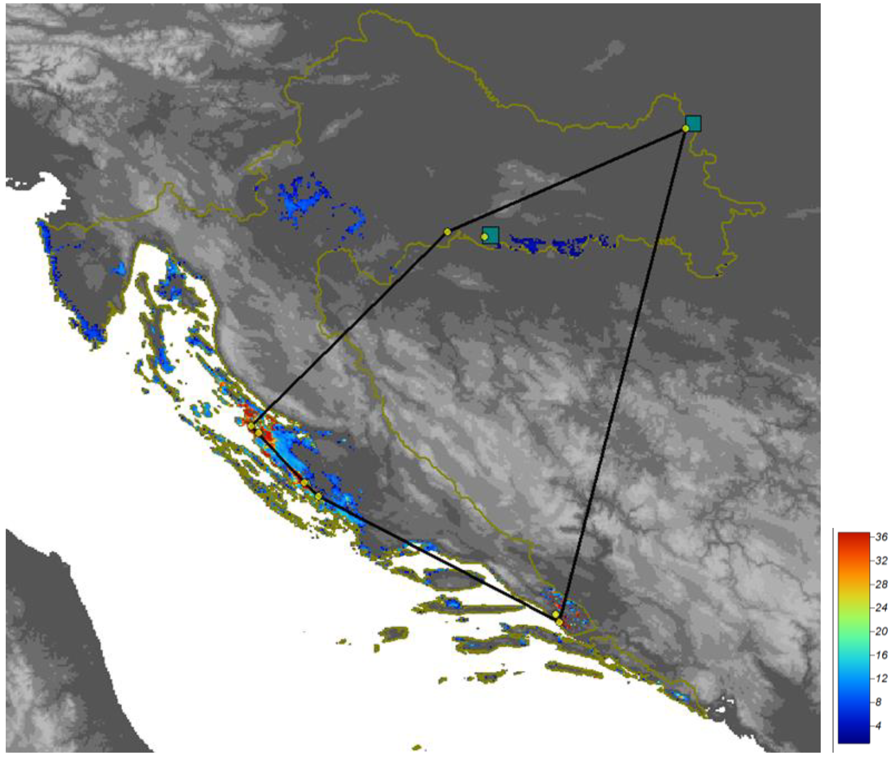
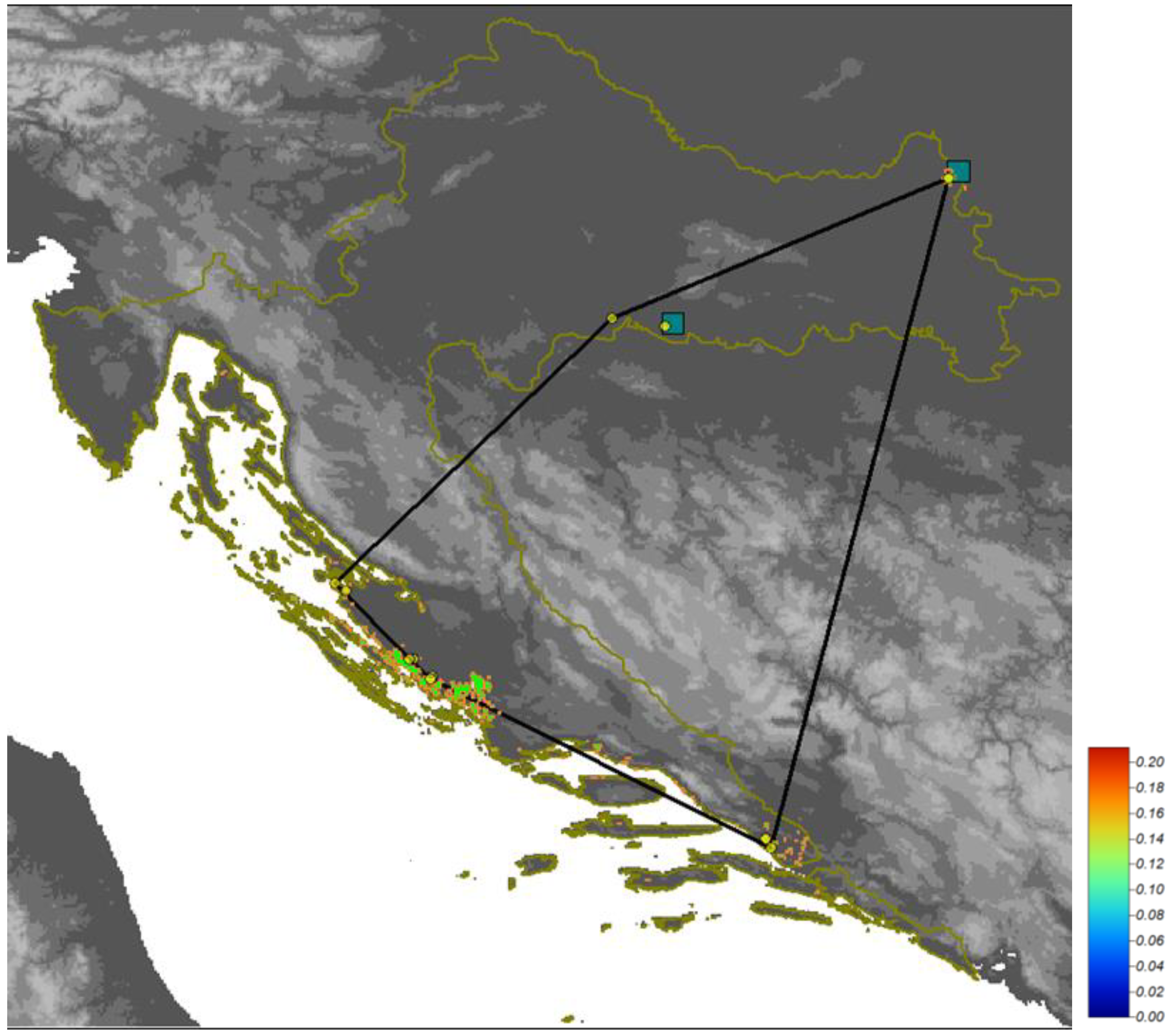
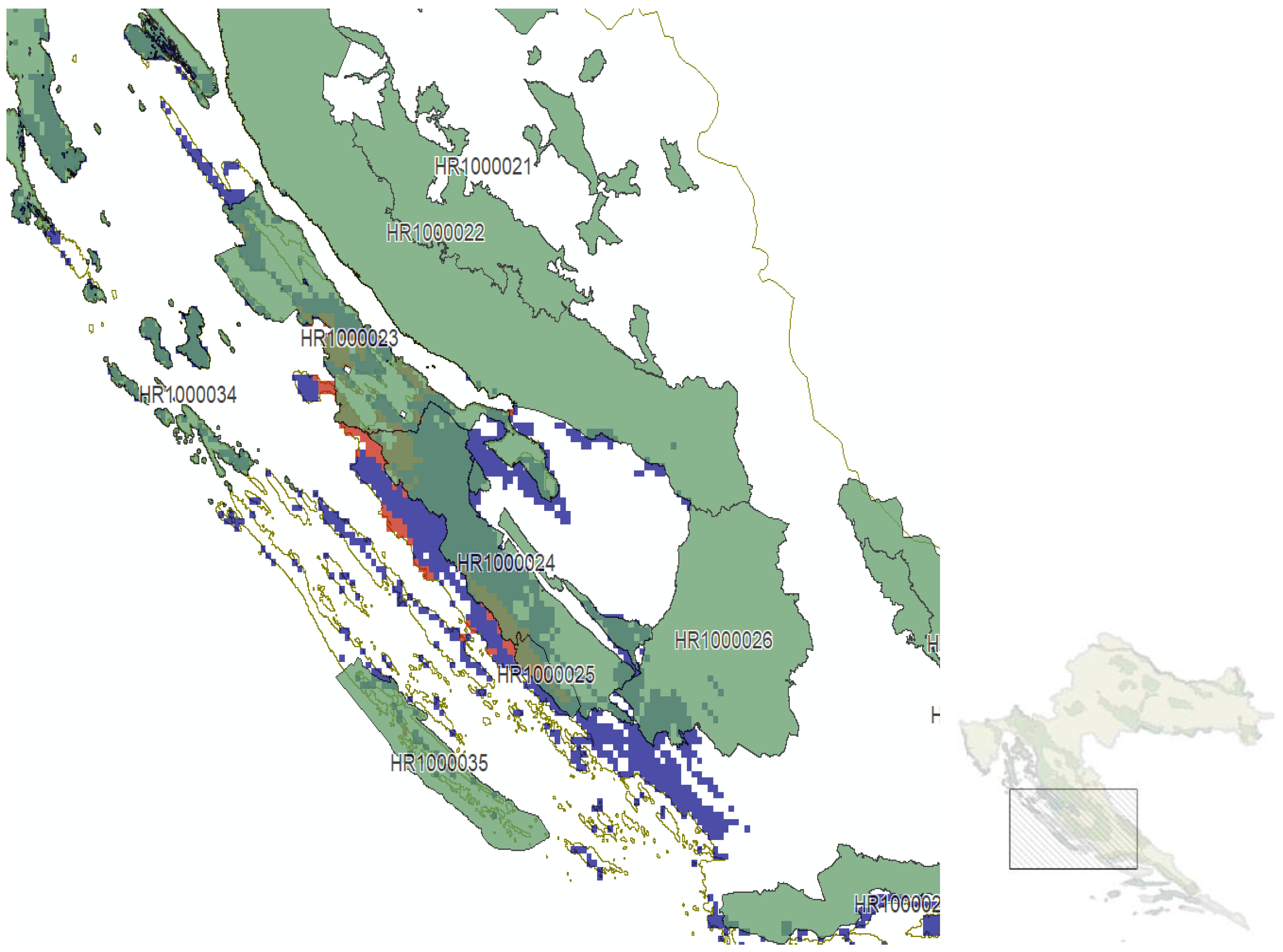
To assess breeding suitability at the national scale, a Random Forest (RF) classification model was employed. The RF model identified 437 1 × 1 km grid cells as suitable for breeding, suggesting a total breeding area of 437 km2. Variable importance from the RF model showed that top predictors included digital elevation (DEM; importance: 0.01715), a maximum temperature of the warmest month (BIO_5; 0.01437), and the extent of wetland habitat (AGG_A4; 0.01173), along with several other temperature and precipitation-related bioclimatic variables (see Table 2 below). Spatial models provided valorization of Croatian territory for M. pygmaeus (Figure 2, Figure 3 and Figure 4; Table 2), completely randomly selected species for presenting results, allowing post-hoc evaluation and ranking of protected areas for the species and expert-based estimation of the population size.
Interestingly, the models predict suitable breeding habitats for the species along the entire Istrian coast and other northern parts of Croatia. However, no breeding records exist for these areas. For this and many other species, the models often identify ecologically similar areas to those where the species has been observed.
There may be multiple reasons why the species has not been recorded in certain areas: the species may not actually occur in these regions because of an environmental variable not included in the model. The limiting factor may not necessarily be an environmental variable but rather a consequence of land management practices. Constraints could include insufficient habitat size to meet the species’ needs and increased disturbances due to human activities such as habitat disruption or hunting.
A large number of environmental factors that restrict species’ settlement—especially for species requiring complex habitat combinations over large areas—cannot be easily mapped or adequately incorporated into spatial models. This is particularly true for variables describing human activities in the landscape and physical barriers such as fences, which may significantly impact species distribution.
The post-hoc analytical approach differed substantially across bird guilds and ecological profiles; therefore, we do not present the full process for each species here. In brief, for each species/population, we evaluated habitat suitability across Croatian territory, identified key environmental variables correlated with distribution, and compared suitability scores within and outside protected areas. Final estimations of population sizes—both within protected areas and nationwide—were made using expert knowledge and interpolated species densities applied to areas classified as suitable by the RF model.
In the case of M. pygmaeus, the results (Figure 2) show that the Croatian population is neither marginal nor limited by major climate or land cover constraints. When comparing models, both Maxent and RF showed general agreement at the national scale, although differences emerge in marginal areas. Maxent, which provides a continuous habitat suitability index (ranging from 0 to 100), tends to highlight broader gradients of suitability, while the RF model outputs a binary classification (0 or 1), categorizing each grid cell as either suitable or unsuitable, resulting in sharper habitat boundaries.
Notably, the RF model excluded several central and eastern areas of Croatia that were considered potentially suitable by Maxent. This discrepancy emphasizes the difference in how both algorithms define suitability thresholds. Furthermore, as shown in Figure 3 and Figure 4, which display a convex hull around national occurrence data from the past 25 years, many areas predicted as suitable breeding habitats lack any observational records. This gap may be due to unmodeled variables, such as local land use practices, habitat fragmentation, or the presence of physical barriers, all of which can significantly affect the actual occupancy of predicted suitable areas.
At the national scale, the habitat suitability for M. pygmaeus was modeled using both Maxent and Random Forest (RF) algorithms. Maxent, using global GBIF data, predicted coastal and eastern inland regions of Croatia as suitable breeding habitats. Interestingly, Maxent also identified northern and Istrian coastal zones as highly suitable, although no breeding records exist from these areas. Such an overprediction may be due to unmodeled constraints such as human disturbance, land management practices, or fine-scale habitat structure.
To complement Maxent and to produce a binary habitat classification, we applied a Random Forest (RF) classification model using the randomForest package in R. The model was trained on the dataset data_for_RF using the formula index~., with 1000 trees and the na.roughfix method for missing values. The RF algorithm identified 437 1 × 1 km grid cells as suitable breeding habitats, corresponding to a national breeding area of 437 km2.
The most influential variables in the RF model were DEM_1k (elevation): 0.01715; bio5_16 (max temperature of the warmest month): 0.01437; agg_A4 (area of inland water and wetland habitats): 0.01173. Other contributing variables included temperature seasonality, precipitation of the warmest quarter, and additional habitat area indicators (see Table 3).
The confusion matrix indicated perfect classification of absences (50/50) but lower sensitivity for presences, with 10 out of 14 known breeding sites correctly classified (classification error for presences = 28.6%). This result suggests some caution when interpreting binary predictions, especially in fragmented or marginal habitats.
Post-Hoc Evaluation and Population Estimation
For all species in this study, including M. pygmaeus, the modeling results were further refined through expert-driven post-hoc evaluations. These involved:
Quantification and ranking of environmental variables correlated with species presence, comparison of protected area effectiveness for habitat provision,
Estimation of occupied territories and interpolation of population size across suitable habitat patches.
In the case of M. pygmaeus, it is clear from Figure 2 that the Croatian breeding population is not climatically or geographically marginal. However, Figure 3 and Figure 4, which include a convex hull of national presence records from the past 25 years, show that many potentially suitable areas lack any confirmed observations. This discrepancy reinforces the need for expert validation, especially for species with patchy distributions or specific ecological constraints.
The combined modeling approach, integrating spatial algorithms and expert post-hoc assessments, provides a robust framework for evaluating population sizes and habitat values, even when systematic data collection is limited. By using species with differing habitat complexity and ecological specificity, this approach ensures broader applicability across bird conservation planning.
The approach to post-hoc analyses is significantly different for different bird guilds, so we are not presenting the process made for each bird species in regard to the guild and ecological specificity of the species. In summary, for each species/population, an evaluation of Croatian territory was performed, and quantification and ranking of environmental variables were performed for those that have the highest correlation with detected species spatial distributions. Additionally, a comparison of protected areas for suitability for the species (Table 4), estimation of occupied territories, and estimation of the population size for the protected area and overall Croatian territory was given by adequate interpolating of species densities at suitable habitats obtained with the classification RF algorithm.
In the case of the presented species, M. pygmaeus, Figure 2 shows that the Croatian population is not in any way a marginal population limited by climate or land cover variables. At a national scale, the two models correspond, but the differences are mostly visible in the less suitable areas for the species. The classification type RF algorithm did not predict the central and eastern part of Croatia as suitable areas. The reason for this is that the Maxent algorithm is an algorithm that provides a suitability index in the range of 0–100, but the classification type RF algorithm produced a binary variable (0, 1), so each pixel can be either suitable or unsuitable for the population and clear cut-offs are made. Looking at Figure 3 and Figure 4, where we presented convex hull around national presence data from the last 25 years, it is visible that for the majority of potentially suitable breeding habitats for the species, there are no observations of the species whatsoever.

4. Discussion

Species distribution models (SDMs) are indispensable tools for identifying habitat preferences and informing conservation strategies, particularly in regions where standardized biodiversity data are lacking. In this study, we applied two machine learning approaches—Maxent and Random Forest (RF)—to predict the breeding distribution of birds in Croatia, with a case focus on M. pygmaeus. Despite the inherent limitations of presence-only datasets, both models provided ecologically meaningful insights that can support biodiversity planning at national and local scales.
The Random Forest model for M. pygmaeus identified key environmental predictors aligned with the species’ known ecological niche. Elevation (DEM_1k), the maximum temperature of the warmest month (bio5), and proximity to inland water and wetland habitats emerged as the most important variables. These findings are consistent with the species’ preference for lowland freshwater wetlands, confirming the ecological plausibility of the model outputs. The Maxent model, by producing a continuous habitat suitability index, offered finer resolution insights into habitat quality within protected areas, while the RF model’s binary classification was effective in delineating areas suitable for breeding.
The confusion matrix from the RF model indicated high accuracy for absence predictions, while true presences were slightly underrepresented, with a classification error of 28.6% for the presence class. This discrepancy highlights a broader challenge in SDM application—model performance may be skewed when presence data are limited or spatially biased, as is often the case with citizen science datasets [12,42].
A major limitation of biodiversity research in Croatia is the absence of systematically collected presence–absence data. Current databases are largely derived from opportunistic observations, often concentrated in protected areas, which introduce spatial bias. Such data are not ideally suited for parametric modeling approaches such as Generalized Linear Models (GLMs) or Generalized Additive Models (GAMs), necessitating the use of machine learning algorithms that can accommodate presence-only data, such as Maxent and RF (which internally generate pseudo-absences) [11,12].
To address these limitations, we incorporated expert validation into the modeling process. Expert knowledge was used to refine model outputs and ensure ecological credibility, particularly in cases where species distributions were poorly represented by these data. This integration of expert judgment is essential for generating reliable models under data-limited conditions and helps bridge the gap between statistical predictions and real-world ecological patterns.
Earth observation data derived from remote sensing technologies were fundamental to our modeling approach. Variables such as temperature, precipitation, land cover, and vegetation indices were sourced from platforms such as Sentinel, Landsat, and the Copernicus Climate Data Store. These datasets allow for consistent, high-resolution environmental characterization across large geographic extents, enabling SDMs to operate effectively even when field-based measurements are sparse or unevenly distributed [3,43].
In particular, remote sensing enables monitoring of dynamic environmental processes—such as vegetation seasonality and surface water availability—which are crucial for species such as M. pygmaeus that depend on aquatic habitats. The integration of such data strengthens the predictive power of SDMs and supports the assessment of habitat changes over time, including those driven by climate change or anthropogenic disturbance [11].
While remote sensing and expert input can partially compensate for data gaps, the lack of standardized ecological monitoring remains a critical barrier to biodiversity modeling in Croatia. The absence of systematic sampling protocols limits the ability to model species’ ecological niches accurately and to validate model predictions against independent datasets.
Improving national biodiversity datasets through the implementation of standardized monitoring protocols would significantly enhance the utility of SDMs [12]. Aligning data collection efforts with international best practices—such as the Global Biodiversity Observation Network (GEO BON) or Essential Biodiversity Variables (EBVs)—would enable Croatia to improve both the quality of ecological research and the effectiveness of conservation policy.
Future developments in remote sensing, including higher spatial resolution, increased temporal frequency, and integration with citizen science platforms, may offer new opportunities to improve species distribution models. Technologies such as unmanned aerial vehicles (UAVs) and real-time environmental sensors could provide novel data sources to further support habitat assessments and dynamic SDMs.
Despite the inherent limitations in data quality, this study demonstrates that the combination of machine learning algorithms, Earth observation data, and expert input can yield reliable models for biodiversity assessment. These models can inform conservation planning by identifying key habitats, estimating population distributions, and guiding resource allocation. For species of conservation concern, such as M. pygmaeus, SDMs can support targeted monitoring efforts and proactive habitat management.
However, for SDMs to reach their full potential, investments in biological data infrastructure are urgently needed. The adoption of systematic, long-term biodiversity monitoring programs will be critical for enhancing the accuracy, transparency, and applicability of predictive ecological models in Croatia and similar data-poor regions.

5. Conclusions

This study demonstrates the utility of machine learning–based species distribution models (SDMs) in ecological research and conservation planning, even in data-limited contexts such as Croatia. By applying Maxent and Random Forest algorithms to model the breeding distribution of M. pygmaeus, we were able to identify key environmental variables—such as temperature, wetland coverage, and elevation—that define suitable habitats for this species at the national scale.
Despite the limitations associated with presence-only data and opportunistic observations, our approach—supplemented by expert input and remotely sensed environmental variables—yielded ecologically meaningful predictions. The integration of Earth observation data proved critical for enhancing model performance and enabling spatially explicit assessments of habitat suitability, particularly in areas lacking ground-based biodiversity monitoring.
Our findings underscore the urgent need to improve biodiversity data collection practices in Croatia. Systematic, high-quality presence–absence data are essential to validate and refine predictive models and to align national conservation efforts with global best practices. Moving forward, the adoption of standardized monitoring protocols, coupled with ongoing advancements in remote sensing technology, will be essential for supporting robust, data-driven biodiversity management.
In conclusion, the combined use of SDMs, remote sensing, and expert knowledge offers a practical and effective pathway for improving species conservation outcomes in regions with limited ecological datasets. Such an approach provides a scalable framework for assessing habitat suitability, guiding field surveys, and prioritizing conservation interventions in support of biodiversity preservation.

Author Contributions

Validation, L.T.T.; Formal analysis, A.R.; Data curation, S.K.; Writing—original draft, A.R. All authors have read and agreed to the published version of the manuscript.

Funding

This research received no external funding.

Institutional Review Board Statement

Not applicable.

Data Availability Statement

The data that support the findings of this study are not publicly available due to restrictions imposed by third-party ownership. Access to the data is therefore not possible through the authors.

Conflicts of Interest

The authors declare no conflict of interest.

References

  1. Elith, J.; Leathwick, J.R. Species distribution models: Ecological explanation and prediction across space and time. Annu. Rev. Ecol. Evol. Syst. 2009, 40, 677–697. [Google Scholar] [CrossRef]
  2. Gallien, L.; Münkemüller, T.; Albert, C.H.; Boulangeat, I.; Thuiller, W. Predicting potential distributions of invasive species: Where to go from here? Divers. Distrib. 2010, 16, 331–342. [Google Scholar] [CrossRef]
  3. Bannari, A.; Huete, A.R.; Morin, D.; Bonn, F. A review of vegetation indices. Remote Sens. Rev. 1995, 13, 95–120. [Google Scholar] [CrossRef]
  4. Peterson, A.T.; Soberón, J.; Pearson, R.G.; Anderson, R.P.; Martínez-Meyer, E.; Nakamura, M.; Araújo, M.B. Ecological Niches and Geographic Distributions; Princeton University Press: Princeton, NJ, USA, 2011. [Google Scholar] [CrossRef]
  5. Guisan, A.; Thuiller, W. Predicting species distribution: Offering more than simple habitat models. Ecol. Lett. 2005, 8, 993–1009. [Google Scholar] [CrossRef]
  6. Broennimann, O.; Treier, U.A.; Müller-Schärer, H.; Thuiller, W.; Peterson, A.T.; Guisan, A. Analyzing niche dynamics during biological invasions. Ecol. Lett. 2007, 10, 701–719. [Google Scholar] [CrossRef]
  7. Stein, A.; Gerstner, K.; Kreft, H. Environmental heterogeneity as a universal driver of species richness across taxa, biomes and spatial scales. Ecol. Lett. 2014, 17, 866–880. [Google Scholar] [CrossRef]
  8. Petersen, C. Integrating remote sensing data into species distribution models. Ecography 2013, 36, 789–800. [Google Scholar]
  9. Merow, C.; Smith, M.J.; Silander, J.A., Jr. A practical guide to MaxEnt for modeling species’ distributions: What it does, and why inputs and settings matter. Ecography 2013, 36, 1058–1069. [Google Scholar] [CrossRef]
  10. Phillips, S.J.; Anderson, R.P.; Schapire, R.E. Maximum entropy modeling of species geographic distributions. Ecol. Model. 2006, 190, 231–259. [Google Scholar] [CrossRef]
  11. Elith, J.; Leathwick, J.R.; Hastie, T. A working guide to boosted regression trees. J. Anim. Ecol. 2011, 77, 802–813. [Google Scholar] [CrossRef]
  12. He, K.S.; Bradley, B.A.; Cord, A.F.; Rocchini, D.; Tuanmu, M.N.; Schmidtlein, S.; Turner, W.; Wegmann, M.; Pettorelli, N. Integrating remote sensing data into species distribution models. Ecography 2013, 36, 789–800. [Google Scholar]
  13. Franklin, J. Mapping Species Distributions: Spatial Inference and Prediction; Cambridge University Press: Cambridge, UK, 2010. [Google Scholar] [CrossRef]
  14. Thomas, C.D.; Cameron, A.; Green, R.E.; Bakkenes, M.; Beaumont, L.J.; Collingham, Y.C.; Erasmus, B.F.N.; Ferreira de Siqueira, M.; Grainger, A.; Hannah, L.; et al. Extinction risk from climate change. Nature 2004, 427, 145–148. [Google Scholar] [CrossRef] [PubMed]
  15. Pearson, R.G.; Dawson, T.P. Predicting the impacts of climate change on the distribution of species: Are bioclimate envelope models useful? Glob. Ecol. Biogeogr. 2003, 12, 361–371. [Google Scholar] [CrossRef]
  16. Bueno de Mesquita, C.P.; King, A.J.; Schmidt, S.K.; Farrer, E.C.; Suding, K.N. Incorporating biotic factors in species distribution modelling: Are interactions with soil microbes important? Ecography 2016, 39, 970–980. [Google Scholar] [CrossRef]
  17. Zhang, L. Use of remote sensing in biodiversity monitoring and ecosystem management. Biodivers. Conserv. 2019, 28, 2225–2237. [Google Scholar]
  18. Hirzel, A.H.; Le Lay, G. Habitat suitability modelling and niche theory. J. Appl. Ecol. 2008, 45, 1372–1381. [Google Scholar] [CrossRef]
  19. GBIF. Global Biodiversity Information Facility. Available online: https://www.gbif.org/ (accessed on 15 December 2024).
  20. Kapelj, S.; Radović, A.; Zec, M.; Mihelič, T.; Mikac, S.; Maslać Mikulec, M.; Patčev, E.; Dender, D.; Taylor, L.; Mikuška, T.; et al. Završno Izvješće Usluge Definiranja SMART Ciljeva Očuvanja i Osnovnih Mjera Očuvanja Ciljnih Vrsta i Stanišnih Tipova—Grupa 5: Definiranje Ciljeva i Mjera Očuvanja za Nedovoljno Poznate Prste Ptica; Udruga BIOM, Geonatura, DOPPS: Zagreb, Croatia, 2023; p. 36. [Google Scholar]
  21. European Environmental Agency. Environmental Datasets. Available online: https://www.eea.europa.eu/en/datahub/datahubitem-view/3c362237-daa4-45e2-8c16-aaadfb1a003b (accessed on 15 May 2023).
  22. EEA, EU_DEM Ver 1.1., 2016. Available online: https://www.eea.europa.eu/en/datahub/datahubitem-view/d08852bc-7b5f-4835-a776-08362e2fbf4b (accessed on 10 July 2023).
  23. Habitat Map of Croatia. Available online: https://www.haop.hr/hr/baze-i-portali/karta-stanista-rh-2004 (accessed on 10 July 2023).
  24. Non-Forest Habitat Map of Croatia. Available online: https://www.haop.hr/hr/baze-i-portali/karta-kopnenih-nesumskih-stanista-republike-hrvatske-2016 (accessed on 16 June 2023).
  25. Zenodo. Copernicus Land Cover Data. Available online: https://zenodo.org/communities/copernicus-land-cover/ (accessed on 10 June 2023).
  26. Riitters, K.H.; O’Neill, R.V.; Hunsaker, C.T.; Wickham, J.D.; Yankee, D.H.; Timmins, S.P.; Jones, K.B.; Jackson, B.L. A factor analysis of landscape pattern and structure metrics. Landsc. Ecol. 1995, 10, 23–40. [Google Scholar] [CrossRef]
  27. Hesselbarth, M.H.K.; Sciaini, M.; With, K.A.; Wiegand, K.; Nowosad, J. landscapemetrics: An open-source R tool to calculate landscape metrics. Ecography 2019, 42, 1648–1657. [Google Scholar] [CrossRef]
  28. Hijmans, R.J.; Barbosa, M.; Ghosh, A.; Mandel, A. _geodata: Download Geographic Data_. R package version 0.5–9. 2023. Available online: https://CRAN.R-project.org/package=geodata (accessed on 10 June 2023).
  29. R Core Team. _R: A Language and Environment for Statistical Computing_; R Foundation for Statistical Computing: Vienna, Austria; Available online: https://www.R-project.org/ (accessed on 10 June 2023).
  30. Phillips, S.J.; Dudík, M. Understanding and applying MaxEnt, a machine-learning approach for species distribution modeling. J. Biogeogr. 2008, 35, 1–11. [Google Scholar]
  31. Liaw, A.; Wiener, M. Classification and Regression by RandomForest. R News 2002, 2, 18–22. [Google Scholar]
  32. Schauberger, P.; Walker, A. _openxlsx: Read, Write and Edit xlsx Files_. R package version 4.2.5.2. Available online: https://CRAN.R-project.org/package=openxlsx (accessed on 10 June 2023).
  33. Pebesma, E. Simple features for R: Standardized support for spatial vector data. R J. 2018, 10, 1–8. [Google Scholar] [CrossRef]
  34. Pebesma, E.; Bivand, R. Spatial Data Science: With Applications in R, 1st ed.; Chapman and Hall/CRC: Boca Raton, FL, USA, 2023. [Google Scholar] [CrossRef]
  35. Aiello-Lammens, M.E.; Boria, R.A.; Radosavljevic, A.; Vilela, B.; Anderson, R.P. spThin: An R package for spatial thinning of species occurrence records for use in ecological niche models. Ecography 2015, 38, 541–545. Available online: https://onlinelibrary.wiley.com/doi/10.1111/ecog.01132.(accessed on 15 June 2023)
  36. Hijmans, R.; Phillips, S.; Leathwick, J.; Elith, J. _dismo: Species Distribution Modeling_. R Package Version 1.3–16, 2024. Available online: https://CRAN.R-project.org/package=dismo (accessed on 15 June 2023).
  37. Bivand, R.; Rundel, C. rgeos: Interface to Geometry Engine—Open Source (‘GEOS’); R Package Version 0.6-2. Available online: https://CRAN.R-project.org/package=rgeos (accessed on 15 June 2023).
  38. Kass, J.M.; Pinilla-Buitrago, G.E.; Paz, A.; Johnson, B.A.; Grisales-Betancur, V.; Meenan, S.I.; Attali, D.; Broennimann, O.; Galante, P.J.; Maitner, B.S.; et al. wallace 2: A shiny app for modeling species niches and distributions redesigned to facilitate expansion via module contributions. Ecography 2023, 2023, e06547. [Google Scholar] [CrossRef]
  39. Hijmans, R. Terra: Spatial Data Analysis; R Package Version 1.7–29. Available online: https://CRAN.R-project.org/package=terra (accessed on 15 June 2023).
  40. Hijmans, R. _raster: Geographic Data Analysis and Modeling_. R Package Version 3.6–26, 2023. Available online: https://CRAN.R-project.org/package=raster (accessed on 15 June 2023).
  41. Kass, J.M.; Muscarella, R.; Galante, P.J.; Bohl, C.L.; Pinilla-Buitrago, G.E.; Boria, R.A.; Soley-Guardia, M.; Anderson, R.P. ENMeval 2.0: Redesigned for customizable and reproducible modeling of species’ niches and distributions. Methods Ecol. Evol. 2021, 12, 1602–1608. [Google Scholar] [CrossRef]
  42. Long, A.M.; Pierce, B.L.; Anderson, A.D.; Skow, K.L.; Smith, A.; Lopez, R.R. Integrating citizen science and remotely sensed data to help inform time-sensitive policy decisions for species of conservation concern. Biol. Conserv. 2019, 237, 463–469. [Google Scholar] [CrossRef]
  43. Valavi, R.; Guillera-Arroita, G.; Lahoz-Monfort, J.J.; Elith, J. Predictive performance of presence-only species distribution models: A benchmark study with reproducible code. Ecol. Monogr. 2022, 92, 1. [Google Scholar] [CrossRef]
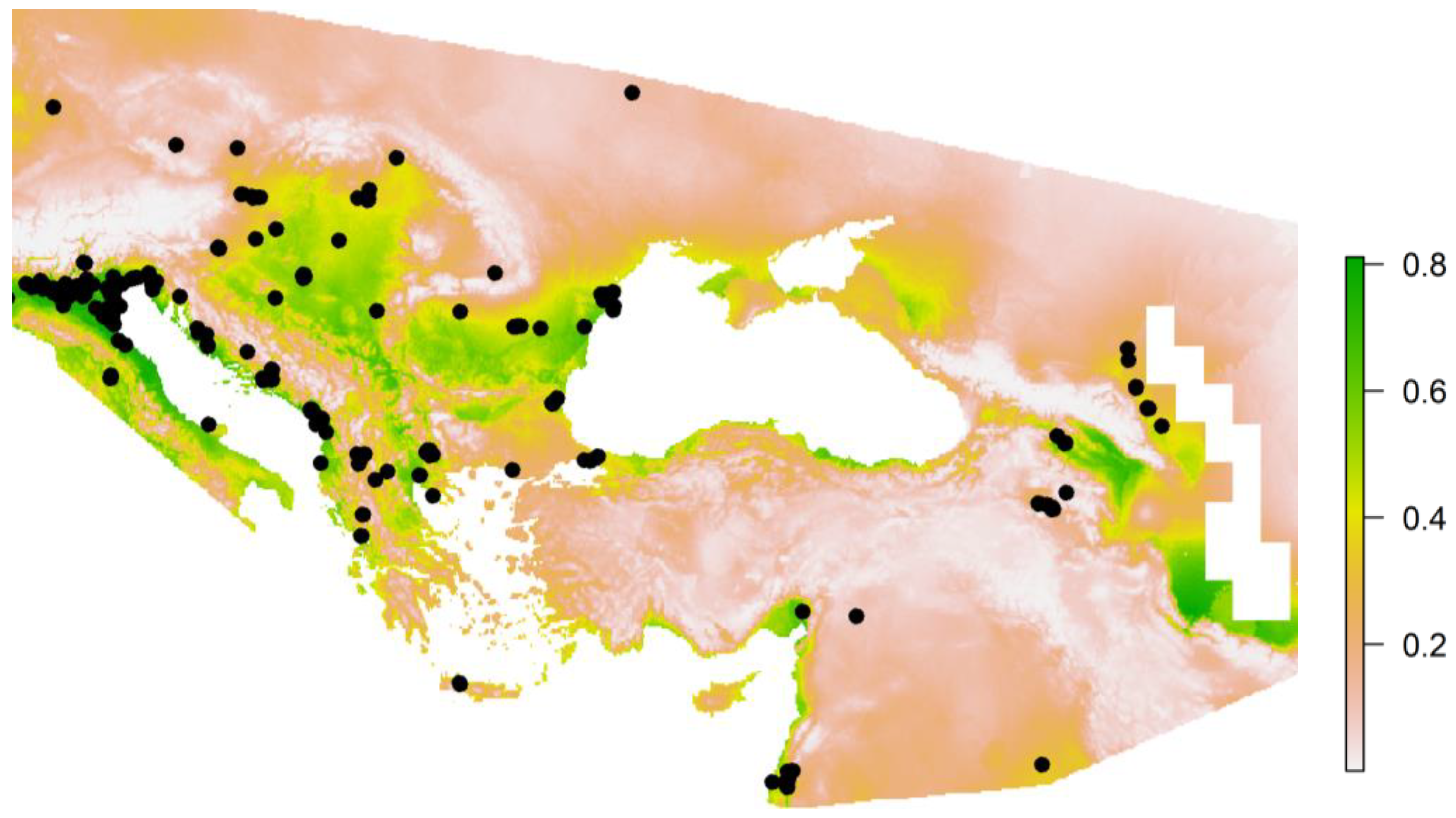
Figure 1. Regional valorization of space for breeding population of the species M. pygmaeus using Maxent modeling and GBIF data (black dots). Greener colors in the figure represent higher suitability for the breeding population of the species.
Diversity 17 00399 g001
Figure 2. Habitat suitability, national valorization of space for breeding population of the species M. pygmaeus using Maxent modeling using national data not older than 25 years Black polygon is convex hull around data. Green squares are 10 km by 10 km squares with at least one presence of the species from the last 5 years. Red–orange colors represent the most suitable area for the breeding population of the species.
Diversity 17 00399 g002
Figure 3. Detected breeding area and national valorization for the breeding population of the species M. pygmaeus using a Random Forest classification algorithm and national data not older than 25 years. The black polygon is a convex hull around data. Green squares are 10 km by 10 km squares with at least one presence of the species from the last 5 years. Red–orange colors represent the most suitable area for the breeding population of the species.
Diversity 17 00399 g003
Figure 4. Example of final lassification of Maxent algorithm habitat suitability result at national scale for breeding population of M. pygmaeus; zoom at North Dalmatiathe square.
Diversity 17 00399 g004
Table 1. List of bird species and ecological groups of bird species included in this work/presented only M. pygmaeus as an example.
Ecological GroupSpecies
Woodpeckers and PicidsDendrocopos leucotos, Dendrocopos major, Dendrocopos syriacus, Dryobates minor, Dryocopus martius, Leiopicus medius, Picoides tridactylus, Picus canus, Picus viridis
Birds of Prey (Raptors)Circaetus gallicus, Accipiter brevipes, Accipiter gentilis, Tachyspiza nisus, Aquila fasciata, Clanga pomarina, Buteo buteo, Falco subbuteo, Falco vespertinus, Falco biarmicus, Falco columbarius, Hieraaetus pennatus, Pernis apivorus, Circus cyaneus, Milvus migrans
Game BirdsAlectoris graeca, Tetrao urogallus, Bonasa bonasia
Nocturnal BirdsCaprimulgus europaeus, Aegolius funereus, Glaucidium passerinum
Herons, Egrets, and AlliesArdea alba, Ardea cinerea, Ardea purpurea, Ardeola ralloides, Egretta garzetta, Nycticorax nycticorax
Spoonbills and IbisesPlatalea leucorodia, Plegadis falcinellus
CormorantsMicrocarbo pygmaeus, Phalacrocorax carbo sinensis
Terns and GullsChlidonias hybrida, Chlidonias niger, Thalasseus sandvicensis, Hydrocoloeus minutus, Larus melanocephalus, Larus ridibundus
Rails and CrakesFulica atra, Gallinula chloropus, Porzana porzana, Rallus aquaticus, Zapornia parva, Zapornia pusilla
Ducks, Geese, and SwansAnas acuta, Anas crecca, Anas platyrhynchos, Anser albifrons albifrons, Anser anser, Anser fabalis rossicus, Aythya ferina, Aythya fuligula, Aythya nyroca, Bucephala clangula, Cygnus olor, Mareca penelope, Mareca strepera, Netta rufina, Spatula clypeata, Spatula querquedula
GrebesPodiceps cristatus, Podiceps grisegena, Podiceps nigricollis, Tachybaptus ruficollis
PasserinesAlcedo atthis, Riparia riparia, Acrocephalus arundinaceus, Acrocephalus melanopogon, Acrocephalus schoenobaenus, Acrocephalus scirpaceus, Cettia cetti, Cisticola juncidis, Emberiza schoeniclus, Locustella fluviatilis, Locustella luscinioides, Panurus biarmicus, Remiz pendulinus, Hippolais olivetorum
Shorebirds and WadersActitis hypoleucos, Calidris alpina, Calidris pugnax, Charadrius alexandrinus, Charadrius dubius, Grus grus, Haematopus ostralegus, Himantopus himantopus, Limosa limosa, Numenius arquata arquata, Numenius phaeopus, Pluvialis squatarola, Recurvirostra avosetta, Tringa erythropus, Tringa glareola, Tringa nebularia
Large WaterbirdsBotaurus stellaris, Ixobrychus minutus
Table 2. List of environmental variables that influence the spatial distribution of the breeding population of M. pygmaeus at a national scale.
VariableDescriptionAbs Significance
DEMDigital elevation model0.01715
BIO_5Max Temperature of Warmest Month0.01437
AGG_A4Area of habitat A1 (element of inland surface water and wetlands)0.01173
BIO_9Mean Temperature of Driest Quarter0.00879
BIO_18Precipitation of Warmest Quarter0.00845
BIO_1Annual Mean Temperature0.00683
BIO_3Isothermality0.00609
BIO_10Mean Temperature of Warmest Quarter0.00554
AGG_A1Area of habitat A4 (element of inland surface water and wetlands)0.00548
Table 3. The condensed list of variables prepared and used in different geographical contexts.
CategoryVariable NameDescription
Morphometric VariablesDigital Elevation Model (DEM)Surface elevation model
Wetness Index (WI)Potential water accumulation index
SlopeTerrain slope
Habitat VariablesHabitat Type PresencePresence (1) or absence (0) of habitat type at reference grid
Habitat Type AreaArea of each habitat type at 1 km reference grid
Aggregated Habitat TypesSpatial aggregation of habitat types up to 2nd level of national classification scheme (e.g., agg_A1, agg_A2, agg_B12, etc.)
Habitat Heterogeneity VariablesAveraged ConnectivityAverage connectivity between habitat fragments
ConnectivityConnectivity between habitat fragments
DiversityDegree of habitat heterogeneity
Number of CategoriesNumber of different land cover categories per grid
Bioclimatic Variables (WorldClim BIOCLIM)BIO1—Annual Mean TemperatureAverage annual temperature
BIO2—Mean Diurnal RangeMean difference between daily max and min temperatures
BIO3—IsothermalityRatio of mean diurnal range to the annual temperature range
BIO4—Temperature SeasonalityVariation in temperature throughout the year
BIO5—Max Temperature of Warmest MonthMaximum temperature of the hottest month
BIO6—Min Temperature of Coldest MonthMinimum temperature of the coldest month
BIO7—Temperature Annual RangeDifference between BIO5 and BIO6
BIO8—Mean Temperature of Wettest QuarterMean temperature during the wettest 3-month period
BIO9—Mean Temperature of Driest QuarterMean temperature during the driest 3-month period
BIO10—Mean Temperature of Warmest QuarterMean temperature during the warmest 3-month period
BIO11—Mean Temperature of Coldest QuarterMean temperature during the coldest 3-month period
BIO12—Annual PrecipitationTotal annual precipitation
BIO13—Precipitation of Wettest MonthPrecipitation in the wettest month
BIO14—Precipitation of Driest MonthPrecipitation in the driest month
BIO15—Precipitation SeasonalityVariation in monthly precipitation levels
BIO16—Precipitation of Wettest QuarterTotal precipitation in the wettest 3-month period
BIO17—Precipitation of Driest QuarterTotal precipitation in the driest 3-month period
BIO18—Precipitation of Warmest QuarterTotal precipitation in the warmest 3-month period
BIO19—Precipitation of Coldest QuarterTotal precipitation in the coldest 3-month period
Land Cover Categories (ESA LC 2021)Tree CoverPercentage of tree cover
ShrublandPercentage of shrub cover
GrasslandPercentage of grassland cover
CroplandPercentage of agricultural land
Built-up AreasPercentage of artificial surfaces
Bare/Sparse VegetationPercentage of barren land
Snow and IcePercentage of snow and ice cover
Permanent Water BodiesPercentage of surface covered by water
Herbaceous WetlandPercentage of wetland cover
MangrovePercentage of mangrove cover
Moss and LichenPercentage of moss and lichen cover
Table 4. Comparison among protected areas for breeding population of M. pygmaeus based on results of Maxent algorithm.
Sort Site IDCount/Area of the SiteNMINMAXMEAN
040,139,618177,53616210.32
1228,4840
246,9230
331,817224271210.73
4204,609164123111.38
597,5780
614,4860
745,3770
824,6640
95883512615129.41
1021,7680
1161,25227,45216224.56
1210,7520
1323,4050
1488,764789112910.12
1567,10947,89616217.57
1669,1040
1787,7990
1830,2390
1938,4232354599.95
2047,33414031126.92
2114,5500
2220,203600395.66
2320,5710
24390
2538,4100
2685,75884551298.25
2714,594707611910.72
2813,4640
2918,2673990195.96
3019281961117.98
3139,97314,091141.97
3235,83917,4171106.04
33123,4541198142.41
3416680
3523,7900
3629,28728423349.33
3724,891597116232.36
38120,92733,5421328.69
Disclaimer/Publisher’s Note: The statements, opinions and data contained in all publications are solely those of the individual author(s) and contributor(s) and not of MDPI and/or the editor(s). MDPI and/or the editor(s) disclaim responsibility for any injury to people or property resulting from any ideas, methods, instructions or products referred to in the content.