Article

Seasonal Dynamics of Fisheries and Crustacean Communities in the Offshore of the Zhoushan Archipelago Seas: A Size Spectrum Analysis

1
Zhejiang Marine Fisheries Institute, Zhoushan 316021, China
2
Scientific Observing and Experimental Station of Fishery Resources for Key Fishing Grounds, Ministry of Agriculture and Rural Affairs, Zhoushan 316021, China
3
School of Fisheries, Zhejiang Ocean University, Zhoushan 316022, China
*
Author to whom correspondence should be addressed.
Diversity 2025, 17(11), 744; https://doi.org/10.3390/d17110744
Submission received: 13 September 2025 / Revised: 18 October 2025 / Accepted: 19 October 2025 / Published: 23 October 2025
(This article belongs to the Special Issue Dynamics of Marine Communities—Second Edition)

Abstract

Understanding the seasonal dynamics of the fisheries and crustacean communities are of crucial ecological significance. To investigate the structural characteristics of these communities and their seasonal dynamics in the offshore of the Zhoushan Archipelago Seas, China, this study conducted a four seasons’ trawl survey to collect fisheries data in spring, summer, autumn, and winter of 2022. A normalized abundance size spectrum approach was applied to investigate the seasonal variation in regressed parameters (slope and intercept) for fish-only and fish-plus-crustacean communities. Our study found that average values of the slope of the size spectrum for fish and fish-plus-crustacean were −1.36 and −1.53, respectively; the overall adding effect with crustaceans in all seasons was more negative (a steeper slope). The results also showed that the adding effect of crustaceans in the fisheries communities were season-specific and region-specific. Temporally, adding crustaceans into fisheries communities contributed to more/less negative slopes in temperate/warm seasons, respectively. Regionally, the inclusion of crustaceans induced a reverse distribution pattern (nearshore–offshore) for fish abundance, as well as the re-scaled intercept, which could indicate the abundance in all seasons except in summer. It was assumed that although fish dominated the overall community structure, crustaceans contributed a compensatory effect by regulating the size distribution across trophic levels. This study provides valuable insights for the dynamic assessment and scientific management of fisheries and crustacean resources in the whole ecosystem.

1. Introduction

The offshore of the Zhoushan Archipelago Seas lie within a coastal fishing ground in the East China Sea (ECS) and serve as an important area for fishery resource conservation and biodiversity protection in north of Zhejiang and south of Changjiang estuary (Figure 1). This region is characterized by strong water mass mixing, and the heterogeneity of the hydrological environment. In recent decades, under the combined influence of fishing activities and climate change, fishery resources have gradually declined, and the composition and structure of fisheries communities have shifted, exhibiting trends of miniaturization, the dominance of small animals, and lower trophic levels [1]. To protect the typical island marine ecosystem, the offshore of the Zhoushan Archipelago Seas was designated as a provincial-level marine protection area (MPA) since 2019 by the Zhejiang provincial government, China. Hence, it served as an ideal site for studying the structural and function of fishery communities as a response to human intervention. Further, fishing was strongly seasonally regulated, with summer being the forbidden season for fishing, while other seasons were open, leading the significant dynamics of fisheries communities. By the influence of seasonal change in fishing and the environment, the expected changes include shift in dominant species composition, size frequency and abundance of marine organisms. Size spectrum analysis with biomass distribution along size (biomass vs. size) has long been studied in phytoplankton, zooplankton [2], as well as fisheries [3]; however, joint analysis of size spectra across the functional groups (such as shrimps, crabs and pelagic fish, demersal fish) remains lacking [4,5]. The size classes of different organisms reflect their corresponding trophic levels [6]. Studies also showed that inclusion of different taxonomic groups may exert nonlinear or complex effects on the slope of the size spectrum curve, which is neglected by the majority of studies [7,8].
Due to the large abundance of crustaceans and their trophic interaction in the coastal ecosystem, this study hypothesized that the inclusion of crustaceans into fish community size spectra will lead to significant changes in the overall community size spectrum slope, and may show a seasonal tendency toward ecological stability. Changes in the spectrum slope may be regulated by the dominance of species within different size classes in the community. Therefore, by utilizing the fisheries’ seasonal survey data through 2022 in the offshore of Zhoushan archipelago seas, our study investigated the seasonal variation in fish (hereafter f) and fish–plus-crustacean (hereafter f+c) joint communities based on a size spectrum perspective. Firstly, our objective is to investigate the size spectrum slopes for fish-only (hereafter, f_slope) and fish+crustacean (hereafter, f+c_slope), and its difference (hereafter, ΔSlope). Secondly, we are to examine the effects of crustacean inclusion on community size structure, and finally, to discuss the potential methodology for ecosystem health assessment and fisheries resource management.

2. Materials and Methods

2.1. Fisheries Survey and Data

In 2022, four cruises were conducted to sample fishery resources in February (winter), April (spring), August (summer) and November (autumn), respectively. A total of 15 stations (Figure 1) were surveyed in the offshore of the Zhoushan archipelago seas in each season. The bottom trawler had a weight of 242 t, engine power of 441 kw, with the trawling net a hull length of about 36.8 m, width about 6.8 m, and mesh size of 20 mm for the cod-end. The trawling time for each station was around 1h, with trawling speed around 3.0 kn. The fisheries samples were all collected and frozen in the vessel and brought to the laboratory after the cruises. All the samples were identified to taxonomy level and weighted. The operations were carried out in accordance with the requirements of the Marine Survey Code (GB/T 12763.6-2007) [9] and the Marine Fishery Resources Survey Code (SC/T 9403-2012) [10] of China. The abundance/biomass was expressed as the number/weight of organisms per hour (unit: ind./h) for each species in each station and each season.

2.2. Index of Relative Importance for Dominant Species

The Index of Relative Importance (IRI) was used to calculate the degree of dominance of each species, and IRI ≥ 1000, 1000 ≥ IRI ≥ 100 was calculated as the dominant species, and common species, respectively [11,12], as follows:
IRI = [(ni/N + wi/W) × fi/m] × 104
where ni and N denote the number of species i and the total number of species caught in that survey, respectively; wi and W denote the biomass of species i and the total biomass of species caught in that survey, respectively; fi denotes the number of times that species i occurs in the total number of stations surveyed; and m denotes the number of total stations surveyed.

2.3. Size Spectrum Slope

Studies that investigated the influence of fishing pressure on size spectra slopes used linear regression for binned abundance data (using arbitrary bin sizes) on a logarithmic scale [13], our study followed the similar way to simplify the estimation of slope. Since size of the fish species was not easily measured or weighted individually, we obtained the average size of each species as weight divided by numbers. This is generally reasonable for the size spectrum with large size intervals in large eco-regions. Numbers of different species were placed into size classes in linear base two logarithms (e.g., 0.25–0.5, 0.5–1, 1–2, … 1024–2048 g wet weight). In total, 13 size bins of power −1 to 11 were selected for further analysis. We removed the size bins less than 0.5 g, and more than 2048 g, because of the under-sampling of these bins by trawl net. The normalized abundance was retrieved from the abundance of all species within each size class divided by the bin width of the corresponding size class. Spectrum slope was determined by the linear regression of log2 (size class midpoint) against log2 (normalized biomass) across at least 7 size bins (>half of the total size bins) [3].
To avoid the problem of slopes and intercepts being correlated, the midpoints of the size classes used for each station were re-scaled with the mid-length of each range fixed at zero. Hence, the intercept could indicate the “height” of the spectrum and reflect largely on total log2 (abundance) [14]. The slope, intercept, and coefficient of determination (R2) for each station was obtained to check the goodness of fit and ecological significance.

2.4. Analysis of Spatial and Temporal Difference in Spectrum Slope

To minimize errors, some stations with small or missing sample sizes, and poor fitting (R2 < 0.4) were deleted. The significance of seasonal differences in slope (fish only, fish and crustacean, difference between the above two groups) was tested using one-way analysis of variance (ANOVA). The seasonal comparisons of slope difference were also shown in the boxplot. In the ideal state, i.e., when the surveyed community is undisturbed, the slope is −2, the intercept and correlation coefficient are positively related to community productivity, and the deviation of the community from the steady state [15]. The spatial distribution of slope and intercept was used to analyze the spatial pattern of the fisheries community. The spatial difference with or without crustaceans was also used to understand the geographical influence of crustaceans.

3. Results

3.1. Species Composition and Dominant Species

3.1.1. Species Composition

A total of 105 species were identified, including 62 species of fish and 43 species of crustaceans. In the spring, 44 species of fish and 27 species of crustaceans (17 shrimps and 10 crabs); in summer, 39 species of fish and 22 species of crustaceans (12 shrimps and 10 crabs); in fall, 34 species of fish and 22 species of crustaceans (11 shrimps and 11 crabs); and in winter, 39 species of fish and 30 species of crustaceans (18 shrimps and 12 crabs).

3.1.2. Dominant Species

According to the results of IRI, 11 dominant species were observed throughout the whole year, including 6 fish and 5 crustacean species. In the spring, the dominant species included Johnius belangerii, members of the order Lophiiformes, Oratosquilla oratoria, and Charybdis bimaculata. During the summer, the dominant species shifted to Larimichthys polyactis, Trichiurus lepturus, Chelidonichthys kumu, Trachurus japonicus, and Charybdis bimaculata. In the autumn, the dominant species were Harpadon nehereus, Charybdis japonica, Portunus tuberculatus, and Charybdis bimaculata. In the winter, Harpadon nehereus, Benthosema pterotum, and Oratosquilla oratoria were the dominant species.

3.2. Spatial and Temporal Variation in Normalized Size Spectrum Slopes

3.2.1. Seasonal Variation in Normalized Size Spectrum Slopes

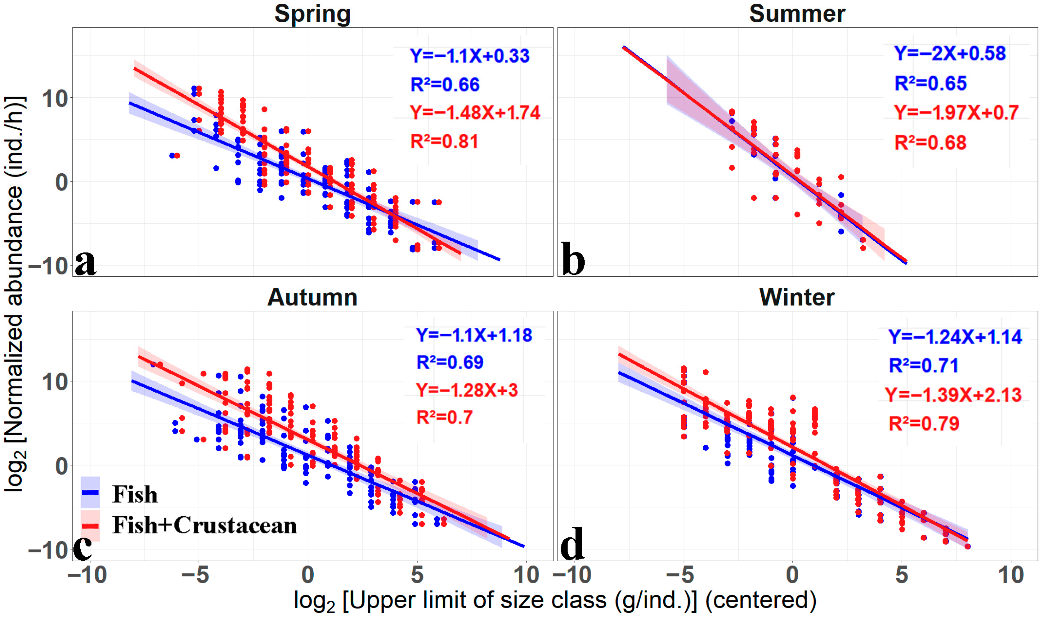
The fish spectra curve with or without crustaceans exhibited a typical declining shape with abundance negatively associating with average body size. The f_slope (fisheries size spectrum slope) value was −1.1, −2, −1.1 and −1.24 for spring, summer, autumn and winter, respectively. The all fitted R2 were higher than 0.65, indicating that the log-linear size spectrum curve was well fitted. The size spectrum curve was steepest in summer, while it was shallower in spring and autumn (Figure 2, Table 1). The slope of adding crustacean (f+c_slope: fisheries+crustacean size spectrum slope) were observed across seasons (Figure 2, Table 1). The slope decreased from −1.1, −1.1 and −1.24 to −1.48 (ΔSlope = −0.38), −1.28 (ΔSlope = −0.18) and −1.39 (ΔSlope = −0.15) in spring, autumn and winter, respectively, while in the summer, it increased from −2 to −1.97 (ΔSlope = +0.03); the adding of crustaceans was significant in all seasons except summer (p < 0.01, t test, d.f. = 40, Figure 2, Table 1).
The significant seasonal difference in the f_slope and f+c_slope was also shown on the boxplot (d = 4, anova p < 0.05), which is caused by the summer lowest slope. However, the boxplot of ΔSlope showed a non-significant seasonal difference (d = 4, anova p > 0.05), indicating the adding effect of crustaceans was different for summer and other seasons, with the positive and negative effect in summer and other seasons, respectively (Figure 3).

3.2.2. Seasonal Variation in Re-Scaled Size Spectrum Intercepts (f_heights) and Abundance

The re-scaled size ranged from 2−6 to 26, 2−3 to 23, 2−7 to 27, and 2−5 to 28, (with original axis size scale corresponding to 2−2 to 210, 23 to 29, 2−2 to 210 and 2−1 to 212) for spring, summer, autumn and winter, respectively (Figure 3). Since the re-scaled size axis (zero-centralized) analysis only changed the intercept, which depends largely on the abundance [16], we compared the distribution of re-scaled heights and its abundance. The slope (f_slope and f+c_slope) and R2 were the same as the original curve, but the intercept decreased accordingly, because the re-scaled zero is always in the center, compared to the original zero in the left part of the curve (Figure 3). The f_ height and f+c_height were 0.33, 0.58, 1.18, 1.14 and 1.74, 0.7, 3, 2.13 in the spring, summer, autumn and winter, respectively (Figure 4a–d, Table 2). The overall f_height (>1) and f+c_height (>2) were both high in autumn and winter, and both low (<1 for f_height, and <2 for f+c_height) in spring and summer. Meanwhile, their difference (∆height) was high in spring and autumn (>1), and low in summer and winter (<1). ∆height was 1.41, 0.12, 1.82 and 0.99 in the spring, summer, autumn and winter, respectively (Table 2). The seasonal variation in log∆abundance was similar to that of ∆height, indicating that the adding crustaceans induced the seasonal change in ∆height (Table 2).

3.2.3. Spatial Distribution of Normalized Size Spectrum Slopes

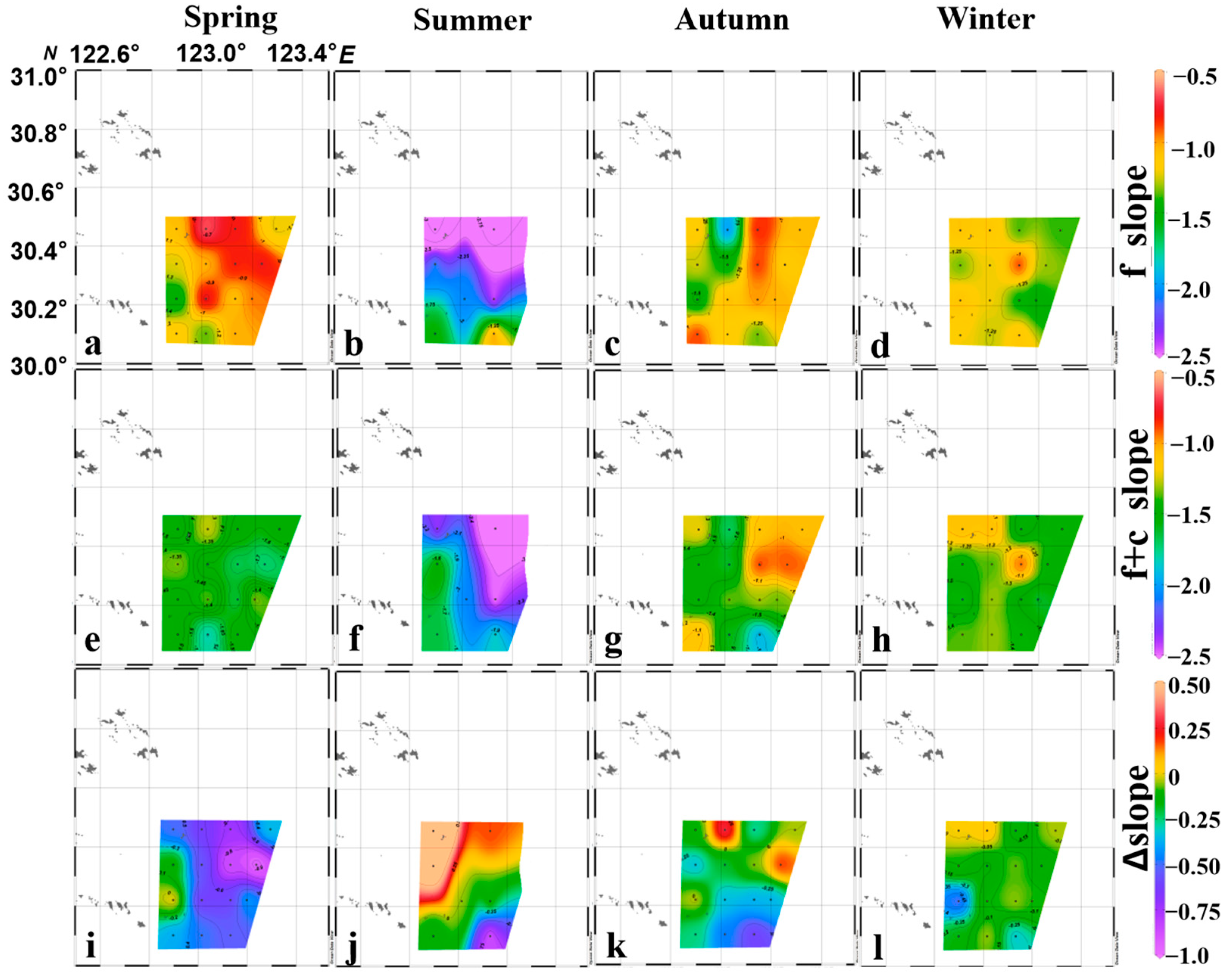
The spatial distribution of f_slope and f+c_slope were heterogeneous in summer and autumn (Figure 5b,c,f,g), while they were more homogeneous in spring and winter (Figure 5a,d,e,h). As described in the above section, f_slope and f+c_slope were deeper in summer, and shallower in other seasons in all the spatial grids (Figure 5a–h). ∆slope indicated the adding effect of crustaceans, and it showed a strong steeping effect in spring and autumn, especially in the offshore of the study regions in the spring (∆slope < −0.5, Figure 5i), and south of the study regions in the autumn (∆slope < −0.5, Figure 5k). The mild steeping effect was found in the majority of southern study regions in the winter (∆slope < −0.25, Figure 5l). Compared to the steeping effect in other seasons, a strong adding (curve becoming shallow) effect was observed in most northern study regions in the summer (∆slope > 0, Figure 5j).

3.3. Spatial Distribution of Re-Scaled Size Spectrum Intercepts (Heights) and Abundance

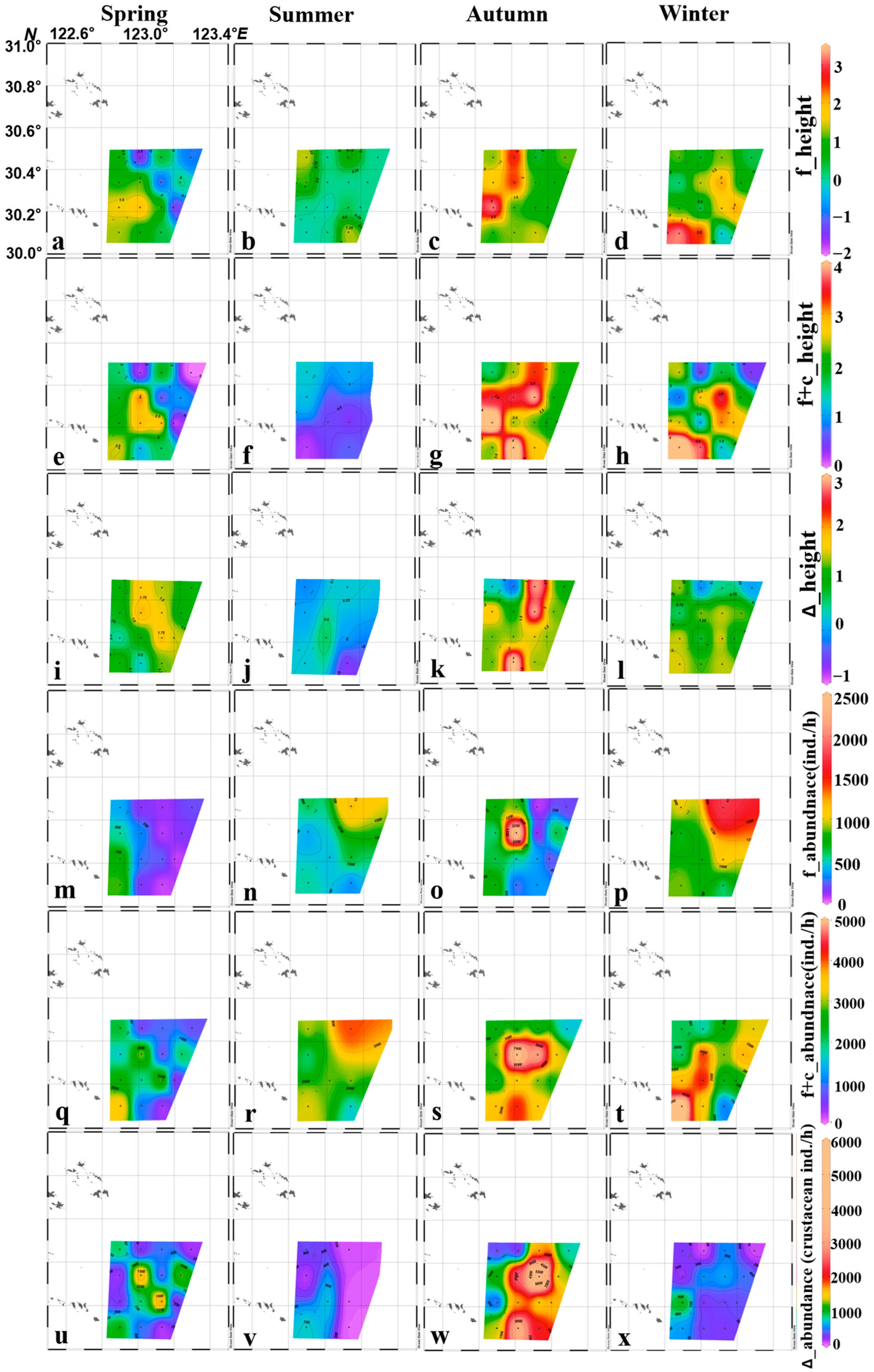
The spatial distribution of f_height and f+c_height showed a strong heterogeneous pattern in autumn and winter when abundance was high, while the distribution was relatively homogeneous in spring and summer with lower abundance (Figure 6a–h). The distribution of f+c_abundance also showed a similar pattern of that for f_height and f+c_height, while the distribution of f_abundance was not consistent with f_height, because of low abundance in autumn (Figure 6m–t). ∆abundance reflected the abundance of only crustaceans, the ∆height indicated the effect of adding crustaceans, the distribution of these two parameters showed consistent patterns in all the seasons. More crustaceans were observed to be added to the whole community in spring and autumn than in summer and winter, especially in the east offshore of the study region. The ∆height and ∆abundance showed more homogeneous distribution in summer and winter, when the crustaceans were few (Figure 6i–l,u–x).
It is also noted that larger numbers of fish species were found in the west side of study region in spring and autumn, as contrary to the high abundance distribution in the east side of the study region in summer and winter (Figure 6m–p). However, after adding the crustaceans, the spatial distribution pattern was reversed in the two seasons(spring and autumn), with west of study region fewer and east more abundance, respectively, vice versa in summer and winter (Figure 6u–x). The comparison of adding crustaceans showed the offset effect of fish and crustaceans in both the temporal and spatial scale.

4. Discussion

4.1. Spatial–Temporal Patterns of Normalized Size Spectrum Slopes of Fisheries Community

The size spectrum of fisheries communities have long been studied in lakes, coastal seas, as well as the open ocean [3,8]. Many studies suggested that the slope of fisheries communities were nearly −2 in the open oceans [16,17], and it was a good indicator to examine the status of fisheries exploitation and climate change [18]. Based on the size spectrum analysis, our study provided good indicators (slope and intercept) to investigate the seasonal variation in fishery communities with or without crustaceans, and found that the f_slope was much more shallower than −2 in spring (−1.1), autumn (−1.1) and winter (−1.24), while it was close to −2 in summer. The shallowest (largest, f_slope = −1.1) slope was found in the spring, which may indicate that the spawning of a number of large size fish and few juveniles during the spring survey was probably the factor causing the slope as evidenced by other studies in the ECS [19,20]. In spring, it was the season of economic fish such as matured fish Lophius litulon, Larimichthys polyactis, Miichthys miiuy, Scomberomorus niphonius, etc., which may migrate to traditional spawning grounds such as our study region [21,22]. Hence, spawning aggregation of the large, matured species in the study region has led to the shallowest slope in spring. Meanwhile, in summer, a great number of small fish organisms had just grown to the capture stage, as well as the few large-sized predators, which may have led to the steepest slope. Indeed, in summer 2022, a giant jellyfish bloom was observed in almost every station in our study region, which probably led to fewer large-body fish due to the porins/cytolysins trigger escaping (unpublished data). Fishing efforts were minimal in summer because of the fishing moratorium; however, large-sized fish were so few that other factors, rather than fishing reduction, may have contributed to the slope variation, as we suggested above. The effect of the fishing moratorium was widespread in the ECS regions due to the strict execution of fishing management in summer as shown by the studies of Li et al. (2005) and [19]. Hence, the jellyfish bloom may have benefit from the fishing moratorium during summer, which resulted in more reduced fishing pressure of jellyfish, rather than fish. This hypothesis may be tested in future investigations. It was also found that smaller fish organisms were the small yellow croaker (Larimichthys polyactis), and the pomfret (Pampus argenteus), which may have contributed to a high abundance of small-bodied species due to their larval stage being in the summer. The f_slope in spring and winter became shallower probably due to the growth of organisms and the migration of some species, which may have been caused by temperature variations [21].
Spatially, the f_slope distribution pattern in the nearshore and offshore side seems to be reversed in the autumn and winter, respectively (Figure 5a–l). However, studies of the distribution of environmental variables (especially temperature and salinity) on the east and west side showed a homogeneous pattern during autumn to winter [21,23]; hence, it is highly speculated that the fishing effort resulted in slope distribution pattern dynamics from autumn to winter. That is, high and low fishing efforts during autumn in the nearshore and offshore, respectively, and such a distribution pattern of fishing effort was reversed in winter. This is probably because fishing vessels were concentrated in coastal regions just after the fishing moratorium, due to the highly available resources in autumn, and they moved outside gradually because of fewer existing resources, but were still high in the offshore regions. We will develop a study to connect our findings with the fishing effort distribution in the near future.

4.2. Seasonal Variation in the Adding Effect of Crustaceans on the Fisheries Communities

Fish and crustaceans are usually separated into different communities, and are assumed to have their own functional traits [4,11]. However, recent studies suggested the considerable overlap existed in resources using them [23]. The inclusion of crustaceans was tested on both the spatial and temporal scale in our study. We found that the adding effect of crustaceans was greater in lower temperature seasons (the spring and winter bottom temperature was 14.4 °C and 14.5 °C; see the study of Zhang et al., 2025 [12]; the steepening effect was around −0.4 and −0.7 for spring and winter, respectively), and the adding effect was small in the relatively warmer seasons (summer and autumn bottom temperature was 22.3 and 22.5 °C). Heather et al. (2021) examined the inclusion of invertebrates with fisheries communities at the global scale [8], and suggested the inclusion effect was greater in temperate waters (such as polar areas), and small in the tropical areas. Our study, based on the seasonal datasets, partially supported the conclusion, with few crustaceans in summer, and more abundant crustaceans in spring and autumn. It was found that one mantis shrimp (Oratosquilla oratoria) and three crab species (Charybdis japonica, Portunustri tuberculatus, and Charybdis bimaculata) were dominant in the spring and autumn season, and they contributed greatly to the adding effect in these two seasons. It seems that fish and crustacean species were mismatched with each other in spatial (offshore–nearshore) and temporal (temperate season–warm season) scales. It was assumed that the spawning and reproductive behavior of the two species induced the difference. Fish species generally aggregated to spawn in the spring, while crustaceans spawned in the summer, whereas both species reached a large size with few numbers, in these two seasons, respectively [12]. However, there are still uncertainties when it comes to the spawning flexibility of individual species, such as Trichiurus lepturus (hairtail), which exhibited multiple spawning seasons due to climate change. We will explore the effect of these uncertainties (multiple spawning species) on the seasonal variation in f_slopes in the future. Generally, the adding of crustaceans induced a higher R2 of regression fitting in all seasons (Table 2), indicating the interaction of fish and crustaceans existed in the whole ecosystem, as other studies suggested [18]. Their food resource-sharing and prey–predator relationship are probably the key aspects we should examine in the next step.
To sum up, based on a size spectrum analysis, our study provided a case study to resolve the seasonal variation in fish and fish-plus-crustaceans community parameters (slope and intercept). The results showed that crustaceans are the main components of fisheries ecosystems in the ECS. Size spectrum analysis with or without the crustaceans in the fisheries communities cannot reveal the trophic interaction, which may be studied further. Moreover, the driving factors of spatial and temporal variation in slopes are the key issues for fisheries management, which were not covered by our current study, and should be considered in the future.

Author Contributions

All authors contributed to the design of the study, data collection, analysis and writing of this manuscript. All authors have read and agreed to the published version of the manuscript.

Funding

This work was supported by the National Key R&D Program (2023YFD2401904; 2024YFD2400703) of Ministry of Science and Technology, China and the Fisheries Resource Dynamic Monitoring and Survey Project in Zhejiang Fishing Grounds (HYS-CZ-202405) of Zhejiang Province, China.

Data Availability Statement

Data available on reasonable request.

Conflicts of Interest

The authors declare no conflicts of interest.

References

  1. Zhang, H.; Song, P.; Li, Y.; Liu, S.; Wang, X.; Zheng, J.; Lin, L. Diversity and Community Structure of Nekton in the South-Central East China Sea in Autumn. J. Appl. Oceanogr. 2021, 40, 575–586. (In Chinese) [Google Scholar]
  2. Blanchard, J.; Heneghan, R.; Everett, J.; Trebilco, R.; Richardson, A.J. From bacteria to whales: Using functional size spectra to model marine ecosystems. Trends Ecol. Evol. 2017, 32, 174–186. [Google Scholar] [CrossRef]
  3. Marshall, A.; Bigg, G.; Leeuwen, S.M.; Pinnegar, J.K.; Wei, H.; Webb, T.J.; Blanchard, J.L. Quantifying heterogeneous responses of fish community size structure using novel combined statistical techniques. Glob. Change Biol. 2016, 22, 1755–1768. [Google Scholar] [CrossRef]
  4. Blanchard, J.; Andersen, K.; Scott, F.; Hintzen, N.T.; Piet, G.; Jennings, S. Evaluating targets trade-offs among fisheries conservation objectives using a multispecies size spectrum model. J. Appl. Ecol. 2014, 51, 612–622. [Google Scholar] [CrossRef]
  5. Barneche, D.; Kulbicki, M.; Floeter, S.; Friedlander, A.M.; Maina, J.; Allen, A.P. Scaling metabolism from individuals to reef-fish communities at broad spatial scales. Ecol. Lett. 2014, 17, 1067–1076. [Google Scholar] [CrossRef] [PubMed]
  6. Heather, F.; Stuart-Smith, R.; Blanchard, J.; Fraser, K.; Edgar, G. Reef communities show predictable undulations in linear abundance size spectra from copepods to sharks. Ecol. Lett. 2021, 24, 2146–2154. [Google Scholar] [CrossRef] [PubMed]
  7. Jennings, S. Indicators to support an ecosystem approach to fisheries. Fish Fish. 2005, 6, 212–232. [Google Scholar] [CrossRef]
  8. Heather, F.; Blanchard, J.; Edgar, G.J.; Trebilco, R.; Stuart-Smith, R.D. Globally consistent reef size spectra integrating fishes and invertebrates. Ecol. Lett. 2021, 24, 572–579. [Google Scholar] [CrossRef]
  9. GB/T 12763.6-2007; Specifications for Oceanographic Survey—Part 6: Marine Biological Survey. Standardization Administration of China: Beijing, China, 2007.
  10. SC/T 9403-2012; Technical Specification for Marine Fishery Resources Survey. Ministry of Agriculture and Rural Affairs of the People’s Republic of China: Beijing, China, 2012.
  11. Yu, C.; Song, H.; Yao, G. Study on the Community Structure Characteristics of Crabs in the East China Sea. Oceanol. Limnol. Sin. 2005, 36, 213–220. (In Chinese) [Google Scholar]
  12. Zhang, Z.; Xu, Y.; Zhang, X.; Chen, F.; Zhou, Y.; Xu, K.; Zhang, Y.; Zhang, H.; Li, Q.; Liu, W.; et al. Seasonal changes of community structure of fish and crustaceans in the adjacent waters of Shengsi Ma’an Islands. J. Fish. China 2025, 49, 059308. [Google Scholar]
  13. Wilson, S.; Fisher, R.; Pratchett, M.S.; Graham, N.A.J.; Dulvy, N.K.; Turner, R.A.; Cakacaka, A.; Polunin, N.V.C. Habitat degradation and fishing effects on the size structure of coral reef fish communities. Ecol. Appl. 2010, 20, 442–451. [Google Scholar] [CrossRef]
  14. Daan, N.; Gislason, H.; Pope, J.; Rice, J.C. Changes in the North Sea fish community: Evidence of indirect effects of fishing? ICES J. Mar. Sci. 2005, 62, e177–e188. [Google Scholar] [CrossRef]
  15. Guo, J.; Chen, Z.; Xu, S. Research Progress on Fish Size Spectrum. Mar. Fish. 2017, 39, 582–591. (In Chinese) [Google Scholar]
  16. Jennings, S.; Mackinson, S. Abundance-body mass relationships in size-structured food webs. Ecol. Lett. 2003, 6, 971–974. [Google Scholar] [CrossRef]
  17. Carsten, R. The role of spatial scale and the perception of large-scale species-richness patterns: Scale and species-richness patterns. Ecol. Lett. 2004, 8, 224–239. [Google Scholar] [CrossRef]
  18. Trebilco, R.; Baum, J.; Salomon, A.; Dulvy, N. Ecosystem ecology: Size-based constraints on the pyramids of life. Trends Ecol. Evol. 2013, 28, 423–431. [Google Scholar] [CrossRef] [PubMed]
  19. Li, S.; Cheng, J.; Li, C.; Li, J. Seasonal Variation in Fish Community Diversity in the Central East China Sea. Mar. Fish. 2005, 27, 113–119. (In Chinese) [Google Scholar]
  20. Xu, Y.; Jiang, R.; Hao, Q.; Zhu, W.; Szuwalski, C.; Wang, S.; Yu, C. Effects of environmental change and exploitation on marine communities around the Zhoushan archipelago: A functional group perspective. Estuar. Coast. Shelf Sci. 2019, 217, 185–195. [Google Scholar] [CrossRef]
  21. Xu, Y.; Yu, C.; Zhang, P.; Deng, X.; Zhang, Z.; Shen, H. Community Structure of Springtime Nekton and Its Relationship with Environmental Factors in the Hangzhou Bay-Zhoushan Offshore Area. J. Fish. China 2019, 43, 605–617. (In Chinese) [Google Scholar]
  22. Yan, L.; Liu, Z.; Li, S.; Ling, J.; Li, J.; Li, Z. Effects of new summer close season of trawl fisheries on fishery ecology and resource enhancement in East China Sea. Mar. Fish. 2010, 32, 186–189. (In Chinese) [Google Scholar]
  23. Donovan, M.; Friedlander, A.M.; Lecky, J.; Jouffray, J.-B.; Williams, G.J.; Wedding, L.M.; Crowder, L.B.; Erickson, A.L.; Graham, N.A.J.; Gove, J.M.; et al. Combining fish and benthic communities into multiple regimes reveals complex reef dynamics. Sci. Rep. 2018, 8, 16943. [Google Scholar] [CrossRef] [PubMed]
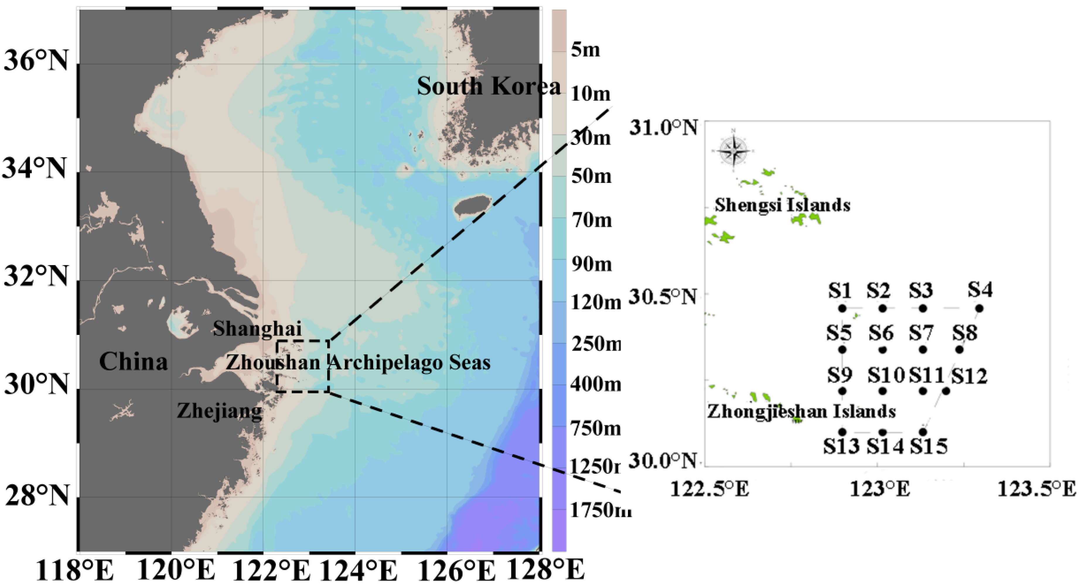
Figure 1. Distribution of survey stations.
Diversity 17 00744 g001
Figure 2. The seasonal variation in normalized abundance size spectrum of fish with (red curve) or without (blue curve) crustaceans by log-linear regressions. Note: the regression parameters (slope, intercept and R2) were shown in the top right of each figure in spring (a), summer (b), autumn (c) and winter (d).
Diversity 17 00744 g002
Figure 3. Boxplot of seasonal differences in the f_slope and f+c_slope and its difference. Note: the regression parameters (slope, intercept and R2) were obtained from equations in Figure 2.
Diversity 17 00744 g003
Figure 4. The seasonal variation in re-scaled × axis size spectrum parameters of fish with (red curve) or without (blue curve) crustaceans by log-linear regressions. Note: the re-scaled f_slope was the same as the original f_slope, re-scaled f_intercept was replaced by f_height to differ from the original f_intercept. The fitted curves and regression functions were also shown in the figure, respectively. (ad) indicates fitted parameters in spring, summer, autumn and winter, respectively.
Diversity 17 00744 g004
Figure 5. The spatiotemporal distribution of the f_slope, f+c_slope and ∆slope in spring, summer, autumn and winter. Note: f_slope, f+c_slope and ∆slope represent the slopes of normalized abundance size spectrum for “fish” and “fish+crustaceans” and its difference, respectively; (ad) are f_slopes, (eh) are f+c_slopes, and (il) are ∆slopes for four seasons, respectively.
Diversity 17 00744 g005
Figure 6. Spatial distribution of re-scaled fish only community size spectrum intercepts (f_height, (ad)), fish plus crustacean community size spectrum intercepts (f+c_height, (eh)), difference in f+c_height and f_height (∆_height, (il)), fish abundance (f_abundance, (mp)), fish plus crustacean abundance (f+c_abundance, (qt)) and Δ_abundance of its difference (crustaceans) in four seasons (ux).
Diversity 17 00744 g006
Table 1. IRI of dominant fish and crustacean species in the whole year (with IRI ≥ 100 showing common species, * indicating dominant species, IRI > 1000).
CommunityOrderFamilySpeciesIRI in SpringIRI in
Summer
IRI in
Autumn
IRI in
Winter
FishSynodontidaeAulopiformesHarpadon nehereus991.33215.801415.28 *11,797.04 *
AcanthuriformesSciaenidaeJohnius belangerii2840.51 *-182.79-
LophiiformesLophiidaeLophiomus setigerus2338.41 *--289.47
AcanthuriformesSciaenidaeLarimichthys polyactis-2949.72 *--
ScombriformesTrichiuridaeTrichiurus japonicus207.232258.21 *--
PerciformesTriglidaeChelidonichthys kumu256.141073.84 *-561.04
CarangiformesCarangidaeTrachurus japonicus-4759.19 *--
MyctophiformesMyctophidaeBenthosema pterotum---1281.26 *
CrustaceansStomatopodaSquillidaeOratosquilla oratoria2855.68 *-697.071168.53 *
DecapodaPortunidaeCharybdis japonica504.39-1875.96 *227.58
DecapodaPortunidaePortunus trituberculatus796.41309.362351.32 *142.76
DecapodaPortunidaeCharybdis bimaculata1284.57 *1419.02 *4384.87 *321.78
Table 2. Seasonal variation in f_slope, f+c_slope, re-scaled intercept, R2 and abundance.
Season Fish Fish+Crustacean
f_Slope f_intercept Re-scaled
f_intercept
(f_height)
Log (Fish Abundance) R2 f+c_Slope f+c_interceptRe-scaled
f+c_intercept
(f+c_height)
∆HeightLog(fish+
Crustaceans Abundance
∆log
(Abundance)
R2
Spring−1.14.950.335.64 0.66−1.487.621.741.416.82 1.18 0.81
Summer−212.140.586.88 0.65−1.9712.080.70.127.13 0.25 0.68
Autumn−1.15.671.186.38 0.69−1.287.8231.827.74 1.36 0.7
Winter−1.246.081.147.17 0.71−1.397.662.130.997.42 0.25 0.79
Disclaimer/Publisher’s Note: The statements, opinions and data contained in all publications are solely those of the individual author(s) and contributor(s) and not of MDPI and/or the editor(s). MDPI and/or the editor(s) disclaim responsibility for any injury to people or property resulting from any ideas, methods, instructions or products referred to in the content.