Pluridecadal Temporal Patterns of Tintinnids (Ciliophora, Spirotrichea) in Terra Nova Bay (Ross Sea, Antarctica)

Abstract

During the next century, the Ross Sea is expected to reduce summer sea ice concentrations and consolidate the presence of shallower mixed layers. Those changes may have a potentially catastrophic effect on the zooplankton community. To investigate if Ross Sea’s past physical and biological condition changes have affected the tintinnids population, and to understand future tintinnids’ role in the plankton community, seawater samples collected in the Terra Nova Bay polynya area during eleven summer expeditions from 1988 to 2017 were analyzed. During this time period, tintinnids’ abundance ranged from 0 to a maximum of 4980 indL⁻¹. The most representative species were Cymatocylis drygalskii, Codonellopsis gaussi and Laackmanniella naviculifaera. These species can be considered keystone species and they can be used to monitor the long-term evolution of the whole microzooplankton community in Terra Nova Bay polynya. The tintinnids’ abundance presented minimum values in 2001 after which there has been a significant increase in the most recent years. The increase in tintinnids’ abundance showed a positive correlation with the temperature, while salinity did not indicate any relationship. In particular, the majority of genera detected showed a significant temperature correlation, with the only exception of Amphorides genus, recorded for the first time in the study area. Our results provide new insights into the spatial distribution and structure of the Antarctic tintinnids community.

1. Introduction

On decadal time scales, the Ross Sea has been experiencing changes in both its physical and biological conditions. In the last 60 years, the Ross Sea shelf waters have undergone a continuing near-linear temperature increase and salinity decrease [1], although a rebound in salinity was observed from 2016 to 2019 [2,3]. Similar interannual variability has been observed in sea ice concentration that has increased from 1979 to 2014 [4] and decreased during the summer after 2015 [3].

Thermohaline changes are most evident in Terra Nova Bay (TNB) which is located in the western sector of the Ross Sea off Victoria Land and is bounded by the Drygalski Ice Tongue to the south and the Campbell Ice Tongue to the north. Here, the salinity of the Dense Shelf Water (DSW) decreased from 1995 to 2014 by −0.045 ± 0.016 dec⁻¹, with a change in neutral density from 28.796 to 28.718 kg m⁻³ [2]. After 2014, a sharp increase in salinity has been observed with a rebound to values last observed in the mid-late 1990s [2]. Superimposed on this trend, Castagno et al. [2] also observed an interannual variability with 5–10 years fluctuations. Relative minimum values were registered in 2000, 2005, and 2014, whereas relative maximum values were measured in 1995, 2002, 2008, and 2018 [2,3]. These salinity anomalies extend throughout the water column [2], with the surface water showing the same variability as the DSW, (see Figure 3a in Castagno et al. [2]). DSW temperatures have increased in proportion to the rise in sea surface freezing point that would accompany the observed salinity decrease [5].

The predominant feature of TNB is a coastal latent heat polynya formed and maintained by katabatic winds [6]. TNB polynya is bounded by the Drygalski Ice Tongue to the south that acts as a barrier for the pack ice advection from the south [7], keeping the polynya open during winter. The mean polynya extent during winter ranges from 1000 to 1300 km² estimated from thermal infrared data [6,7] to about 4200 km² using passive microwave data [8]. However, the polynya extent shows a large interannual variability [9]. TNB polynya influences the entire water column, the persistent sea-ice production, and export by the katabatic winds during winter results in brine rejection that densifies the water column. TNB water column could be divided into an upper layer of about 150 m characterized by high thermohaline variability and a layer beneath where the water column is nearly isothermal, and the vertical stability is preserved by the increasing salinity [9]. During winter, from May to October, surface water temperature is close to the freezing point, while salinity increases due to brine rejection in response to sea ice formation [9]. Starting from November, temperature increases, and salinity decrease due to sea ice melting and the heat gained from the solar radiation [10]. Due to a large amount of sea ice melting associated with increased springtime temperatures the TNB water column becomes highly stratified in late spring and summer [11]. Furthermore, in early austral spring, TNB polynya greatly increases in size [12], and hosts large seasonal phytoplankton blooms, typically dominated by the colonial haptophyte Phaeocystis antarctica in spring through early summer, with an increase in abundance of diatoms in mid to late summer [11,12,13,14,15,16]. The summer diatom blooms are documented by a European Long Term Ecological Research (LTER) data, initiated in 2006 near the Italian station Mario Zucchelli in TNB (http://www.lteritalia.it/?q=macrositi/it17-stazioni-di-ricerca-antartide accessed on 21 July 2022) as well as by previous expedition to TNB (from 1987 to 1995) [17].

Recent studies suggest that future phytoplankton assemblage and productivity will likely increase due to changes in summer sea ice concentrations and hypothesize that shallower mixed layer depths will cause diatoms to dominate the future phytoplankton assemblage relative to P. antarctica [18,19,20]. The considerable increases in phytoplankton biomass and large size structure suggest that the Ross Sea could now be extremely productive in summer [20] and these changes in phytoplankton composition, productivity, and export would have implications for the rest of the Ross Sea food web as provide increased energy to grazers and thus increase secondary production.

Microzooplankton organisms (20 µm to 200 µm size range) are pivotal species in the microbial community and they play a fundamental role in the Antarctic food webs [21,22]. Microzooplankton herbivory constitutes a major source of mortality for phytoplankton in the ocean [23,24,25] and may thus exert significant top-down control on phytoplankton blooms in the Southern Ocean [21,22].

Tintinnid ciliates are part of microzooplankton, which in the Southern Ocean sometimes represent up to 50% of microzooplankton abundance and biomass [26]. They are characterized by a species-specific shell (lorica), shaped like a bowl or vase, or tube [27] on which their taxonomy is based. Some tintinnids species are known to display considerable plasticity in lorica morphology, (e.g., [28,29,30]), which has led to a different classification of some species over the years.

In the Southern Ocean, tintinnids appear to be a widely important and exploited food resource. They are feeding primarily on small phytoplankton sizes and, when phytoplankton is not dominated by large diatoms or Phaeocystis, they are recognized to be the major consumers of primary production. Moreover, a wide variety of animals are known to consume tintinnids. They have been found in the guts of crustacean zooplankters such as copepods [31], krill and mysid shrimp [32], salps [33], chaetognaths [34], and larval Antarctic silverfish [35].

The Antarctic waters’ studies on tintinnids date back to the earliest scientific expedition and they were almost exclusively devoted to taxonomic description [36,37]. The most recent reports provide quali-quantitative data and they are available for different Antarctic environments [38,39,40,41,42,43]. Despite the relatively abundant data on tintinnids distribution and composition, to the best of our knowledge, there are no long time series on tintinnids in the Antarctic area.

In this paper, we report the first plurennial series on tintinnids collected on eleven occasions in the polynya of TNB over the period 1988–2017. The aim of this study was to describe the tintinnids community in TNB over the past thirty years and analyze if tintinnids were affected by the significant changes in the Ross Sea environment. We hypothesize that the rising ocean temperature, as expected from climate change predictions, might have an effect on tintinnids’ community structure, with ecological consequences in its quantity and diversity, including modification of keystone species.

2. Material and Methods

Tintinnids’ community was studied during eleven expeditions in the Ross Sea within the frame of the Italian Project in Antarctica (PNRA) in the Terra Nova Bay (TNB) polynya (74°60–75°40 S and 163°50–167° E), between the Campbell Glacier Tongue and Drygalskii Ice Tongue (Figure 1). Sampling was performed during the austral summer (December–February) of each expedition.

Table S1 reports the sampling site and number of stations for each year. Samples were collected using 12 L Niskin bottles (Sea-Bird Electronics 32) mounted on a multisampler equipped with a CTD sensor (Meerestechnik Mod. KMS multiparametric; 9/11 Plus, Sea-Bird Electronics, Bellevue, WA, USA). Sea water samples were collected at 3 to 5 depths, relative to the surface, DCM (deep chlorophyll maximum), and intermediate depths depending on the bottom of the sampled site (max sampled depth 1128 m). In total, 321 seawater samples were analyzed. Temperature and salinity values used in the following analyses correspond to the depths where Niskin bottle samples were taken for tintinnids samples.

During the expedition of January–February 1990, we sampled repeatedly at two coastal stations: MER (Mergellina) with a bottom depth of 25 m and SMN (Santa Maria Novella) with 500 m depth. In 1994, only one station was considered in this paper, as the long transect sampled was outside of the Terra Nova polynya. In 2011/12 we sampled repeatedly at six stations: SMN, PTF (Portofino), FAR (Faraglioni), T10, and TER (Tergeste), the last two closers to Mario Zucchelli Station (MZS) (Table S1).

At each depth, from 2 to 5 L of seawater was reverse-filtered through a 10 µm mesh, in order to reduce the volume to 250 mL and immediately fixed with buffered formaldehyde (1.6% final concentration). Subsamples (50 mL) were then examined in a settling chamber using an inverted microscope (magnification 200×) (Leitz Labovert, Leica DMI 300B, Wetzlar, Germany), according to the Utermöhl method [44]. The entire surface of the chamber was examined.

Tintinnids encountered were assigned species names based only on lorica morphology. Many species in the Antarctic are considered morphological variants [29,30] and molecular analyses could be useful to distinguish between different species. In this study, the samples were fixed with formalin and the tintinnids species identifications were made on the basis of description by Brand [45,46], Laackmann [36,37], Kofoid and Campbell [47,48], Alder [49], and Petz [50].

Empty loricae were not differentiated from filled ones because tintinnid protoplasms are attached to the lorica by a fragile strand, which detaches with ease during collection and fixation of the samples.

Salpingella genus showed considerable variability in lorica length that made the identification extremely difficult and uncertain. For this reason, we did not distinguish the different Salpingella species and for the calculation of the biomass we divided this genus into different classes according to the different lengths (from 70 to 200 µm). The oral diameter varied from 15 to 20 µm.

For each species, the biomass was estimated by measuring the linear dimensions of each organism using an eyepiece scale and relating the individual shapes to standard geometric figures. Cell volumes were converted to carbon values using the formula: pgC cell⁻¹ = µm³ × 0.053 + 444.5 [51].

Correlation between biotic and abiotic factors was analyzed using STATISTICA11, StatSoft, TIBCO software, Paloalto, CA, USA and the Spearman correlation index was used to identify the relations between temperature, salinity, and abundance. To test the community composition and the similarity pattern presented by all tintinnids genera, the samples were analyzed on the base of the different depths, years, and coastal distances. The factor “zone” was also considered to divide samples collected in the photic zone (<200 m) from the ones collected in the aphotic one (≥200 m). Multivariate analyses were based on Bray–Curtis similarities index [52], as calculated from the Log (× + 1). PERMANOVA analysis was carried out to test the effect of the considered variable on the community structure. PCO ordination, nMDS, cluster analysis, SIMPER, and ANOSIM analysis were useful to detect which genera were more involved in the communities’ similarity pattern. The analyses were conducted using the PRIMER v7 software, Plumouth, UK [53], and the significance level for all statistical tests was set at 5%.

3. Results

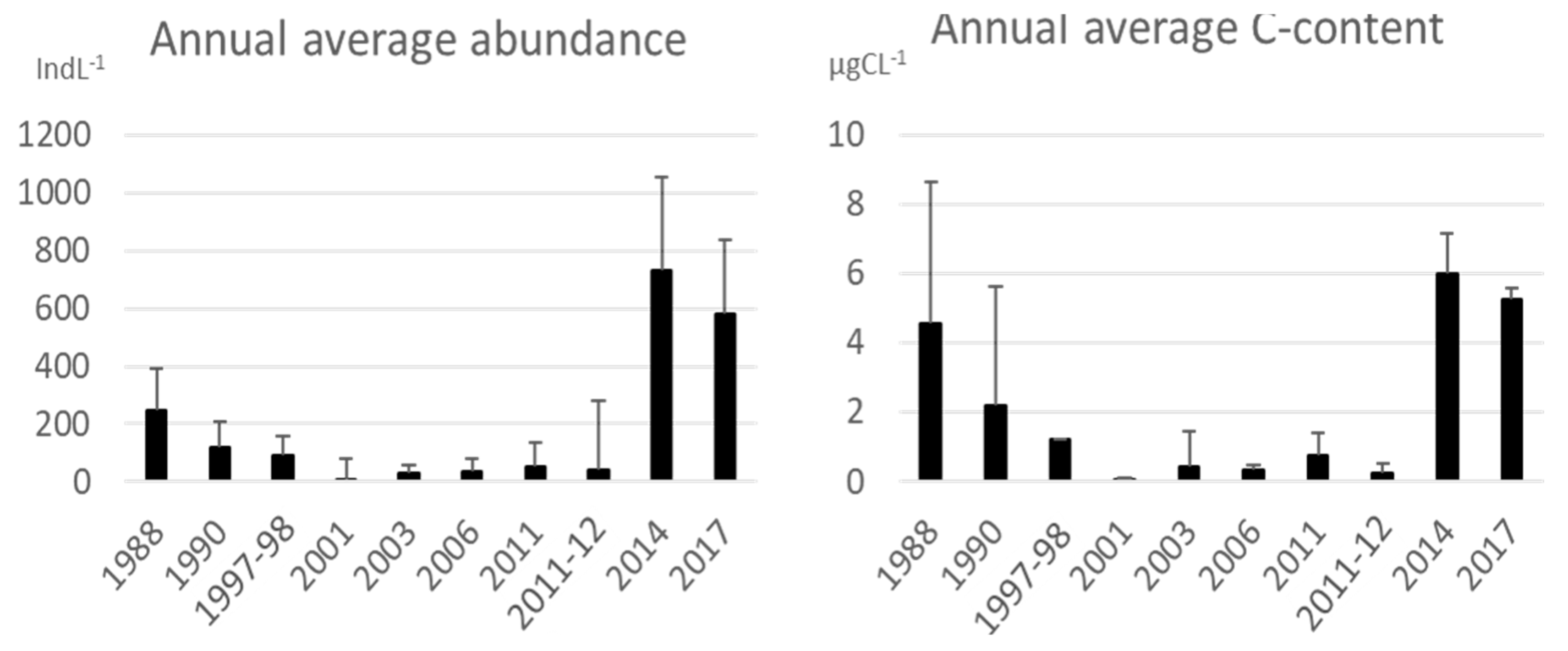
3.1. Tintinnid Abundance and Biomass

The results of multivariate analyses, performed on the entire dataset, point out a significant (PERMANOVA p < 0.05) effect of the factor season (early: December, late: January and February) and the factor layer (photic: <200 m; apothic: ≥200 m), in shaping the community composition. Concerning seasonality, pair-wise test and ANOSIM outputs detected significant (p < 0.05) differences between the communities of the two groups: diversity was mainly due to the higher average abundance and carbon content of the considered taxa. During early summer, the average abundance and the carbon content of all taxa were two orders less than those measured during the late summer (Figure 2).

The maximum abundance detected during the early summer (December 2011) was 14 indL⁻¹ at St. Tergeste (TER) while during late summer (January 2014) the maximum value was 4980 indL⁻¹ at St. 39 (Table S2). As well the carbon content presented higher values in the late summer, with a maximum value of 36 µgCL⁻¹ (St. 39 January 2014).

Considering all the periods and the entire study area, the abundances were higher in the photic zone (<200 m), showing the average abundance of 192 ± 454 indL⁻¹ while in the aphotic zone (≥200 m) they showed a lower value of 10 ± 30 indL⁻¹ (Figure 3). The same trend was detected for the carbon content attesting at the average value of 2.1 ± 3.3 µgCL⁻¹ in the photic zone.

All the genera considered in this work showed the minimum average abundance in the aphotic zone. Pair-wise test and ANOSIM outputs detected a significant (p < 0.05) difference between the communities detected in the two zones highlighting how the aphotic layers (d ≥ 200 m) showed the lowest value in similarity because of the scarce abundances. In order to reduce the variability in the study and to detect the long-term changes in the tintinnids community, only the samples collected in the photic layer (d < 200 m) were considered in the analysis of the genera composition.

The abundance distribution in the upper 200 m of the water column showed a similar average abundance between the surface layer and the intermediate one (10 < d ≤ 100 m) with values of 267 ± 642 indL⁻¹ and 287 ± 384 indL⁻¹, respectively (Figure 4).

The maximum abundance peak was recorded at surface with 4980 indL⁻¹. The maximum abundance at the intermediate depth was 1566 indL⁻¹, while at the 100 < d < 200 m layer the average abundances sharply decreased (MAX = 854 indL⁻¹) at 46 ± 115 indL⁻¹.

The carbon content showed the highest average value at the 10 < d ≤ 100 m layer (3.5 ± 4.1 µgCL⁻¹) thanks to the presence of the genera Cymatocylis and Laackmnniella.

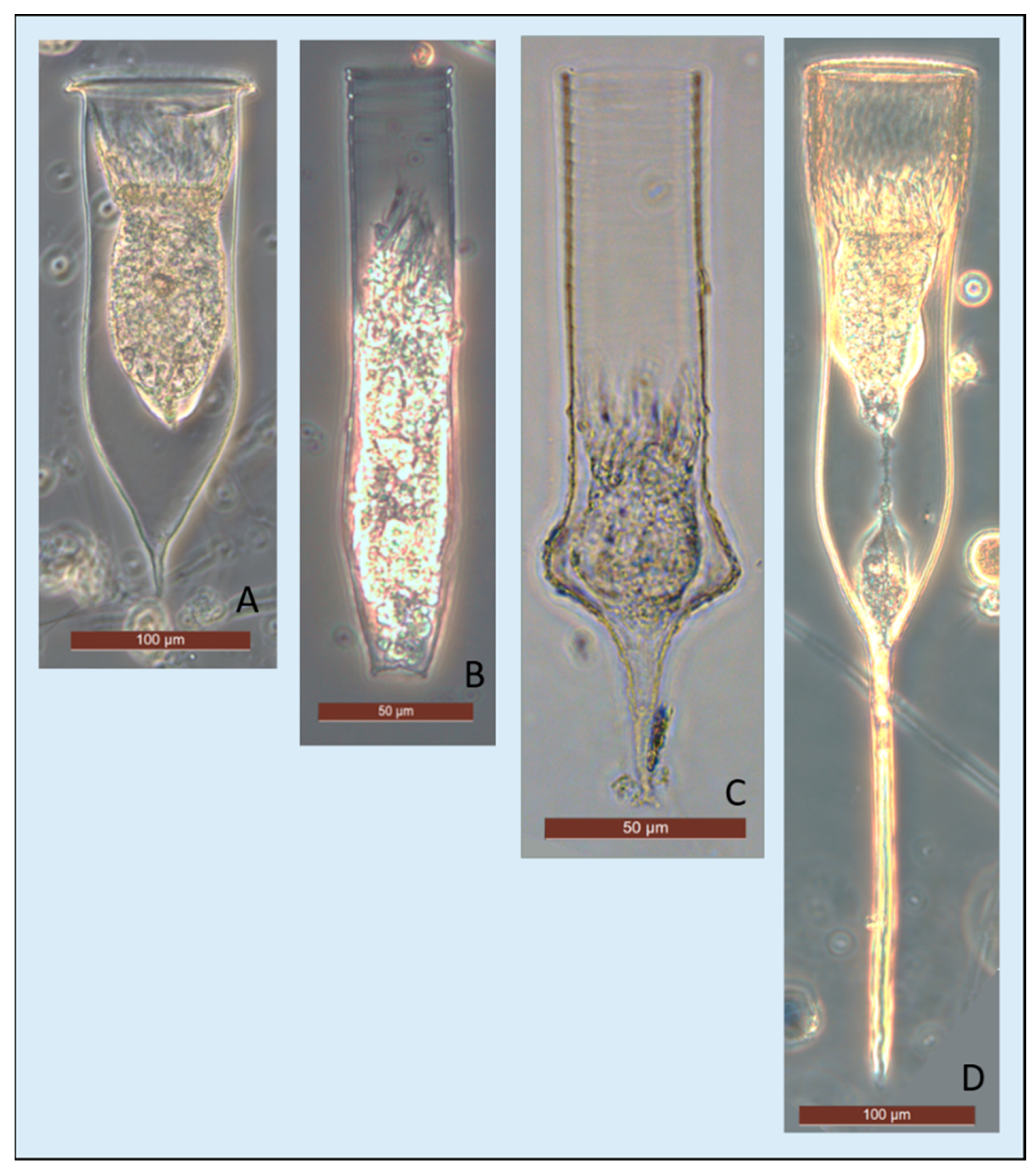
3.2. Tintinnids Composition

In total, 13 taxa, corresponding to 9 species from 5 genera, were identified (

Table 1. List of tintinnid species, ranges of total lorica length, and lorica oral diameter (LOD).

Species	Total Length (µm)	LOD (µm)
Amphorides laackmanni (Jörgensen) Strand, 1928	50–70	15–20
Cymatocylis convallaria Laackmann, 1910	110–140	80–100
Cymatocylis cristallina Laackmann, 1909	180–200	60–80
Cymatocylis drygalskii (Laackmann) Laackmann, 1907	180–340	80–100
Cymatocylis nobilis (Laackmann) Laackmann, 1910	180–200	60–80
Cymatocylis vanhoeffeni (Laackmann) Laackmann, 1910	300–550	80–100
Cymatocylis spp.	110–350	60–100
Codonellopsis gaussi (Laackmann, 1907) Kofoid and Campbell, 1929	125–200	30–35
Codonellopsis glacialis (Laackmann, 1907) Kofoid and Campbell, 1929	80–105	30–40
Codonellopsis spp.	80–200	25–40
Laackmanniella naviculaefera (Laackmann, 1907) Kofoid and Campbell, 1929	125–250	40–50
Laackmanniella spp.	125–250	40–50
Salpingella spp.	70–200	15–20

).

The most representative species were C. drygalskii (Figure 5A), L. naviculaefera (Figure 5B), and C. gaussi (Figure 5C). These three species constituted more than 56% of the tintinnids and they were present in all the years, except in 1994 (sampled only one station) and, for C. gaussi, also in 2012 (

Table 2. List of tintinnid species recorded during the considered period (1988–2017) along the whole water column. (*) species presence.

	1988	1990	1994	1997–1998		2001	2003	2006	2011	2011–2012		2014	2017
Amphorides laackmanni												*	*
Cymatocylis convallaria				*		*		*	*		*
Cymatocylis cristallina		*							*
Cymatocylis drygalskii	*	*			*	*	*	*	*	*	*	*	*
Cymatocylis nobilis		*
Cymatocylis vanhoeffeni	*				*				*			*	*
Cymatocylis spp.	*	*	*	*	*			*	*
Codonellopsis gaussi	*	*		*	*	*	*	*	*	*		*	*
Codonellopsis glacialis	*				*	*			*			*
Codonellopsis spp.	*							*
Laackmanniella naviculaefera	*	*		*	*	*	*	*	*	*	*	*	*
Laackmanniella spp.	*	*						*
Salpingella spp.	*	*	*	*	*	*	*	*	*		*	*	*

). In the last two periods (2014 and 2017), C. drygalskii, L. naviculaefera, C. gaussi and Salpingella genus increased and reached high abundances. In particular, in 2014 Salpingella contributed together with C. drygalskii and C. gaussi, to the highest abundance (4980 indL⁻¹) of all the investigated periods. In this contest, Salpingella showed the value of 3250 indL⁻¹, the highest ever recorded in this time series.

Among the Cymatocylis genus, C. drygalskii was the most common species. It reached a maximum of 1100 indL⁻¹ in 2014 (St. 39, 0 m). Cymatocylis drygalskii presented a wall hyaline cylindrical shape with different lengths of the lorica (180–340 µm), mainly due to the antapical horn (5–100 µm). The collar rim was serrated and bent downwards, and the external diameter of the bowl was quite constant (around 90 µm) and poorly correlated with lorica length. Among the Cymatocylis genus, C. vanhöffeni (Figure 5D) was the second well-represented species, detected with a maximum abundance of 154 indL⁻¹ in 1988 (St. 22, 100 m), especially below 50 m. The bowl elongated hyaline lorica shows an apical region of lorica striated. The size varied from around 400 µm long and 90 µm wide, with a long antapical horn (94–230 µm). The rim was serrated without an outer collar and external opening diameter. Cymatocylis convallaria, C. cristallina, and C. nobilis were very rare, normally detected in the upper 50 m and with maxima abundance < 15 indL⁻¹.

Among the genus Codenollepsis, C. gaussi was the most abundant species with a maximum of 1003 indL⁻¹ in 1988 (St. 32, 0 m). This species presented a short lorica around 130 µm long and 40 µm wide. Codonellopsis glacialis, was not present in all the years and reached the maximum abundance (81 indL⁻¹) in 1997 (St. 214, 0 m). This species presented a size range of around 95 µm in length and 25 µm in width, slightly agglutinated lorica with a bullet-shaped and hyaline annulated short collar that corresponds to the width.

Laackmanniella naviculaefera, with a maximum abundance of 535 indL⁻¹ in 1988 (St. 26, 50 m), presented a cylindrical annulated hyaline lorica sizing around 200 µm long and a very constant opening diameter (around 45 µm).

Amphorides laackmanni was detected only during the last two campaigns (2014 and 2017) with maxima values of 133 indL⁻¹ (St. 15b, 25 m). Amphorides laackmanni presented a hyaline wall with few longitudinal fins, very short body sizing around 60 µm long and 20 µm opening diameter. This species, like the genus Salpingella, is not as peculiar to Antarctic waters.

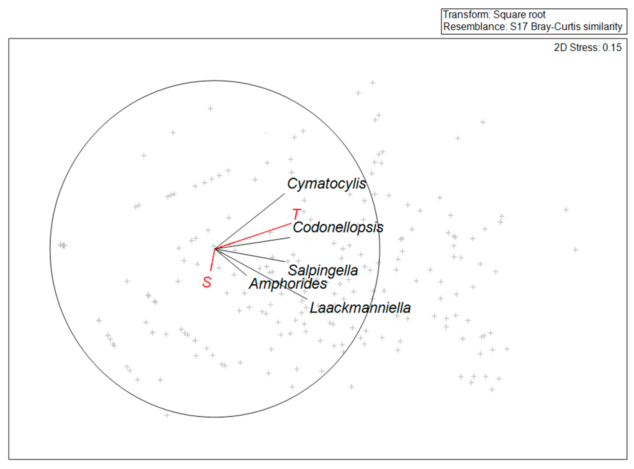
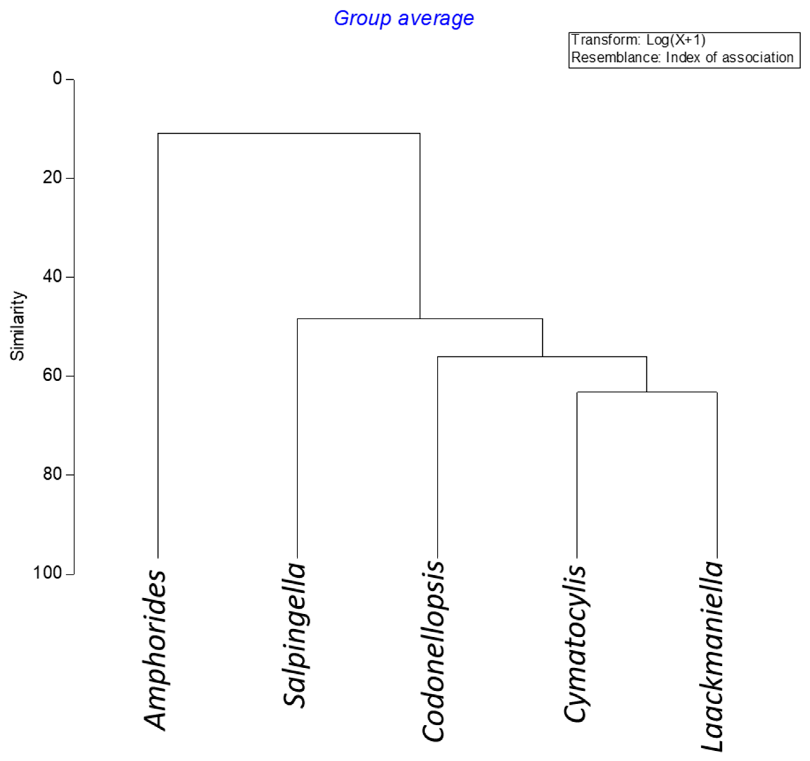
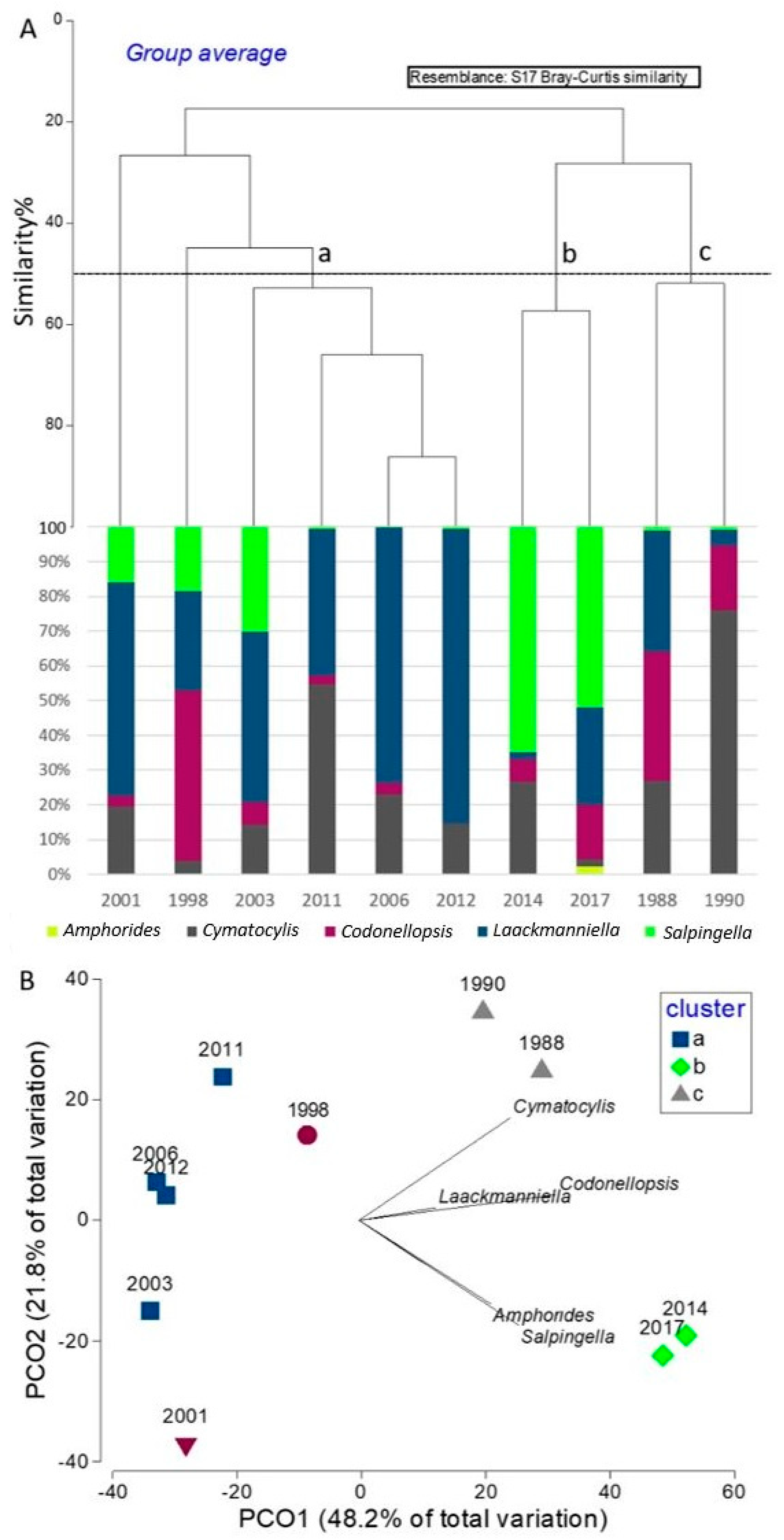
3.3. Tintinnid Community Structure

Analyzing the pattern regulating the genera composition and the genera covariance, PERMANOVA analyses evidence of the influence of the factors “depth layer” in shaping the composition of tintinnids assemblage, in this contest significant (p < 0.05) differences were highlighted among the three layers in the photic zone.

The vertical distribution in the study area, resumed in

Table 3. Vertical distribution and composition of the tintinnids genera reporting average abundance (av.a.), standard deviation (sd), maximum abundance detected (max indL⁻¹), and percentage of presence in the analyzed samples (occurrence %), detected in the three layers defined in the photic zone (< 200 m) during the study period.

	av.a. indL−1			sd			Max indL−1			Occurrence %
	d ≤ 10 m	10 < d ≤ 100 m	100 < d < 200 m	d ≤ 10 m	10 < d ≤ 100 m	100 < d < 200 m	d ≤ 10 m	10 < d ≤ 100 m	100 < d < 200 m	d ≤ 10 m	10 < d ≤ 100 m	100 < d < 200 m
Amphorides	0	5	1	0	21	4	0	133	32	0	8	9
Cymatocylis	50	563	17	131	103	76	1100	470	714	69	80	63
Codonellopsis	58	32	7	150	60	46	1076	300	446	62	49	21
Laackmanniella	33	91	19	71	129	42	413	535	269	63	85	62
Salpingella	127	99	3	452	236	9	3250	975	68	51	50	45

, is characterized by the genera Cymatocylis and Laackmaniella that show the highest occurrence in the three layers. The average abundances and the frequencies of these two genera followed the pattern of total abundance increasing from the surface to the intermediate layer and decreasing in the 100 < d < 200 m layer. The genus Amphorides was absent at 0–10 m while Salpingella and Codonellopsis showed higher abundances and frequencies on the surface following a decreasing trend with the depth.

In regard to the horizontal distribution (

Table 4. Horizontal genera distribution reporting average abundance (av.a.), standard deviation (sd), maximum abundance detected (max indL⁻¹), and percentage of presence in the analyzed samples (occurrence %), detected at less than 5 km from coastline (on), from 5 to 50 km from the coastline (int), at more than 50 km from the coastline (off), during the study period.

	av.a. indL−1			sd			Max indL−1			Occurrence %
	on	int	off	on	int	off	on	int	off	on	int	off
Amphorides	1	2	0	8	12	0	133	83	0	4	6	0
Cymatocylis	34	26	64	79	65	212	442	470	1100	70	56	61
Codonellopsis	15	28	70	50	79	199	446	704	1076	35	43	45
Laackmanniella	27	45	42	57	100	79	346	535	266	67	61	58
Salpingella	12	80	170	68	280	562	716	2782	3250	32	49	71

) the “on/off-shore” factors result is significant in the PERMANOVA analysis (p < 0.05), evidencing different community compositions in the samples collected near the coast (on-shore) from those collected at the intermediate distance (int) or in the open waters (off-shore). In general, the off-shore samples showed higher abundance for the most frequent genera while Amphorides showed higher values in abundance and occurrence near the coast. Cymatocylis and Laackmaniella were more frequent near the coast while Salpingella and Codonellopsis followed the same trend increasing with the coastal distance.

Analyzing the relation between the considered genera and the abiotic factors (temperature and salinity), the vectors presented in Figure 6 showed the biotic variables positively related to temperature, while there is no relationship to salinity.

Spearman correlation index values indicated the significance (p < 0.05) of the correlation between temperature and all the genera, except Amphorides (

Table 5. Spearman correlations index calculated between abiotic factor and tintinnids abundances in the photic layer during the whole study period. Red marked correlations are significant at p < 0.05.

	Amphorides	Cymatocylis	Codonellopsis	Laackmanniella	Salpingella	Tintinnid Abundance
Temperature	0.0558	0.3772	0.4837	0.2516	0.1516	0.4929
Salinity	−0.0838	−0.0305	−0.0976	0.0008	−0.0238	−0.0824

). The negative correlation of Amphorides was probably due to the lower frequency in the observation of this genus. Furthermore, the total abundance of tintinnids showed a higher value in the correlation index with temperature (Table 5).

The cluster analysis, performed on the index of the association matrix among genera (Figure 7), reveals the association between Cymatocylis and Laackmanniella. These genera followed the same trend both in the vertical and horizontal distribution, highlighting similarity in the abundance covariance. Amphorides genus appeared less frequent and rare than the other genera considered in this study and was never detected at the surface layer or in the offshore stations.

3.4. Plurennial Pattern of the Tintinnids Community

Average abundances recorded during years are summarized in Figure 8: in 1988 the abundances were 249 ± 140 indL⁻¹ and then they decreased to 118 ± 90 indL⁻¹ in 1990, these two years with moderate abundances were followed by 5 years with very low abundances (never > 50 ± 87 indL⁻¹) which, however, returned to growth reaching the maximum peaks in 2014 (728 ± 325 indL⁻¹) and 2017 (582 ± 254 indL⁻¹). In general, the carbon content follows the same pattern as the abundance with small discrepancies related to the abundance of genera with larger or smaller dimensions in the tintinnids community.

With reference to the diverse composition recorded in the different years (except 1994, and December samples of the campaigns 1997/98 and 2011/12), the cluster analysis (Figure 9A) and PCO plot (Figure 9B) were performed on the compositions of the populations in the different years and identified three significant groups (PERMANOVA p < 0.05) over the slice of 50% in similarity: in the cluster A, four years (2003, 2006, 2011, 2012) were characterized in the simper analysis output (

Table 6. SIMPER analysis within cluster performed on the genera abundance matrix. Average abundance (av.a.), average similarity (av.sim.), contribution % (contrib. %), cumulative % (cum. %).

Cluster A
Average similarity: 62.70
	av.a.	av.sim.	contrib.%	cum.%
Laackmanniella	24.64	46.98	74.94	74.94
Cymatocylis	11.74	13.62	21.72	96.66
Cluster B
Average similarity: 57.35
	av.a.	av.sim.	contrib.%	cum.%
Salpingella	386.69	45.99	80.20	80.20
Codonellopsis	68.86	7.20	12.55	92.75
Cluster C
Average similarity: 51.87
	av.a.	av.sim.	contrib.%	cum.%
Cymatocylis	78.28	36.51	70.40	70.40
Codonellopsis	57.18	11.92	22.99	93.39

) by highest relative abundances of the genera Laackmaniella and Cymatocylis. In cluster B, the years 2014 and 2017 were characterized by the highest abundances and a high percentage of genera Salpingella and Codonellopsis within the population; finally, cluster C (1988 and 1990), was characterized by intermediate abundances with high percentages of Cymatocylis and Codonellopsis. The years 1998 (showing the highest percentage in Codonellopsis) and 2001 (showing the lowest total abundances) were not grouped in any cluster.

4. Discussion

Over eleven summer expeditions from 1988 to 2017 we have detected only nine tintinnids species belonging to five genera, therefore confirming the low tintinnids diversity in TNB winter polynya area, and in the Antarctic waters in general [41,54,55,56,57]. Previously, in TNB a richer list comprising 14 species was reported [58]. This difference is mainly due to a recent taxonomic rearrangement [50]. Indeed, Cymatocylis ecaudata Kofoid and Campbell 1929 detected in [54] is now a synonym of C. drygalskii and C. folliculus Kofoid and Campbell 1929 as well as of C. nobilis. Cymatocylis conica (Laackmann) Kofoid and Campbell 1929 and C. flava Laackmann 1910 are grouped into the species C. vanhoeffeni, while C. glans Kofoid and Campbell 1929 and C. subconica Kofoid and Campbell 1929 are grouped into the species C. cristallina. Laackmanniella prolongata (Laackmann) Kofoid and Campbell 1929 is now a synonym of L. naviculaefera [50].

Excluding 1994, which had only one station, on average three species (C. drygalskii, C. gaussi, and L. naviculaefera) were recorded for each year of the study period. These species are common in the Southern Ocean [59] and they are often dominant in coastal tintinnid communities [26]. In TNB polynya, they can be considered key species and their presence and fluctuation in abundance should be considered an important signal of possible changes in the whole plankton community.

Only in 1997/98 and 2011/12, we sampled in December, January, and February. On these two occasions, we recorded fewer species and lower abundances in early December compared to the January–February period, confirming a seasonal pattern and late development of the tintinnid community observed [40,60]. In December 1997 and 2011, tintinnids’ community was particularly scarce, whereas a significant increase over the period January–February was recorded.

The phytoplankton community in the Ross Sea is dominated by the haptophytes Phaeocystis antarctica and diatoms, and it shows different temporal and spatial patterns [18]. In TNB, the other functional groups (dinoflagellates, cryptophytes, cyanophytes, chlorophytes) are poorly represented and are considered to have a minor role in the Antarctic food web [18,20,61,62]. Generally, in the TNB during December there is a Phaeocystis-dominated inshore area and a small-diatoms-dominated community at the retreating ice edge. Later in the season, the herbivorous food web is more active, whereas in late February the consumers’ community shifts toward smaller-sized organisms (namely protists), and the food web is considered mistivourus [60]. Considering this as the usual seasonal food web structure development in the study area [55,63,64], we decided to omit December samples from the multiyear comparisons (1994, 1997, and 2011).

A clear decreasing tintinnids abundance till 2012 is evident when considering the January–February annual average, which started during the first sampled year (1988) and dramatically dropped in January 2001. The general decreasing trend (despite the limitation due to the data collected over a long period and in different sites) might be due to the analogous decreasing trend of phytoplankton biomass, which was detected from 1997 onward [11,65]. In many studies, it has been demonstrated that microzooplankton (and consequently tintinnids) abundances are tightly coupled with chlorophyll concentration [55,57,58,66,67,68,69]. Arrigo and van Dijken [11] suggested that chlorophyll concentrations are mainly controlled by ice coverage. Low chlorophyll concentrations are measured in areas with less extension of ice-free waters. Consequently, we can assume that the increasing ice coverage since 1978 reported by Stammerjohn and Smith [69] could have affected the phytoplankton biomass, which in turn controls micrograzers (namely protists) abundances. Particularly in the 1997–1998 and 2000–2001 austral summers, chlorophyll a concentration was low over the whole season, and the phytoplankton blooms were less extended and delayed by almost two months, peaking only in February [11]. In addition to the interannual fluctuation, which is probably related to ENSO (El Niño-Southern Oscillations) oscillations [11], the 2000–2001 austral summer was impacted by the drifting of the immense iceberg B 15, which impeded the normal circulation pattern in the western Ross Sea, thus strongly affecting primary production and higher trophic levels through a cascading effect [69]. In the austral summer 2002–2003 Harangozo and Connolley [70] registered the minimum extent of open water in the Ross Sea, which again could have lowered primary production and consequently phytoplankton biomass. Moreover, minimum values of tintinnids biomass were detected in 2001 and they remained very low until 2014.

On the contrary, the increase in abundance in 2014 and 2017 can be related to the increase in the surface layer temperature, which may cause an increase in the buoyancy of the surface waters relative to the underlying layer and consequently decrease the vertical exchange.

The timing and magnitude of primary productivity in the Ross Sea has been changing during the last years, with a general increase in the area of the Ross Sea polynya [71,72]. These changes may have influenced the tintinnid community. In the last period (2014 and 2017) we noticed an increase in the abundance of the dominant species (C. drygalskii, C. gaussi, and L. naviculaefera), and of the Salpingella genus. Moreover, A. laackmanni was detected for the first time in the area. Salpingella and A. laackmanni are two taxa not peculiar to Antarctica but widespread in the Southern Ocean [41,59] and they both present a similar oral diameter (LOD). The variation in the LOD of tintinnids can reflect the size spectrum of food items available. Previous studies showed that the species assemblage of the Southern Ocean appears to be distributed bimodally with peaks at about 45 and 120 µm, suggesting that most species likely use prey of 10–15 µm or 30 µm [59]. The most abundant species detected in this study (C. drygalskii, C. gaussi, and L. naviculaefera) fall perfectly into these two classes and the recent increase in small diatoms in TNB [20] could explain their increase in abundance. On the contrary, the Salpingella genus and A. laackmanni present both a smaller oral diameter (LOD between 15 to 20 µm), and they are supposed to feed on prey < 10 µm. The TNB community size structure in 2017, together with the high percentage of microphytoplankton (39%), showed high values also for nano-phytoplankton (39%) and pico-phytoplankton (22%) [73] as possible prey for tintinnids with smaller LOD.

The different abundances of tintinnids in TNB can be linked to the higher biomass of diatoms reported near the coastline [20,26,73]. Previous studies showed L. naviculaefera and C. gaussi more abundant in the stations close to the coast and Cymatocylis in the offshore stations [58]. Additionally, our results showed that L. naviculaefera was more abundant in the stations closer to the coast, while other species showed different tendencies. We speculate that these differences are due to the small sampling scale employed in our study, which means that in general our samples can be compared to the coastal area samples in other studies, (e.g., [73]).

During the summer the area presents a typical vertical structure, with the DSW at the bottom and the lightest Antarctic surface water (AASW) occupying the top 100 m layer [73]. The higher abundance of tintinnids in the layer 0–100 m is confirmed also by previous studies where Salpingella, C. gaussi, and L. naviculaefera were present in higher abundance at the surface, while C. drygalskii and C. convallaria were mainly found at intermediate depths [42,74]. Liang et al. [42] showed that A. laackmanni had no clear depth pattern, notwithstanding in our study this species was mainly found in the 10–100 m layer.

5. Conclusions

During our observation period, the tintinnids’ community in TNB polynya was characterized by a low species richness, mainly dominated by large-mouthed species endemic to the area. Three species (C. drygalskii, C. gaussi, and L. naviculaefera) appeared to be keystone species for their persistent occurrence and relevant abundance. In 2014 and 2017, the surface temperature in TNB increased showing a clear positive correlation with the abundance of the tintinnids, whereas the salinity did not show any relationship with the abundance. In this last period, the increase in the tintinnid key species abundance and the first appearance of cosmopolitan tintinnid A. laackmanni were detected.

Recent studies show that phytoplankton assemblage will likely increase in the future due to changes in summer sea ice concentrations; therefore, studies on tintinnids as grazers of nano and micro-phytoplankton, and as prey for krill and salps, are key to understand the trophic interactions at the base of the Southern Ocean ecosystem. A modification in tintinnids’ abundance and composition can influence the entire Antarctic food web, changing the efficiency of energy between the different trophic levels. Long-term studies on evolution of tintinnids population can be used as a monitor for environmental changes and as a useful approach for understanding the evolution of the whole plankton community in TNB polynya.

References

1. Jacobs, S.S.; Giulivi, C.F.; Dutrieux, P. Persistent Ross Sea freshening from imbalance West Antarctic ice shelf melting. J. Geophys. Res. Oceans 2022, 127, e2021JC017808. [Google Scholar] [CrossRef]
2. Castagno, P.; Capozzi, V.; DiTullio, G.R.; Falco, P.; Fusco, G.; Rintoul, S.R.; Spezie, G.; Budillon, G. Rebound of shelf water salinity in the Ross Sea. Nat. Commun. 2019, 10, 5441. [Google Scholar] [CrossRef]
3. Silvano, A.; Foppert, A.; Rintoul, S.R.; Holland, S.R.; Tamura, T.; Kimura, N.; Castagno, P.; Falco, P.; Budillon, G.; Haumann, F.A.; et al. Recent recovery of Antarctic Bottom Water formation in the Ross Sea driven by climate anomalies. Nat. Geosci. 2020, 10, 5441. [Google Scholar] [CrossRef]
4. Lecomte, O.; Goosse, H.; Fichefet, T.; de Lavergne, C.; Barthélemy, A.; Zunz, V. Vertical ocean heat redistribution sustaining sea-ice concentration trends in the Ross Sea. Nat. Commun. 2017, 8, 258. [Google Scholar] [CrossRef] [Green Version]
5. Jacobs, S.S.; Giulivi, C.F. Large multidecadal salinity trends near the Pacific-Antarctic continental margin. J. Clim. 2010, 23, 4508–4524. [Google Scholar] [CrossRef]
6. Bromwich, D.H.; Kurtz, D.D. Katabatic wind forcing of the Terra Nova Bay polynya. J. Geophys. Res. 1984, 89, 3561–3572. [Google Scholar] [CrossRef]
7. Kurtz, D.D.; Bromwich, D.H. A recurring atmospherically-forced polynya in Terra Nova Bay. In Oceanology of the Antarctic Continental Shelf; Jacobs, S.S., Ed.; Antarctic Research Series; American Geophysical Union: Washington, DC, USA, 1985; Volume 43, pp. 177–201. [Google Scholar]
8. Kern, S. Wintertime Antarctic coastal polynya area: 1992–2008. Geophys. Res. Lett. 2009, 36, 1–5. [Google Scholar] [CrossRef]
9. Rusciano, E.; Budillon, G.; Fusco, G.; Spezie, G. Evidence of atmosphere–sea ice–ocean coupling in the Terra Nova Bay polynya (Ross Sea—Antarctica). Cont. Shelf Res. 2013, 61–62, 112–124. [Google Scholar] [CrossRef] [Green Version]
10. Budillon, G.; Fusco, G.; Spezie, G. A study of surface heat fluxes in the Ross Sea (Antarctica). Antarct. Sci. 2000, 12, 243–254. [Google Scholar] [CrossRef]
11. Arrigo, K.R.; van Dijken, G.L. Annual changes in sea-ice, chlorophyll a, and primary production in the Ross Sea, Antarctica. Deep-Sea Res. 2004, 51, 117–138. [Google Scholar] [CrossRef]
12. Arrigo, K.R.; van Dijken, G.L. Phytoplankton dynamics within 37 Antarctic coastal polynya systems. J. Geophys. Res. 2003, 108, 3271. [Google Scholar] [CrossRef]
13. Arrigo, K.R.; Worthen, D.L.; Schnell, A.; Lizotte, M.P. Primary production in Southern Ocean waters. J. Geophys. Res. 1998, 103, 587–600. [Google Scholar] [CrossRef]
14. DiTullio, G.R.; Smith, W.O., Jr. Spatial patterns in phytoplankton biomass and pigment distributions in the Ross Sea. J. Geophys. Res. 1996, 101, 467–478. [Google Scholar] [CrossRef]
15. Smith, W.O., Jr.; Gordon, L.I. Hyperproductivity of the Ross Sea (Antarctica) polynya during austral spring. Geophys. Res. Lett. 1997, 24, 233–236. [Google Scholar] [CrossRef]
16. Smith, W.O.; Marra, J.; Hiscock, M.R.; Barber, R.T. The seasonal cycle of phytoplankton biomass and primary productivity in the Ross Sea. Antarctica. Deep-Sea Res. II 2000, 47, 3119–3140. [Google Scholar] [CrossRef]
17. Nuccio, C.; Innamorati, M.; Lazzara, L.; Mori, G.; Massi, L. Spatial and temporal distribution of phytoplankton assemblages in the Ross Sea. In Ross Sea Ecology; Faranda, F.M., Guglielmo, L., Ianora, A., Eds.; Springer: Berlin, Germany, 2000; pp. 231–245. [Google Scholar]
18. Smith, W.O., Jr.; Ainley, D.G.; Arrigo, K.R.; Dinniman, M.S. The Oceanography and Ecology of the Ross Sea. Ann. Rev. Mar. Sci. 2014, 6, 469–487. [Google Scholar] [CrossRef] [Green Version]
19. Xu, K.; Fu, F.X.; Hutchins, D.A. Comparative responses of two dominant Antarctic phytoplankton taxa to interactions between ocean acidification, warming, irradiance, and iron availability. Limnol. Oceanogr. 2014, 59, 1919–1931. [Google Scholar] [CrossRef]
20. Mangoni, O.; Saggiomo, V.; Bolinesi, F.; Margiotta, F.; Budillon, G.; Cotroneo, Y.; Misic, C.; Rivaro, P.; Saggiomo, M. Phytoplankton blooms during austral summer in the Ross Sea, Antarctica: Driving factors and trophic implications. PLoS ONE 2017, 12, e0176033. [Google Scholar] [CrossRef] [Green Version]
21. Bjørnsen, P.; Kuparinen, J. Growth and herbivory by heterotrophic dinoflagellates in the Southern Ocean, studied by microcosm experiments. Mar. Biol. 1991, 109, 397–405. [Google Scholar] [CrossRef]
22. Kuparinen, J.; Bjørnsen, P. Bottom-up and top-down controls of the microbial food web in the Southern Ocean: Experiments with manipulated microcosms. Polar Biol. 1992, 12, 189–195. [Google Scholar] [CrossRef]
23. Sherr, E.B.; Sherr, B.E. Significance of predation by protists in aquatic microbial food webs. Antonie Van Leeuwenhoek Inter. J. Gen. Mol. Microbiol. 2002, 81, 293–308. [Google Scholar]
24. Calbet, A.; Landry, M.R. Phytoplankton growth, microzooplankton grazing, and carbon cycling in marine system. Limnol. Oceanogr. 2004, 49, 51–57. [Google Scholar] [CrossRef] [Green Version]
25. Schmoker, C.; Hernández-León, S.; Calbet, A. Microzooplankton grazing in the oceans: Impacts, data variability, knowledge gaps and future directions. J. Plankton Res. 2013, 35, 691–706. [Google Scholar] [CrossRef]
26. Fonda Umani, S.; Monti, M.; Bergamasco, A.; Cabrini, M.; De Vittor, C.; Burba, N.; Del Negro, P. Plankton community structure and dynamics versus physical structure from Terra Nova Bay to Ross Ice Shelf (Antarctica). J. Mar. Syst. 2005, 55, 31–46. [Google Scholar] [CrossRef]
27. Dolan, J.R. Morphology and ecology in tintinnid ciliates of the marine plankton: Correlates of lorica dimensions. Acta Protozool. 2010, 49, 235–244. [Google Scholar]
28. Boltovskoy, D.; Dinofrio, E.O.; Alder, A.A. Intraspecific variability in Antarctic tintinnids: The Cymatocylis affinis/convallaria species group. J. Plankton Res. 1990, 12, 403–413. [Google Scholar] [CrossRef]
29. Williams, R.; McCall, H.; Pierce, R.W.; Turner, J.T. Speciation of the tintinnid genus Cymatocylis by morphometric analysis of the loricae. Mar. Ecol. Prog. Ser. 1994, 107, 263–272. [Google Scholar] [CrossRef]
30. Wasik, A.; Mikołajczyk, E. Annual cycle of tintinnids in Admiral Bay with an emphasis on seasonal variability in Cymatocylis affinis/convallaria lorica morphology. J. Plankton Res. 1994, 16, 1–8. [Google Scholar] [CrossRef]
31. Kruse, S.; Jansen, S.; Krägefsky, S.; Bathman, U. Gut content analysis of three dominant Antarctic copepod species during an induced phytoplankton bloom EIFEX (European iron fertilization experiment). Mar. Ecol. 2009, 30, 301312. [Google Scholar] [CrossRef]
32. Mauchline, J. The biology of mysids and euphausiids. In Advances in Marine Biology 18; Academic Press: London, UK, 1980. [Google Scholar]
33. Buck, K.R.; Garrison, D.L.; Hopkins, T.L. Abundance and distribution of tintinnid ciliates in an ice edge zone during the austral autumn. Antarct. Sci. 1992, 4, 398. [Google Scholar] [CrossRef]
34. Hopkins, T.L. Midwater food web in McMurdo sound, Ross Sea, Antarctica. Mar. Biol. 1987, 96, 93106. [Google Scholar] [CrossRef]
35. Kellermann, A. Food and feeding ecology of postlarval and juvenile Pleurogramma antarcticum (Pisces; Notothenioidei) in the seasonal pack ice zone off the Antarctic Peninsula. Polar Biol. 1987, 7, 307315. [Google Scholar] [CrossRef]
36. Laackmann, H. Antarktische Tintinninen. Zool. Anz. 1907, 3, 235–239. [Google Scholar]
37. Laackmann, H. Die Tintinnodeen der Deutschen Südpolar-Expedition 1901–1903. Dtsch. Südpolar-Exped. 1903, 1910, 341–496. [Google Scholar]
38. Jiang, Y.; Yang, E.J.; Kim, S.Y.; Kim, Y.-N.; Lee, S.H. Spatial patterns in pelagic ciliate community responses to various habitats in the Amundsen Sea (Antarctica). Prog. Oceanogr. 2014, 128, 49–59. [Google Scholar] [CrossRef]
39. Jiang, Y.; Liu, Q.; Yang, E.J. Pelagic ciliate communities within the Amundsen Sea polynya and adjacent sea ice zone, Antarctica. Deep Sea Res. II 2016, 123, 69–77. [Google Scholar] [CrossRef]
40. Monti-Birkenmeier, M.; Diociaiuti, T.; Fonda Umani, S.; Meyer, B. Microzooplankton composition in the winter sea ice of the Weddell Sea. Antarct. Sci. 2017, 29, 299–310. [Google Scholar] [CrossRef]
41. Monti-Birkenmeier, M.; Diociaiuti, T.; Badewien, T.H.; Schulz, A.C.; Friedrichs, A.; Meyer, B. Microzooplankton composition in the Antarctic Peninsula region, with an emphasis on tintinnids. Polar Biol. 2021, 44, 1749–1764. [Google Scholar] [CrossRef]
42. Liang, C.; Li, H.; Dong, Y.; Zhao, Y.; Tao, Z.; Li, C.; Zhang, W.; Gregori, G. Planktonic ciliates in different water masses in open waters near Prydz Bay (East Antarctica) during austral summer, with an emphasis on tintinnid assemblages. Polar Biol. 2018, 41, 2355–2371. [Google Scholar] [CrossRef]
43. Liang, C.; Li, H.B.; Zhang, W.C.; Tao, Z.; Zhao, Y. Changes in tintinnid assemblages from Subantarctic zone to Antarctic zone along transect in Amundsen Sea (west Antarctica) in early austral autumn. J. Ocean Univ. China 2020, 19, 339–350. [Google Scholar] [CrossRef]
44. Utermöhl, H. Zur Vervollkommung der quantitativen Phytoplankton-Methodik. Mitt. Int. Theor. Angew. Limnol. 1958, 9, 1–38. [Google Scholar]
45. Brandt, K. Die Tintinnodeen der Plankton-Expedition. Tefelerklarungen nebts kurzer Diagnose der neuen Arten. In Ergebn. Atlant. Ozean Planktonexpedition; Hensen, V., Ed.; Humboldt-Stift: Kiel und Leipzig, Germany, 1906; Volume 3, pp. 1–33. [Google Scholar]
46. Brandt, K. Die Tintinnodeen der Plankton-Expedition. Sistematischer Teil. In Ergebn. Atlant. Ozean Planktonexpedition; Hensen, V., Ed.; Humboldt-Stift: Kiel und Leipzig, Germany, 1907; Volume 3, pp. 1–488. [Google Scholar]
47. Kofoid, C.A.; Campbell, A.S. A conspectus of the marine and fresh-water Ciliata belonging to the suborder Tintinnoinea with descriptions of new species principally from the Agassiz Expedition to the eastern tropical Pacific, 1904–1905. Univ. Calif. Publ. Zool. 1929, 34, 1–403. [Google Scholar]
48. Kofoid, C.A.; Campbell, A.S. Reports on the scientific results of the expedition to the Eastern Tropical Pacific. The Ciliata: The Tintinnoinea. Bull. Mus. Comp. Zool. Harvard Univ. 1939, 84, 1–473. [Google Scholar]
49. Alder, V.A. Tintinnoinea. In South Atlantic Zooplankton; Boltovskoy, D., Ed.; Backhuys: Leiden, The Netherlands, 1999; pp. 321–384. [Google Scholar]
50. Petz, W. Ciliates. In Antarctic Marine Protists; Scott, F.J., Marchant, H.J., Eds.; Camberra ABRS: Hobart, Australia, 2005; pp. 347–448. [Google Scholar]
51. Verity, P.G.; Langdon, C. Relationship between lorica volume, carbon, nitrogen, and ATP content of tintinnids in Narragansett Bay. J. Plankton Res. 1984, 6, 859–868. [Google Scholar] [CrossRef]
52. Bray, J.R.; Curtis, J.T. An ordination of upland forest communities of southern Wisconsin. Ecol. Monogr. 1957, 27, 325–349. [Google Scholar] [CrossRef]
53. Clarke, K.R.; Gorley, R.N. Getting Started with PRIMER v7. PRIMER-E; Plymouth Marine Laboratory: Plymouth, UK, 2015. [Google Scholar]
54. Pierce, R.W.; Turner, J.T. Global biogeography of marine tintinnids. Mar. Ecol. Progr. Ser. 1993, 94, 11–26. [Google Scholar] [CrossRef]
55. Monti, M.; Fonda Umani, S. Distribution of the main microzooplankton taxa in the Ross Sea (Antarctica): Austral summer 2004. In Ross Sea Ecology; Faranda, F.M., Guglielmo, L., Ianora, A., Eds.; Springer: Berlin, Germany, 2000; pp. 275–289. [Google Scholar]
56. Gowing, M.M.; Garrison, D.L. Larger microplankton in the Ross Sea: Abundance, biomass and flux in the austral summer. In Biogeochemistry of the Ross Sea; DiTullio, G.R., Dunbar, R.B., Eds.; Wiley: Hoboken, NJ, USA, 2003; pp. 243–260. [Google Scholar]
57. Thompson, G.A.; Alder, V.A. Patterns in tintinnid species composition and abundance in relation to hydrological conditions of the southwestern Atlantic during austral spring. Aquat. Microb. Ecol. 2005, 40, 85–101. [Google Scholar] [CrossRef] [Green Version]
58. Monti, M.; Fonda Umani, S. Tintinnids in Terra Nova Bay—Ross Sea during two austral summer (1987/88 and 1989/90). Acta Protozool. 1995, 34, 193–201. [Google Scholar]
59. Dolan, J.R.; Pierce, R.W.; Yang, E.J.; Kim, S.Y. Southern Ocean biogeography of tintinnid ciliates of the marine plankton. J. Eukaryot. Microbiol. 2012, 59, 511–519. [Google Scholar] [CrossRef]
60. Fonda Umani, S.; Accornero, A.; Budillon, G.; Capello, M.; Tucci, S.; Cabrini, M.; Del Negro, P.; Monti, M.; De Vittor, C. Particulate matter and plankton dynamics in the Ross Sea Polynya of Terra Nova Bay during the Austral Summer 1997/98. J. Mar. Syst. 2002, 36, 29–49. [Google Scholar] [CrossRef]
61. Andreoli, C.; Tolomio, C.; Moro, I.; Radice, M.; Moschin, E.; Bellato, S. Diatoms and dinoflagellates in Terra Nova Bay (Ross Sea-Antarctica) during austral summer 1990. Polar Biol. 1995, 15, 465–475. [Google Scholar] [CrossRef]
62. Arrigo, K.R.; DiTullio, G.R.; Dunbar, R.B.; Robinson, D.H.; van Woert, M.; Worthen, D.L.; Denise, L.W.; Lizotte, M.P. Phytoplankton taxonomic variability in nutrient utilization and primary production in the Ross Sea. J. Geophys. Res. 2000, 105, 8827–8846. [Google Scholar] [CrossRef]
63. Garrison, D.L.; Mathot, S.; Gowing, M.M.; Kunze, H.; Lessard, E.J. Phytoplankton and microzooplankton community structure in the Ross Sea polynya: November and December 1994. Antarct. J. U. S. 1995, 30, 212–214. [Google Scholar]
64. Seibel, B.A.; Dierssen, H.M. Cascading trophic impacts of reduced biomass in the Ross Sea, Antarctica: Just a tip of the iceberg? Biol. Bull. 2003, 205, 93–97. [Google Scholar] [CrossRef] [Green Version]
65. Stoecker, D.K.; Putt, M.; Moisan, T. Nano- and microplankton dynamics during the spring Phaeocystis sp. bloom in McMurdo Sound, Antarctica. J. Mar. Biol. Assoc. U. K. 1995, 75, 815–832. [Google Scholar] [CrossRef]
66. Gowing, M.M.; Garrison, D.L. Austral winter distribution of large tintinnid and large sarcodinid protozooplankton in the ice-edge zone of the Weddel/Scotia Seas. J. Mar. Syst. 1991, 2, 131–141. [Google Scholar] [CrossRef]
67. Hansen, P.J. Dinophysis—A planktonic dinoflagellate genus which can act as a prey and a predator of a ciliate. Mar. Ecol. Progr. Ser. 1991, 69, 201–204. [Google Scholar] [CrossRef]
68. Alder, V.A.; Boltovskoy, D. The ecology of larger microzooplankton in the Weddell-Scotia Confluence Area: Horizontal and vertical distribution patterns. J. Mar. Res. 1993, 51, 323–344. [Google Scholar] [CrossRef]
69. Stammerjohn, S.E.; Smith, R.C. Opposing Southern Ocean climate patterns as revealed by trends in regional sea ice coverage. Clim. Change 1997, 37, 617–639. [Google Scholar] [CrossRef]
70. Harangozo, S.A.; Connolley, W.M. The role of the atmospheric circulation in the record minimum extent of open water in the Ross Sea in the 2003 austral summer. Atmosphere-Ocean 2006, 44, 83–97. [Google Scholar] [CrossRef] [Green Version]
71. Montes-Hugo, M.A.; Yuan, X. Climate patterns and phytoplankton dynamics in Antarctic latent heat polynyas. J. Geophys. Res. 2012, 117, C05031. [Google Scholar] [CrossRef] [Green Version]
72. Schine, C.M.S.; van Dijken, G.L.; Arrigo, K.R. Spatial analysis of trends in primary production and relationship with large-scale climate variability in the Ross Sea, Antarctica (1997–2013). J. Geophys. Res. Oceans 2016, 121, 368–386. [Google Scholar] [CrossRef] [Green Version]
73. Bolinesi, F.; Saggiomo, M.; Ardini, F.; Castagno, P.; Cordone, A.; Fusco, G.; Rivaro, P.; Saggiomo, V.; Mangoni, O. Spatial-related community structure and dynamics in phytoplankton of the Ross Sea, Antarctica. Front. Mar. Sci. 2020, 7, 1092. [Google Scholar] [CrossRef]
74. Boltovskoy, D.; Adler, V.A. Microzooplankton and tintinnid species-specific assemblage structures: Patterns of distribution and year-to-year variations in the Weddell Sea (Antarctica). J. Plankton Res. 1992, 14, 1405–1423. [Google Scholar] [CrossRef]
Figure 1. Survey stations in the Ross Sea polynya in the different years. Mario Zucchelli Station (MZS).
Diversity 14 00604 g001
Figure 2. Average abundance of tintinnids (indL−1) and average tintinnids carbon content (µgCL−1) in the study area detected in the totality of early summer samples (early: December) and late summer samples (late: January and February); bars represent standard deviation (sd); early n = 39, late n = 282.
Diversity 14 00604 g002
Figure 3. Average abundance of tintinnids (indL−1) and average tintinnids carbon content (µgCL−1) in the study area detected in the totality of the photic zone (photic < 200 m) and in the aphotic zone (aphotic ≥ 200 m); bars represent standard deviation (sd); photic n = 272, aphotic n = 49.
Diversity 14 00604 g003
Figure 4. Average abundance distribution of tintinnids (indL−1) and carbon content (µgCL−1) in the three layers defined in the photic zone (<200 m); bars represent standard deviation (sd); d ≤ 10 m, n = 99; 10 < d ≤ 100 m, n = 74; 100 < d < 200 m, n = 99.
Diversity 14 00604 g004
Figure 5. The most representative species detected in the study area. (A) Cymatocylis drygalskii, (B) Laackmanniella naviculaefera, (C) Codenollepsis gaussi, (D) Cymatocylis vanhöffeni.
Diversity 14 00604 g005
Figure 6. nMDS on community structure reporting vectors of abiotic (red) and biotic (black) variables, only the biotic ones contribute to the distribution while temperature (T) and salinity (S) vectors are plotted in order to show the possible relationship.
Diversity 14 00604 g006
Figure 7. Cluster analysis on the index of association among genera.
Diversity 14 00604 g007
Figure 8. Annual average abundance (indL−1) and annual average carbon content (µgCL−1) of tintinnids dets. Sample numbers for each year are provided in Table S2.
Diversity 14 00604 g008
Figure 9. Community composition and similarity recorded during years, cluster analysis (A) and PCO (B) were performed on Bray-Curtis similarity matrix.
Diversity 14 00604 g009