Article

Modeling the Potential Distribution of Two Species of Shrews (Chodsigoa hypsibia and Anourosorex squamipes) under Climate Change in China

1
Anhui Provincial Key Laboratory of the Conservation and Exploitation of Biological Resources, College of Life Sciences, Anhui Normal University, Wuhu 241000, China
2
Collaborative Innovation Center of Recovery and Reconstruction of Degraded Ecosystem in Wanjiang Basin Co-Founded by Anhui Province and Ministry of Education, School of Ecology and Environment, Anhui Normal University, Wuhu 241002, China
3
State Key Laboratory of Genetic Resources and Evolution, Kunming Institute of Zoology, Chinese Academy of Sciences, Kunming 650204, China
*
Author to whom correspondence should be addressed.
Diversity 2022, 14(2), 87; https://doi.org/10.3390/d14020087
Submission received: 15 November 2021 / Revised: 25 January 2022 / Accepted: 26 January 2022 / Published: 27 January 2022

Abstract

:
Understanding how the direct and indirect effects of climate change may affect species distributions is a key topic in ecology. We used maximum entropy models to explore the distribution of two species of shrews (Chodsigoa hypsibia and Anourosorex squamipes) in China and analyzed the main environmental factors affecting their current distribution and potential distribution changes under two future climate scenarios. The results showed that the major environmental factors determining the current distribution of C. hypsibia were the mean temperature of the coldest quarter (contributing 47.4%), annual mean temperature (contributing 24.7%), precipitation of the driest quarter (contributing 21.1%) and isothermality (contributing 6%). Annual precipitation (contributing 42.9%), precipitation of the driest month (contributing 28.1%), annual mean temperature (contributing 14.8%) and temperature seasonality (contributing 12.6%) had the highest contributions to the distribution of A. squamipes. Under future climate scenarios, the suitable habitat range of C. hypsibia increased while that of A. squamipes decreased. These findings demonstrate that different small mammal species respond differently to climate change.

1. Introduction

Natural populations respond to global climate change by changing their geographic distribution and timing of growth and reproduction, which, in turn, change the composition of communities and the nature of species interactions. Many populations’ reactions, however, are likely to be insufficient to deal with the speed and extent of climate change, leaving them vulnerable to population decline and extinction [1]. For example, climate change could result in the extinction of a quarter of all plants and animals if greenhouse gas emissions are not curbed [2]. Thus, it is an ecological priority to understand how species distributions may be directly or indirectly affected by climate change [3]. Future distributions are usually estimated by relating climatic conditions with the current distribution ranges of key species and projecting future conditions [4]. These species distribution models (SDMs) are useful tools for deciphering the elements that influence the prospective distributions of several organisms at various scales [5]. The maximum entropy approach (MaxEnt) [6] has been widely used in biological invasion predictions [7], habitat prediction for endangered animals [8], forest fire prediction [9], responses of species to climate change [10] and prediction of potential threats from pest species [11], due to its good simulation accuracy [12].
Small mammals such as shrews play a significant role in many ecological systems since they are the primary prey of many mammals, birds, and reptiles and can influence the makeup of vegetation communities through seed dispersal [13,14]. However, the influence of climate change on small mammals has been difficult to predict because of their narrow and often discontinuous ranges and low dispersal ability [15]. Shrews, one of the smallest mammals in the world, have unique physiological and ecological characteristics that are sensitive to climate change [16]. Studies show shrews are highly dependent on their environment [17] and do not migrate over long distances [18], making them ideal for exploring species interactions with the environment. Shrews are also very sensitive to severe environmental conditions due to thermal inertia and lower resistance to famine, owing to their fast metabolism and small body size [16]. As a result, shrews should be extremely sensitive to future temperature or precipitation changes that may be beyond their physiological tolerances, causing range shifts or contractions [15].
Despite Chodsigoa hypsibia and Anourosorex squamipes being among the most widely distributed shrews in China, an extremely complex topography and the high variation in their habitats have hindered ecological research into their current and future distributions. C. hypsibia has a wide distribution in central and southwestern China, with the main population distributed in the Hengduan Mountains, which is an endemic species in China [19]. On the other hand, A. squamipes is primarily distributed in southwestern China, but also occur in northern Laos, northern Vietnam, northern Thailand and northeast Myanmar, where it can be found at elevations from 300 to 4000 m and latitudes from 18 to 35 degrees north. A. squamipes is good at digging and inhabit diverse habitats, including forests, farmlands and wastelands, and has highly diverse and flexible diets that include insects, annelids and plants [20]. Compared to C. hypsibia, A. squamipes has a wide ecological range and is adapted to different habitats and altitudes, with C. hypsibia occurring in more complex mountain environments. Therefore, we chose these two species for two reasons: (1) C. hypsibia and A. squamipes are among the most widely distributed insectivore in China; and (2) C. hypsibia and A. squamipes have different ecological amplitude. The objective of this study was to explore how climate change affected the distribution of them.
The distribution of C. hypsibia and A. squamipes has been studied widely during the last thirty years [20,21]. In this study, we used MaxEnt modeling to predict the distributions and main environmental factors affecting the current distribution of the two species, as well as explore their distribution changes under two future climate change scenarios, using an extensive dataset of georeferenced occurrence records from recent surveys.

2. Materials and Methods
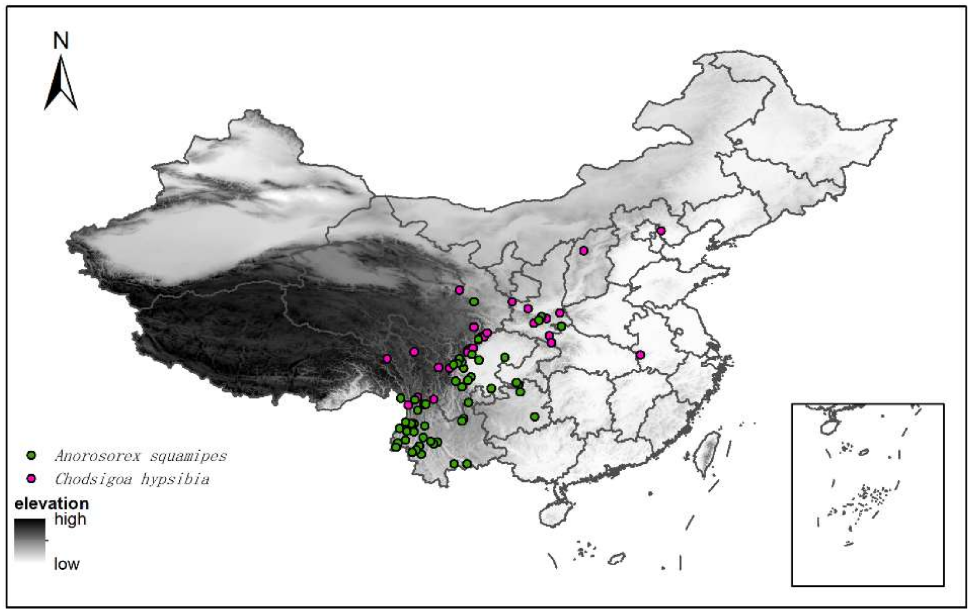
2.1. Sample Data

To obtain occurrence records for C. hypsibia and A. squamipes over their ranges, we inspected specimens deposited at Kunming Institute of Zoology (KIZ), Chinese Academy of Sciences, and complemented them with data from the Global Biodiversity Information Facility (GBIF, https://www.gbif.org/ (accessed on 4 December 2021)). Records with no geographical coordinates were excluded and those remaining were visually inspected for errors. Ambiguous or duplicate records were further removed to reduce bias caused by spatial autocorrelation. Duplicates were deleted within each grid cell (5 km × 5 km), due to the SDM analyses, to reduce the bias caused by spatial autocorrelation. Finally, a total of 30 and 50 documented presence records of C. hypsibia and A. squamipes, respectively, were obtained for constructing the models (Figure 1, Table S1).

2.2. Current and Future Environmental Variables

To predict the current and future distributions, we selected a total of 20 environmental variables for the model input: elevation (30 m resolution) and 19 bioclimatic variables (30 m resolution). The 19 bioclimatic variables and elevation were obtained from WorldClim (http://www.worldclim.org/bioclim (accessed on 4 December 2021) (Table 1) [22]. The climate variables are important biological parameters that affect the species survival. They are generated by monthly temperature and rainfall quantity, including annual trends (such as annual average temperature and annual precipitation), seasonality (such as annual range in temperature and precipitation) and extreme or restrictive conditions (such as the precipitation and the temperature of the warmest and the coldest month, as well as the wet season and dry season precipitation). These climate factors are commonly employed in ecological research to assess the impact of climate change on species distribution [23]. The current and future bioclimate data were obtained from the Community Climate System Model version 4 (CCSM4) [22], for two climate change scenarios (representative concentration pathways (RCPs): RCP2.6 and RCP8.5), representing the lowest (RCP2.6) and highest (RCP8.5) projected impacts of rising greenhouse gas concentrations on future climate [24]. The CCSM4 climate models are among the most effective global climate projections of how future climate change will affect the distribution of animals and plants [25,26]. The first scenario (RCP2.6) is an ideal scenario that assumes a significant reduction in greenhouse gas emissions following intentional mitigative responses by humans to climate change. The second scenario (RCP8.5) is a pessimistic scenario that assumes no interventions to climate change, leading to increasing greenhouse gas emissions and concentrations [27]. The current climate data were represented by averages for the years 1970–2000 while the future data were represented by the 2041–2060 averages. We converted all the environmental variables to a 30-arc sec resolution (1 km2 at the equator). Conversions and calculations were performed in ArcGIS10.2 for all analyses. To reduce the influence of multicollinearity of variables, we used the Pearson correlation coefficient (|r|) to screen for correlated variables. Altitude is highly correlated with average annual temperature, so we finally deleted the altitude variable. Eventually, we retained only variables with |r| < 0.7 [28]. Finally, seven environment variables were used in the MaxEnt model of C. hypsibia: BIO1 (annual mean temperature), BIO3 (isothermality), BIO9 (mean temperature of driest quarter), BIO11 (mean temperature of coldest quarter), BIO14 (precipitation of driest month), BIO17 (precipitation of driest quarter) and BIO19 (precipitation of coldest quarter); and eight environment variables were used of A. squamipes: BIO1, BIO4 (temperature seasonality), BIO9, BIO11, BIO12 (annual precipitation) and BIO14,BIO17, BIO19 (Table S2).

2.3. Modeling Procedures and Validations

After importing the species occurrence and environmental variables data into MaxEnt v3.4.1, the regularization multiplier was set to 1; the maximum number of background points was set to 5000; maximum iterations were set to 500, and the convergence threshold was set to 0.00001. We used 75% of the data for training and 25% for testing. In order to ensure the accuracy of the results, we set to repeat the operation 10 times. The area of occupancy (number of pixels multiplied by the area of each pixel which was 1 km2) in models (current and future) was calculated in ArcMap 10.2 from the layer property of the corresponding model raster layers. Suitability was classified into four classes: no suitability (0–0.2), low suitability (0.2–0.4), medium suitability (0.4–0.6) and high suitability (0.6–1).
We evaluated model performance using the area under curve (AUC)—the area under the receiver operating characteristic curve (ROC) [29]. The AUC evaluates the performance of the model independent of any particular threshold setting and may be used to assess prediction accuracy. It is widely recognized as a diagnostic evaluation index [30]. The AUC ranges from 0 to 1; AUC values closer to 1 indicate better prediction performance. The result with the largest AUC value for the 10 replications was used as the analysis object for greater analytical dependability.

3. Results

3.1. Model Performance

Under current and future climate models, AUC values in the training and testing data were high (≥0.9 in training and testing data averages). The results showed that the MaxEnt model simulated the relationship between the geographical distribution and environmental variables of C. hypsibia and A. squamipes well (Table 2). The standard deviation AUC for 10 replicate runs was 0.127 for C. hypsibia and 0.052 for A. squamipes.

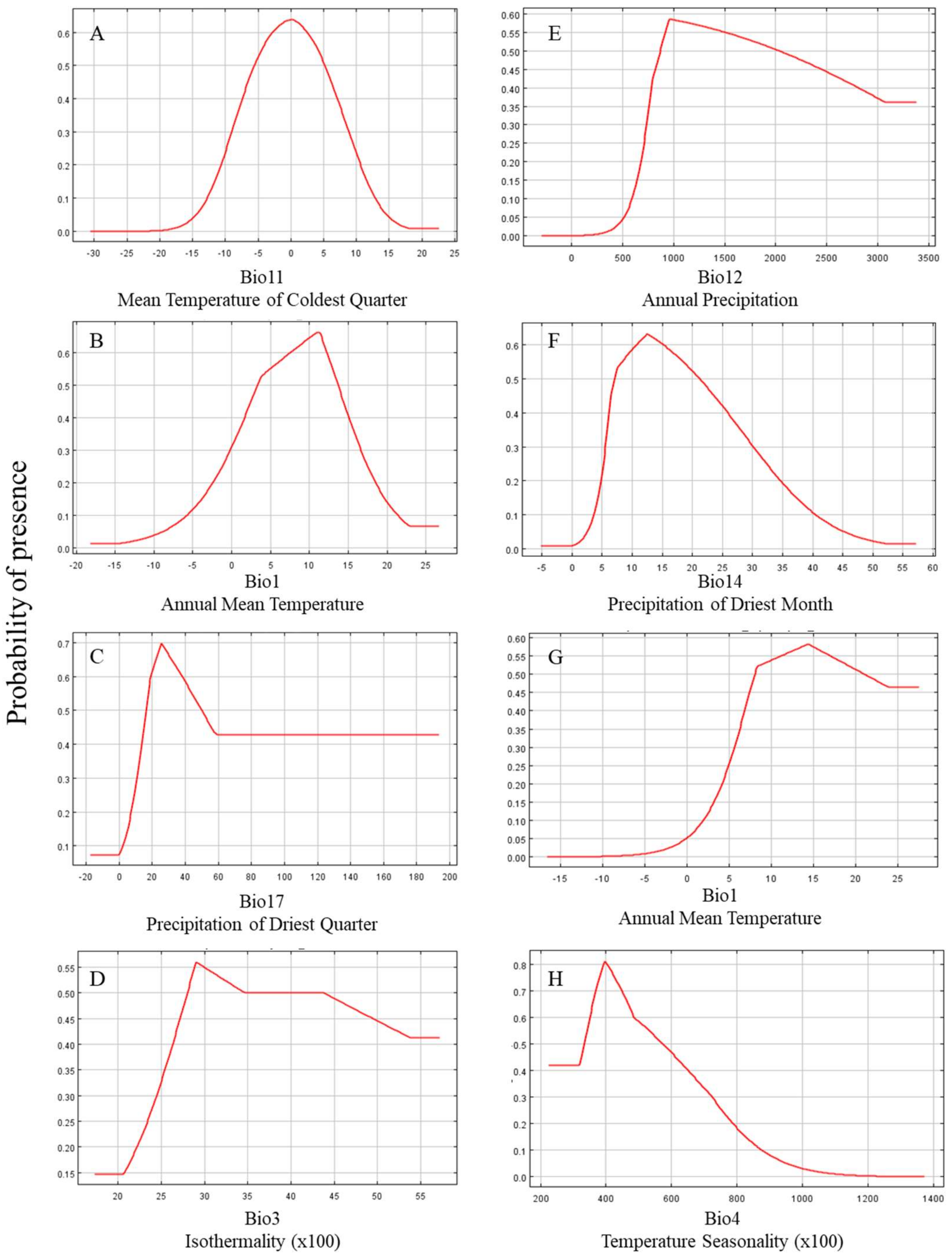
3.2. Important Environmental Variables of Chodsigoa hypsibia and Anourosorex squamipes

The total of the first four environmental factors’ contributions to the MaxEnt model reached 99.2%. We selected the first four factors as the major factors influencing the distribution of C. hypsibia in the recent climate model. They included the mean temperature of the coldest quarter (contributing 47.4%), annual mean temperature (contributing 24.7%), precipitation of the driest quarter (contributing 21.1%) and isothermality (contributing 6%). Annual precipitation (contributing 42.9%), precipitation of the driest month (contributing 28.1%), annual mean temperature (contributing 14.8%) and temperature seasonality (contributing 12.6%) had the greatest contributions to the distribution model for A. squamipes. The total of the first four environmental factors’ contributions reached 98.4% (Table 2).
Using the response curves, we obtained the thresholds (occurrence probability N > 0.5) for the main bioclimatic parameters in the current climate scenario. In C. hypsibia, mean temperature of the coldest quarter (BIO11) ranged from −5 to 5 °C, annual mean temperature from 4 to 14 °C, precipitation of the driest quarter (BIO17) from 20 to 50 mm and isothermality from 28 to 44 °C. Annual precipitation (BIO12) in A. squamipes ranged from 800 to 2500 mm, precipitation of the driest month (BIO14) from 7 to 27 mm, annual mean temperature (BIO1) from 7 to 20 °C and temperature seasonality (BIO4) from 3.5 to 6 °C (Figure 2).

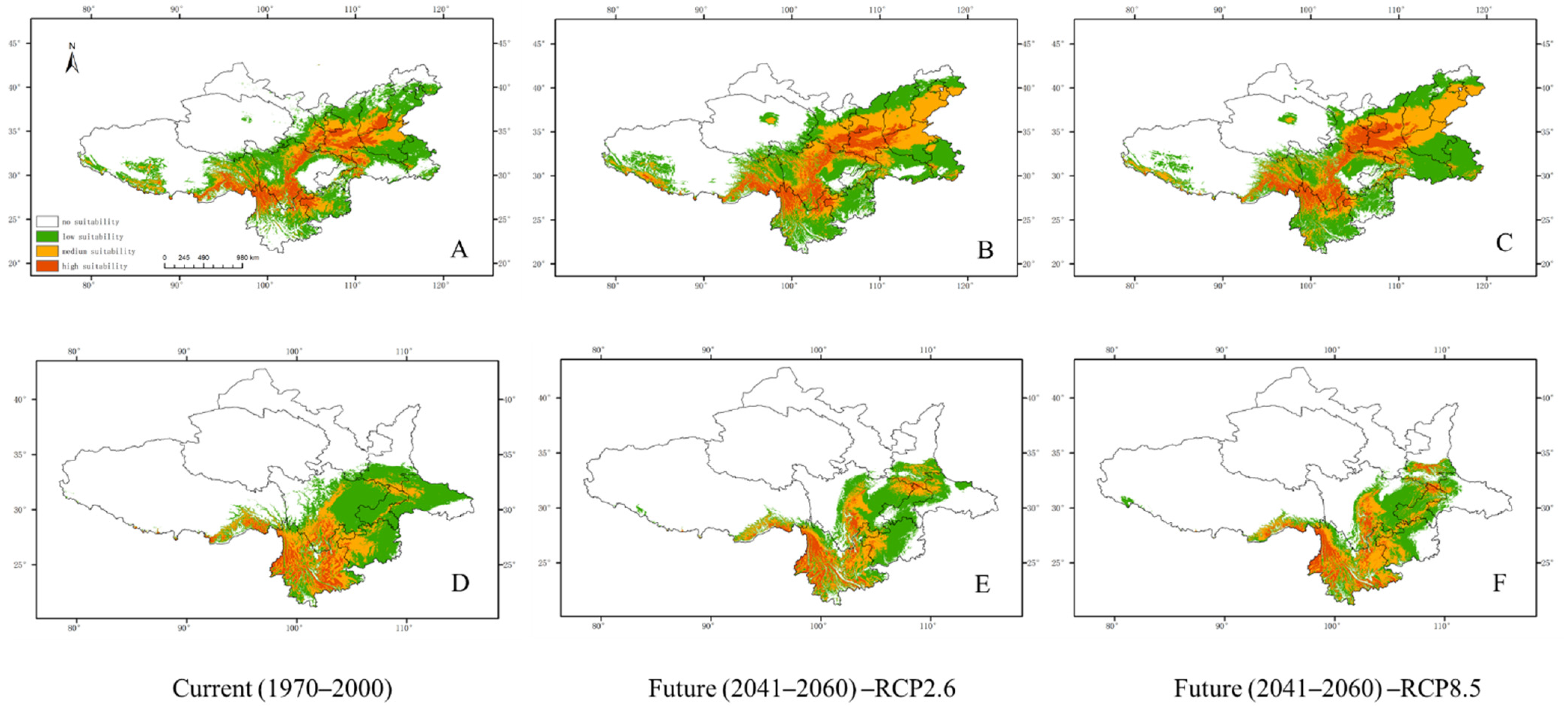
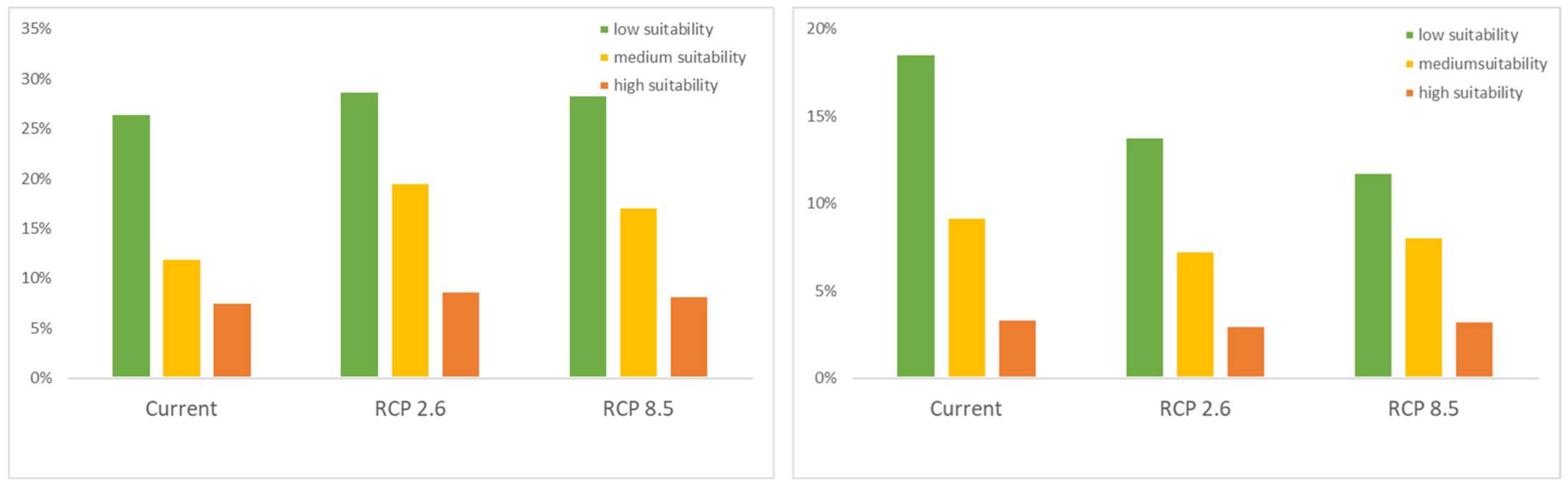
3.3. The Percentage Area of Current and Future Suitable Habitat of C. hypsibia and A. squamipes

The current and future models projected three different suitable areas for C. hypsibia and A. squamipes (Figure 3). The proportion in total areas for the low, medium and high suitability were 26.5%, 12% and 7.6%, respectively, in the current climatic scenario of C. hypsibia. We found a large suitable area in the RCP 2.6 and RCP 8.5 scenarios, with predicted gains in habitat extent. Under RCP2.6, the three suitable areas (low, medium and high) increased to 28.8%, 19.6% and 8.7%, respectively; under RCP8.5, the three suitable areas increased to 28.4%, 17.2% and 8.3%, respectively. For A. squamipes, the proportion in total areas for the low, medium and high suitability were 26.5%, 12% and 7.6% in the current climatic scenario whereas the suitable area under future climatic scenarios deceased. The high suitable area changed little, while the low and medium suitable area decreased to 13.8% and 7.3% under RCP 2.6, respectively, and 11.8% and 8.1% under RCP 8.5, respectively (Figure 4).

4. Discussion

The response of small mammals to climate change has reported different results. A study of 34 species of small mammals in montane California showed that the lower limits of the distribution of high-elevation species moves upward generally, and that temperature change is a better prediction of migration direction than precipitation; low-elevation species had heterogeneous responses, as temperature and precipitation changes could not predict migration direction [31]. Baltensperger and Huettmann [32] predicted the distribution of 17 small mammals in Alaska: climate change is causing species in the cold northern regions to gradually move northward and are facing large areas of habitat loss, while species in the southern regions gradually expanded as they moved to the coast. Studies have shown that the population dynamic of forest voles in the northern Urals have changed significantly from 2003 to 2015. Shrinking forest habitat caused by climatic change may be one of the most important factors affecting the population of small mammals [33]. We performed analysis on the suitable habitat of two shrew species under current and future climate scenarios, providing biological and ecological references and suggestions for the small mammals of China.
A decrease in precipitation of the driest quarter and annual precipitation greatly reduced the occurrence probability of Chodsigoa hypsibia and Anourosorex squamipes, indicating that precipitation is an important constraint to their distribution. Precipitation causes changes in soil moisture, affecting the growth of plants [34]. Shrews are more attracted to moist and dense forests, which are conducive for hiding and foraging due to abundant fallen leaves and food. According to the response curve of annual mean temperature, the suitable temperature of A. squamipes is higher than C. hypsibia; this may be related to the altitude at which they are distributed. Mid- and high-elevation altitudes are suitable for C. hypsibia, but mid- and low-elevation altitudes are suitable for A. squamipes. A striking feature of elevational gradients is the succession of habitats, which is directly related to the climatic variables [35]. Because many insectivore subfamilies prefer warm and humid climates, species distribution patterns are more affected by the humid, warm, and cool climates of middle elevation areas [19]. In addition, the mean temperature of the coldest quarter lower than 0 °C greatly reduced the probability of C. hypsibia presence. Small homothermic animals such as Soricids dissipate heat easily as their weight does not reach the threshold for maintaining constant temperatures [36]. C. hypsibia has significant metabolic expenditures at cold ambient temperatures, as well as poor starvation resistance, due to its smaller body size and higher metabolic rate. Temperature seasonality higher than 6 °C reduced the probability of the presence of A. squamipes. As the reproduction of A. squamipes is affected by external factors such as temperature, areas with severe seasonal temperature fluctuations may limit their distribution.
Under the different scenarios of concentration of greenhouse gas emissions (RCP2.6 and RCP8.5), the percentage of suitable habitat range of A. squamipes decreased compared with the current scenario. Annual precipitation (BIO12) was one of the main influencing factors, with a suitable range between 1200 mm and 2500 mm, which is a decrease compared with the current climatic scenario. In addition, factors related to precipitation had a great influence on A. squamipes, suggesting that precipitation may be the main factor affecting the distribution of A. squamipes. Increasing extreme weather events and heavy precipitation events may further decrease the suitable area of A. squamipes. With global warming, A. squamipes may migrate to high latitudes or high elevations as suitable habitat decreases further [37,38]. Under the future climatic scenario, the percentage of suitable habitat range of C. hypsibia will increase compared with the current scenario due to the increasing intensity of global warming. Under the response curve in the future climatic scenario, both temperature and precipitation (BIO11 and BIO17) affect the suitable areas for C. hypsibia. Warmer temperatures linked to global warming are projected to result in more frequent rainstorms [1], which could lead to some currently unsuitable areas becoming suitable. This might explain the pattern of change shown in the simulated species distribution. In addition, the distributions may have been influenced by ice age conditions in East Asia, especially the LGM (last glacial maximum), which could have led to the retreat of Nectogalini shrews (a higher taxon of Chodsigoa) to Taiwan, Southwest China and even further south in Southwest Asia as refugia, where they have dispersed broadly [39]. After the LGM, a warm and wet climate might have allowed Chodsigoa to spread widely in central and south China [40]. As climate continues to warm, these populations are likely to expand further.
Despite its simplicity and generally high prediction accuracy, the MaxEnt model has several limitations [41]. Firstly, the distribution of species is not only related to external environmental climatic conditions but also to internal physiological and biochemical responses, such as sensitivities to minimum and maximum temperatures at critical times of their life cycle [42]. Species are affected to different extents by inter-species interactions (competition and facilitation), which may drive species distributions [43,44]. Dispersal restrictions can also limit the distribution of a species by preventing it from accessing a suitable habitat [45]. In addition, the modeling approach limits the predictive power to some extent. Previous studies have shown that the MaxEnt model still performs well when the sample size is small. However, it is only in areas where the environment is similar to the populations of species currently maintained, meaning that there is still uncertainty about what we predict [46]. The AUC’s assessment approach may produce exaggerated estimates of niche models, which may require hypothesis testing using the null model, although this approach is currently rarely used in the field [47]. Despite the limitations in the modeling approach, SDMs can be a useful tool for supplementing laboratory and field data to gain a better understanding of species biology and ecology, especially when only limited information is available.

5. Conclusions

In this study, we simulated the distribution of Chodsigoa hypsibia and Anourosorex squamipes using an ecological niche model under two future climate scenarios. The findings demonstrate that different small mammal species respond differently to climate change. The suitability of C. hypsibia showed an expansion under RCP2.6 and RCP8.5, but there was an opposite trend for A. squamipes. The combination of temperature and precipitation could lead to some currently unsuitable areas of C. hypsibia becoming suitable. Distribution contraction of A. squamipes is more affected by precipitation factors. Our study provides biological and ecological references and suggestions for small mammal distribution responses to projected climate change scenarios.

Supplementary Materials

The following supporting information can be downloaded at: https://www.mdpi.com/article/10.3390/d14020087/s1, Table S1: Occurrence records used for MaxEnt Model of Chodsigoa hypsibia and Anourosorex squamipes in China. Table S2: Correlation matrix of variables selected for MaxEnt model of Chodsigoa hypsibia (a) and Anourosorex squamipes (b).

Author Contributions

Z.C., X.J., H.W. and W.H. conceived, designed and planned the study; W.H. performed analyses and led the writing; K.O.O. reviewed drafts of the paper and contributed to the data analyses. All authors have read and agreed to the published version of the manuscript.

Funding

The study was supported by the National Natural Science Foundation of China (No. 31900318), Anhui Provincial Natural Science Foundation (2008085QC106), and the Second Tibetan Plateau Scientific Expedition and Research Program (STEP, No. 2019QZKK0501).

Institutional Review Board Statement

Not applicable.

Data Availability Statement

Not applicable.

Conflicts of Interest

The authors declare no conflict of interest.

References

  1. Hoffmann, A.A.; Sgrò, C.M. Climate change and evolutionary adaptation. Nature 2011, 470, 479–485. [Google Scholar] [CrossRef]
  2. Mohajan, H. Greenhouse Gas Emissions, Global Warming and Climate Change. In Proceedings of the 15th Chittagong Conference on Mathematical Physics, Jamal Nazrul Islam Research Centre for Mathematical and Physical Sciences (JNIRCMPS), Chittagong, Bangladesh, 16 March 2017. [Google Scholar]
  3. Elith, J.; Leathwick, J.R. Species Distribution Models: Ecological Explanation and Prediction Across Space and Time. Annu. Rev. Ecol. Evol. Syst. 2009, 40, 677–697. [Google Scholar] [CrossRef]
  4. Levinsky, I.; Skov, F.; Svenning, J.-C.; Rahbek, C. Potential impacts of climate change on the distributions and diversity patterns of European mammals. Biodivers. Conserv. 2007, 16, 3803–3816. [Google Scholar] [CrossRef]
  5. Ellis, E.C. Anthropogenic transformation of the terrestrial biosphere. Philos. Trans. R. Soc. A Math. Phys. Eng. Sci. 2011, 369, 1010–1035. [Google Scholar] [CrossRef]
  6. Phillips, S.J.; Anderson, R.P.; Schapire, R.E. Maximum entropy modeling of species geographic distributions. Ecol. Model. 2006, 190, 231–259. [Google Scholar] [CrossRef] [Green Version]
  7. Manzoor, S.A.; Griffiths, G.; Obiakara, M.C.; Esparza-Estrada, C.E.; Lukac, M. Evidence of ecological niche shift in Rhododendron ponticum (L.) in Britain: Hybridization as a possible cause of rapid niche expansion. Ecol. Evol. 2020, 10, 2040–2050. [Google Scholar] [CrossRef] [Green Version]
  8. Yan, H.; Feng, L.; Zhao, Y.; Feng, L.; Wu, D.; Zhu, C. Prediction of the spatial distribution of Alternanthera philoxeroides in China based on ArcGIS and MaxEnt. Glob. Ecol. Conserv. 2020, 21, e00856. [Google Scholar] [CrossRef]
  9. Renard, Q.; Pélissier, R.; Ramesh, B.; Kodandapani, N. Environmental susceptibility model for predicting forest fire occurrence in the Western Ghats of India. Int. J. Wildland Fire 2012, 21, 368–379. [Google Scholar] [CrossRef] [Green Version]
  10. Yue, Y.; Zhang, P.; Shang, Y. The potential global distribution and dynamics of wheat under multiple climate change scenarios. Sci. Total Environ. 2019, 688, 1308–1318. [Google Scholar] [CrossRef]
  11. Wan, J.; Qi, G.-j.; Ma, J.; Ren, Y.; Wang, R.; McKirdy, S. Predicting the potential geographic distribution of Bactrocera bryoniae and Bactrocera neohumeralis (Diptera: Tephritidae) in China using MaxEnt ecological niche modeling. J. Integr. Agric. 2020, 19, 2072–2082. [Google Scholar] [CrossRef]
  12. Merow, C.; Silander, J.A.; Warton, D. A comparison of Maxlike and Maxent for modelling species distributions. Methods Ecol. Evol. 2014, 5, 215–225. [Google Scholar] [CrossRef]
  13. Olofsson, P.; Foody, G.M.; Herold, M.; Stehman, S.V.; Woodcock, C.E.; Wulder, M.A. Good practices for estimating area and assessing accuracy of land change. Remote Sens. Environ. 2014, 148, 42–57. [Google Scholar] [CrossRef]
  14. Gilg, O.; Sittler, B.T.; Hanski, I. Climate change and cyclic predator–prey population dynamics in the high Arctic. Glob. Change Biol. 2009, 15, 2634–2652. [Google Scholar] [CrossRef]
  15. McCain, C.M.; Colwell, R.K. Assessing the threat to montane biodiversity from discordant shifts in temperature and precipitation in a changing climate. Ecol. Lett. 2011, 14, 1236–1245. [Google Scholar] [CrossRef]
  16. Brown, C.R.; Hunter, E.M.; Baxter, R.M. Metabolism and thermoregulation in the forest shrew Myosorex varius (Soricidae: Crocidurinae). Comp. Biochem. Physiol. Part A Physiol. 1997, 118, 1285–1290. [Google Scholar] [CrossRef]
  17. Wells, K.; Pfeiffer, M.; Lakim, M.; Linsenmair, K.E. Use of arboreal and terrestrial space by a small mammal community in a tropical rain forest in Borneo, Malaysia. J. Biogeogr. 2004, 31, 641–652. [Google Scholar] [CrossRef]
  18. Umetsu, F.; Metzger, J.; Pardini, R. Importance of estimating matrix quality for modeling species distribution in complex tropical landscapes: A test with Atlantic forest small mammals. Ecography 2008, 31, 359–370. [Google Scholar] [CrossRef]
  19. Andrew, T.S.; Yan, X.; Robert, S.H.; Darrin, L.; John, M.; Don, E.W.; Wozencraft, W.C. A Guide to the Mammals of China; Princeton University Press: Princeton, NJ, USA, 2010. [Google Scholar]
  20. He, K.; Hu, N.Q.; Chen, X.; Li, J.T.; Jiang, X.L. Interglacial refugia preserved high genetic diversity of the Chinese mole shrew in the mountains of southwest China. Heredity 2016, 116, 23–32. [Google Scholar] [CrossRef] [Green Version]
  21. Chen, Z.-Z.; He, K.; Huang, C.; Wan, T.; Lin, L.-K.; Liu, S.-Y.; Jiang, X.-L. Integrative systematic analyses of the genus Chodsigoa (Mammalia: Eulipotyphla: Soricidae), with descriptions of new species. Zool. J. Linn. Soc. 2017, 180, 694–713. [Google Scholar] [CrossRef]
  22. Hijmans, R.J.; Cameron, S.E.; Parra, J.L.; Jones, P.G.; Jarvis, A. Very high resolution interpolated climate surfaces for global land areas. Int. J. Climatol. 2005, 25, 1965–1978. [Google Scholar] [CrossRef]
  23. Ashoori, A.; Kafash, A.; Varasteh Moradi, H.; Yousefi, M.; Kamyab, H.; Behdarvand, N.; Mohammadi, S. Habitat modeling of the common pheasant Phasianus colchicus (Galliformes: Phasianidae) in a highly modified landscape: Application of species distribution models in the study of a poorly documented bird in Iran. Eur. Zool. J. 2018, 85, 372–380. [Google Scholar] [CrossRef] [Green Version]
  24. Meinshausen, M.; Smith, S.J.; Calvin, K.; Daniel, J.S.; Kainuma, M.L.T.; Lamarque, J.F.; Matsumoto, K.; Montzka, S.A.; Raper, S.C.B.; Riahi, K.; et al. The RCP greenhouse gas concentrations and their extensions from 1765 to 2300. Clim. Change 2011, 109, 213–241. [Google Scholar] [CrossRef] [Green Version]
  25. Farashi, A.; Erfani, M. Modeling of habitat suitability of Asiatic black bear (Ursus thibetanus gedrosianus) in Iran in future. Acta Ecol. Sin. 2018, 38, 9–14. [Google Scholar] [CrossRef]
  26. Liang, T.; Feng, Q.; Yu, H.; Huang, X.; Lin, H.; An, S.; Ren, J. Dynamics of natural vegetation on the Tibetan Plateau from past to future using a comprehensive and sequential classification system and remote sensing data. Grassl. Sci. 2012, 58, 208–220. [Google Scholar] [CrossRef]
  27. Mohammadi, S.; Ebrahimi, E.; Shahriari Moghadam, M.; Bosso, L. Modelling current and future potential distributions of two desert jerboas under climate change in Iran. Ecol. Inform. 2019, 52, 7–13. [Google Scholar] [CrossRef]
  28. Bosso, L.; Smeraldo, S.; Rapuzzi, P.; Sama, G.; Garonna, A.P.; Russo, D. Nature protection areas of Europe are insufficient to preserve the threatened beetleRosalia alpine (Coleoptera: Cerambycidae): Evidence from species distribution models and conservation gap analysis. Ecol. Entomol. 2018, 43, 192–203. [Google Scholar] [CrossRef]
  29. Phillips, S.J.; Dudík, M. Modeling of species distributions with Maxent: New extensions and a comprehensive evaluation. Ecography 2008, 31, 161–175. [Google Scholar] [CrossRef]
  30. Phillips, S.J.; Anderson, R.P.; Dudík, M.; Schapire, R.E.; Blair, M.E. Opening the black box: An open-source release of Maxent. Ecography 2017, 40, 887–893. [Google Scholar] [CrossRef]
  31. Rowe, K.C.; Rowe, K.M.; Tingley, M.W.; Koo, M.S.; Patton, J.L.; Conroy, C.; Perrine, J.D.; Beissinger, S.R.; Moritz, C. Spatially heterogeneous impact of climate change on small mammals of montane California. Proc. R. Soc. B Biol. Sci. 2015, 282, 20141857. [Google Scholar] [CrossRef] [Green Version]
  32. Baltensperger, A.P.; Huettmann, F. Predicted Shifts in Small Mammal Distributions and Biodiversity in the Altered Future Environment of Alaska: An Open Access Data and Machine Learning Perspective. PLoS ONE 2015, 10, e0132054. [Google Scholar] [CrossRef]
  33. Bobretsov, A.V.; Lukyanova, L.E.; Bykhovets, N.M.; Petrov, A.N. Impact of climate change on population dynamics of forest voles (Myodes) in northern Pre-Urals: The role of landscape effects. Contemp. Probl. Ecol. 2017, 10, 215–223. [Google Scholar] [CrossRef]
  34. Harris, R.B. A Guide to the Mammals of China by A. T. Smith and Y. Xie (eds.). J. Mammal. 2009, 90, 520–521. [Google Scholar] [CrossRef]
  35. McCain, C.M. Elevational Gradients in Diversity of Small Mammals. Ecology 2005, 86, 366–372. [Google Scholar] [CrossRef]
  36. Pearson, O.P. Metabolism of Small Mammals, With Remarks on the Lower Limit of Mammalian Size. Science 1948, 108, 44. [Google Scholar] [CrossRef]
  37. Parmesan, C.; Yohe, G. A globally coherent fingerprint of climate change impacts across natural systems. Nature 2003, 421, 37–42. [Google Scholar] [CrossRef]
  38. Bertrand, R.; Lenoir, J.; Piedallu, C.; Riofrío-Dillon, G.; de Ruffray, P.; Vidal, C.; Pierrat, J.-C.; Gégout, J.-C. Changes in plant community composition lag behind climate warming in lowland forests. Nature 2011, 479, 517–520. [Google Scholar] [CrossRef]
  39. Hutterer, R. Order Soricomorpha. In Mammal Species of the World: A Taxonomic and Geographic Reference, 3rd ed.; Wilson, D.E., Reeder, D.M., Eds.; Johns Hopkins University Press: Baltimore, MD, USA, 2005. [Google Scholar]
  40. He, K.; Li, Y.J.; Brandley, M.C.; Lin, L.K.; Wang, Y.X.; Zhang, Y.P.; Jiang, X.L. A multi-locus phylogeny of Nectogalini shrews and influences of the paleoclimate on speciation and evolution. Mol. Phylogenetics Evol. 2010, 56, 734–746. [Google Scholar] [CrossRef]
  41. Xu, D.; Zhuo, Z.; Wang, R.; Ye, M.; Pu, B. Modeling the distribution of Zanthoxylum armatum in China with MaxEnt modeling. Glob. Ecol. Conserv. 2019, 19, e00691. [Google Scholar] [CrossRef]
  42. Chen, I.-C.; Hill, J.K.; Ohlemüller, R.; Roy, D.B.; Thomas, C.D. Rapid Range Shifts of Species Associated with High Levels of Climate Warming. Science 2011, 333, 1024–1026. [Google Scholar] [CrossRef]
  43. Lortie, C.J.; Brooker, R.W.; Choler, P.; Kikvidze, Z.; Michalet, R.; Pugnaire, F.I.; Callaway, R.M. Rethinking plant community theory. Oikos 2004, 107, 433–438. [Google Scholar] [CrossRef]
  44. Warren, M.S.; Hill, J.K.; Thomas, J.A.; Asher, J.; Fox, R.; Huntley, B.; Roy, D.B.; Telfer, M.G.; Jeffcoate, S.; Harding, P.; et al. Rapid responses of British butterflies to opposing forces of climate and habitat change. Nature 2001, 414, 65–69. [Google Scholar] [CrossRef] [Green Version]
  45. Vellend, M.; Verheyen, K.; Flinn, K.M.; Jacquemyn, H.; Kolb, A.; Van Calster, H.; Peterken, G.; Graae, B.J.; Bellemare, J.; Honnay, O.; et al. Homogenization of forest plant communities and weakening of species? Environment relationships via agricultural land use. J. Ecol. 2007, 95, 565–573. [Google Scholar] [CrossRef]
  46. Pearson, R.G.; Raxworthy, C.J.; Nakamura, M.; Townsend Peterson, A. Predicting species distributions from small numbers of occurrence records: A test case using cryptic geckos in Madagascar. J. Biogeogr. 2006, 34, 102–117. [Google Scholar] [CrossRef]
  47. Bohl, C.L.; Kass, J.M.; Anderson, R.P. A new null model approach to quantify performance and significance for ecological niche models of species distributions. J. Biogeogr. 2019, 46, 1101–1111. [Google Scholar] [CrossRef]
Figure 1. Distribution records of Chodsigoa hypsibia and Anourosorex squamipes in China.
Diversity 14 00087 g001
Figure 2. Response curves for the first three important environmental predictors in the species distribution model for Chodsigoa hypsibia (AD) and Anourosorex squamipes (EH) in the current climate scenario.
Diversity 14 00087 g002
Figure 3. Maps showing the MaxEnt-modelled current and future (2050: RCP2.6 and RCP8.5) distributions of C. hypsibia (AC) and A. squamipes (DF).
Diversity 14 00087 g003
Figure 4. Percentage area of Chodsigoa hypsibia (left) and Anourosorex squamipes (right) for three different suitable distributions under current and future climate scenarios (RCP2.6 and RCP8.5).
Diversity 14 00087 g004
Table 1. List of environmental variables considered in this study.
CodeBioclimatic Variables
BIO 1Annual mean temperature (°C)
BIO 2Mean diurnal range (Mean of monthly (max temp–min temp)) (°C)
BIO 3Isothermality ((BIO2/BIO7) *100) (°C)
BIO 4Temperature seasonality (standard deviation *100) (°C)
BIO 5Maximum temperature of warmest month (°C)
BIO 6Minimum temperature of coldest month (°C)
BIO 7Temperature annual range (BIO5–BIO6) (°C)
BIO 8Mean temperature of wettest quarter (°C)
BIO 9Mean temperature of driest quarter (°C)
BIO 10Mean temperature of warmest quarter (°C)
BIO 11Mean temperature of coldest quarter (°C)
BIO 12Annual precipitation (mm)
BIO 13Precipitation of wettest month (mm)
BIO 14Precipitation of driest month (mm)
BIO 15Precipitation seasonality (standard deviation *100) (°C)
BIO 16Precipitation of wettest quarter (mm)
BIO 17Precipitation of driest quarter (mm)
BIO 18Precipitation of warmest quarter (mm)
BIO 19
ELEV
Precipitation of coldest quarter (mm)
Elevation (m)
Table 2. Percent contribution of the first four variables used to model the current and future potential distribution of Chodsigoa hypsibia and Anourosorex squamipes in China.
SpeciesModelAUCPercent Contribution of the First Four Variables
C. hypsibiaCurrent (1970–2000)0.90BIO11(47.4%), BIO1(24.7%), BIO17(21.1%), BIO3(6%)
Future (2041–2060)-RCP2.60.91BIO17(41.7%), BIO11(36.3%), BIO1(16.8%), BIO14(4.7%)
Future (2041–2060)-RCP8.50.92BIO17(41.6%), BIO11(32.5%), BIO1(18.3%), BIO19(3.2%)
A. squamipesCurrent (1970–2000)0.91BIO12(42.9%), BIO14(28.1%), BIO1(14.8%), BIO4(12.6%)
Future (2041–2060)-RCP2.60.92BIO12(29.6%), BIO17(22.8%), BIO14(20.1%), BIO4(13.5%)
Future (2041–2060)-RCP8.50.93BIO14(58.8%), BIO12(25.4%), BIO2(7.9%), BIO1(5.8%)
Publisher’s Note: MDPI stays neutral with regard to jurisdictional claims in published maps and institutional affiliations.

