Article

Genetic Divergence between Two Sympatric Ecotypes of Phalaenopsis pulcherrima on Hainan Island

1
Key Laboratory of Genetics and Germplasm Innovation of Tropical Special Forest Trees and Ornamental Plants, Ministry of Education, Hainan University, Haikou 570228, China
2
College of Forestry, Hainan University, Haikou 570228, China
3
College of Landscape Architecture, Fujian Agricultural and Forestry University, Fuzhou 350002, China
*
Authors to whom correspondence should be addressed.
Diversity 2021, 13(9), 446; https://doi.org/10.3390/d13090446
Submission received: 14 August 2021 / Revised: 9 September 2021 / Accepted: 14 September 2021 / Published: 17 September 2021
(This article belongs to the Special Issue Conservation Genetics and Biogeography of Seed Plant Species)

Abstract

:
Ecotypes are the result of ecological differentiation at the early stages of speciation. Adaptation to soil conditions offers arguably the best examples of local adaptation in plants. Two sympatric ecotypes, with either a red or green abaxial leaf surface, were found without clear geographical isolation in Phalaenopsis pulcherrima, a Southeast Asia endemic and endangered orchid. The soil of the red leaf ecotype has a higher water content and nutrient content than the green ecotype. What is the genetic structure of the two ecotypes? Is there complete or partial reproductive isolation between the two ecotypes? In this work, leaf reflection of the two ecotypes in P. pulcherrima were compared, to illustrate their difference in leaf color. The genetic differentiation between two ecotypes was examined, using ISSR and SRAP markers to determine the genetic structure of the populations. Our results showed that the green ecotype had reflectance spectrum peaks at 530 nm and 620 nm, while in the red ecotype, the peak at 530 nm was absent. A total of 165 ISSR and SRAP loci showed a high level of genetic diversity within the green ecotype, and analyses of the population structure revealed two genetic clusters that corresponded to the red and green ecotypes. The percentage of variation between the two ecotypes (24.55%) was greater than the percentage of variation among the populations (16.54%)—indicating partial reproductive isolation, high genetic differentiation, and that ecological differentiation has been more important than geographical barriers among populations within ecotypes. Most pairwise FST values between the populations within either ecotype on Hainan Island were less than 0.15; however, the FST between both the Thai and Malaysian populations and the Hainan Island population was greater than 0.25, due to South China sea isolation. Ecotypic differentiation is an important part of speciation; therefore, we must take into account the axes along which lineages sort, when formulating protection strategies.

1. Introduction

Ecotypes refer to groups of individuals within a species, with distinct phenotypic and genetic variations [1,2]. Typically, ecotypes are geographically well separated, but sometimes ecotypes co-exist at the local scale [3,4]. It is widely recognized that ecotypes are the result of ecological differentiation at the early stages of speciation [5,6]. This early stage is often characterized by the formation of partial reproductive isolation [7,8,9,10,11].
Adaptation to soil conditions (edaphic adaptation) offers a classic example of local adaptation in plants [12,13]. Soil attributes, including water content, nutrient status, and toxicity, provide especially rich conditions for divergent natural selection, resulting in divergent morphology, phenology, and, more generally, life history [2,14,15]. Among them, divergence in flowering time is a common cause of reproductive isolation. Inland and coastal ecotypes of the yellow monkeyflower Mimulus guttatus represent an excellent model that is driven by soil water availability [16,17,18,19,20,21,22,23,24]. The inland ecotype has an earlier-flowering, annual life history to escape summer drought conditions, while the coastal ecotype—which receives coastal summer fog and cool temperatures—has maintained a perennial life history that is adapted to year-round soil water availability [16,17,18,19,20,21,22,23,24]. The staggering of the flowering period resulted in the reproductive isolation of the two ecotypes [25]. Ecotypes can emerge at very small spatial scales. For example, Solidago virgaurea ecotypes on serpentine and non-serpentine soils only occur tens of meters apart [12,26,27]. Solidago virgaurea is a perennial and outcrossing herbaceous plant species that is distributed on Hokkaido Island of Japan. The serpentine ecotype is distributed in an open and dry serpentinite area, where the soil is dry and poor, while the non-serpentinite ecotype is distributed in a shaded and mesic non-serpentinite area, where the soil is moist and fertile. As an adaptation to soil conditions, serpentine populations completed flowering by midsummer, versus non-serpentine populations in late summer, which resulted in the reproductive isolation [27]. Ecotypic differentiation can gradually form species over time. For example, sympatric speciation of the palm Howea (Arecaceae) on Lord Howe Island has been traced to a distinct difference in flowering, arising as a physiological response to volcanic and calcarenite substrates that began 1.92 ± 0.53 Myr ago, or less than 1 Myr ago [28]. Toxic soil factors do not typically alter flowering phenology, but heavy metals have been shown to promote rapid population differentiation [29,30,31,32].
The distribution of genetic variation in neutral genetic markers can inform us about patterns of gene flow, population history, and reproductive system, which all influence local adaptation [27]. Molecular markers (e.g., allozymes, amplified fragment length polymorphisms, and microsatellites) often represent neutral genetic variation within and among populations that do not necessarily correspond to adaptive traits [33]. Nevertheless, molecular markers are very useful for detecting population genetic divergence that can indicate ecotypic or epitypic variation [34]. For example, molecular analyses have detected strong population differentiation in North American grasses, suggesting low levels of gene flow and potential ecotypic (or epitypic) divergence among populations [35]. Such marker-based predictions are best combined with field studies to confirm that genetic differentiation reflects adaptive or epistatic variation.
Phalaenopsis pulcherrima is a perennial, self-sterile, predominantly outcrossing orchid, endemic to Southeast Asia, including Hainan Island [36]. It is classified as critically endangered by the Chinese red list (2015). Phalaenopsis pulcherrima is pollinated by bees, mainly by Amegilla zonata and Nomia punctulata, and pollen and seed dispersal distances can reach tens or even hundreds of meters [37]. P. pulcherrima grow on the rocks and soils of the mountains, which are usually shallow, with easily broken rocks that produce dry and exposed environments. Its two ecotypes are characterized by either red or green abaxial leaf surfaces [38]. While the two ecotypes are sympatric at the local scale, they are typically found growing on different substrates. The soil of the red leaf ecotype has higher water and nutrient contents (i.e., available P and K, total P, and exchangeable Ca2+ and Mg2+), and vice versa for the green ecotype [39]. Populations of both the ecotypes, distributed in patches that are 10–30 m apart, exist at distances that are small enough for pollinators and seeds to move between the ecotypes. However, there is a significant boundary between the two ecotypes. So, we hypothesize that the two ecotypes have become entirely or partially reproductively isolated.
In this work, we compare the leaf reflection measurements of the two P. pulcherrima ecotypes, to illustrate their morphological differences. We use molecular markers to assess the genetic structure and degree of reproductive isolation of the two ecotypes, and place it in an evolutionary context. This research can lay the foundation for the further research of the reproductive isolation mechanism, and will be helpful to devise a conservation strategy for this endangered species.

2. Materials and Methods

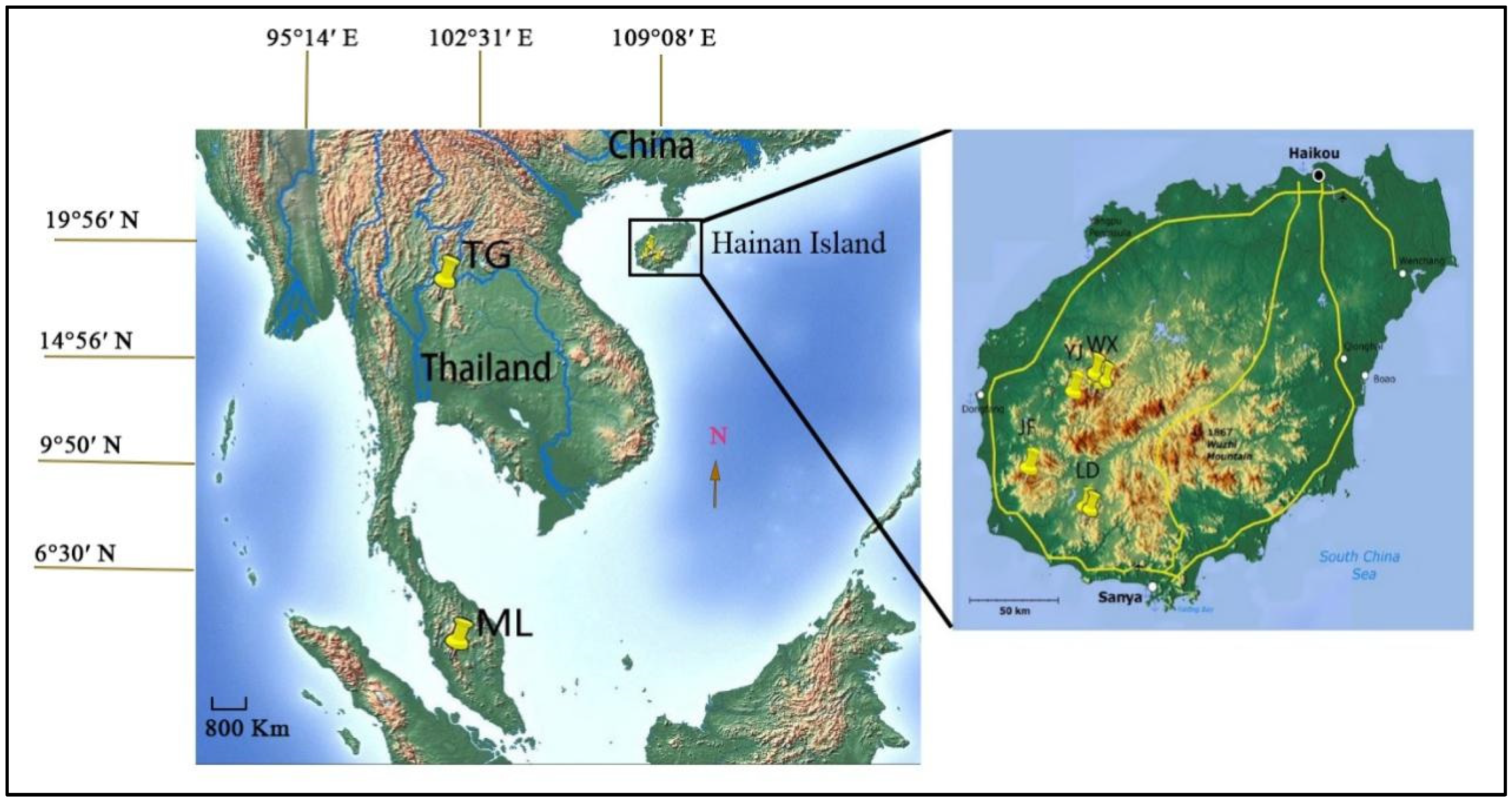
2.1. Population Sampling

Through field surveys, we found a total of 7 populations on Hainan Island that were distributed on 7 mountains (3 in Wangxia, 1 in Yajia, 1 in Jianfeng, and 2 in Ledong) (Figure 1 and Table 1). We sampled these 7 populations, along with 1 population in Thailand and 1 population in Malaysia as outgroups, according to population size and the number of red and green individuals in the population.

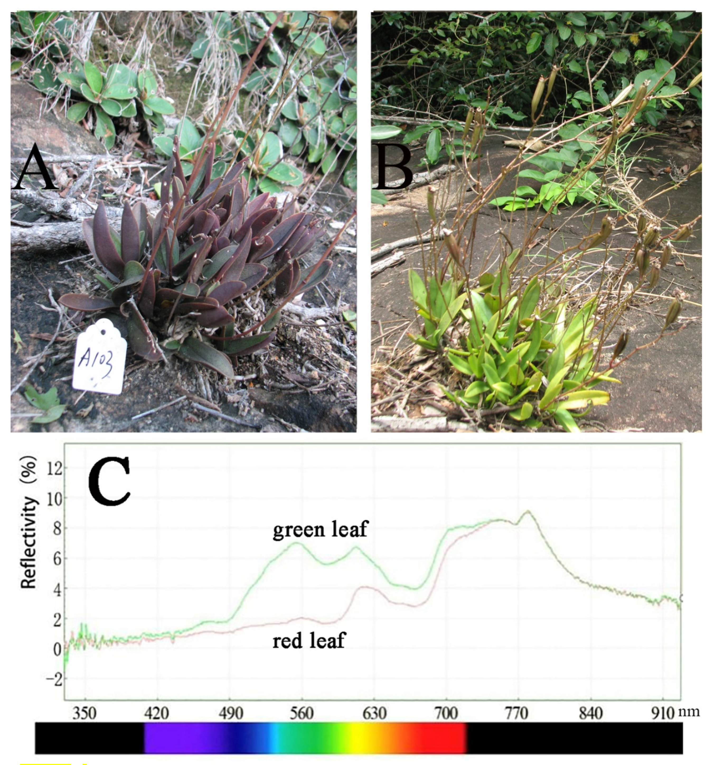
2.2. Leaf Color Reflectance

To assess the light reflection patterns of leaves at different wavelengths, we used an S2000 miniature fiber optic spectrometer with a PX-2 pulsed xenon lamp (Ocean Optics, Dunedin, FL, USA) indoors. All measurements were carried out over the range 350–850 nm using 0.38 nm increments.

2.3. Molecular Markers

2.3.1. DNA Extraction

DNA was extracted using a slightly modified method of Doyle and Doyle [40]; we raised the percentage of PVP in the extraction buffer to 3% for more effective removal of excess polyphenols, and added an additional washing step using 70% cold ethanol before DNA pellets were dried and dissolved in Tris-EDTA buffer. Quantity and quality of extracted DNA was determined in 1% agarose gels buffered with 1 × TAE.

2.3.2. ISSR–PCR Amplification

We used the amplification assay developed by Zietkiewicz et al. [41] to generate inter-simple sequence repeat (ISSR) data. We screened 12 primers (Table 2) from 100 universal primers developed by Biotechnology Laboratory, University of British Columbia, Canada. The reaction mixture for ISSR amplification assay had a total volume of 20 μL, which contained 25 ng genomic DNA, 0.33 mM dNTPs, 1.6 mM MgCl2, 1.5U Taq polymerase, and 0.6 μM primer. The amplification was carried out with an initial 6 min denaturation at 94 °C; 32 cycles of amplification (30 s at 94 °C, annealing 45 s, 90 s at 72 °C); a final extension step for 7 min at 72 °C. The PCR products of each sample, along with a 2 kb DNA ladder, were fractionated on 1.6% agarose gel for 1.5 h at 80 V. The fractionated amplified genomic DNA bands were visualized on UV transilluminator and photographed with a Kodak® digital camera (Kodak, Rochester, NY, USA).

2.3.3. SRAP–PCR Amplification

We screened and used 12 pairs of sequence-related amplified polymorphism (SRAP) primers (Table 2) from 340 combinations of 17 forward and 20 reverse primers. The protocol for SRAP analysis was based on Li and Quiros [42], with modifications. PCR was performed in a total volume of 25 μL containing approximately 40 ng genomic DNA, 0.15 mM dNTPs, 3 mM MgCl2, 0.2 mM of each primer, 1U Taq DNA polymerase using an EDC-810 gene amplification instrument with the following reaction: 6 min of initial denaturation at 94 °C, recycles of five steps of 1 min of denaturation at 94 °C, 1 min of annealing at 35 °C, 1 min of elongation at 72 °C, 33 cycles of 94 °C for 1 min, 50 °C for 1 min, and 72 °C for 1 min, followed by a final extension of 7 min at 72 °C. PCR products were mixed with 10 μL formamide loading buffer (95% formamide and 20 mM EDTA (pH 8.0), Xylene cyanol and Bromophenol blue) and analyzed on 8% non-denaturing polyacrylamide gels in 1 × TBE buffer, with a 200-bp DNA ladder as a size marker. PCR products were visualized by silver staining [43].

2.4. Data Analysis

We used the average measured reflectivity from all individuals of each ecotype to represent the light reflection patterns of the two ecotypes.
Reproducible and consistent ISSR and SRAP fragments were scored as present (1) or absent (0) for all samples, and a binary qualitative data matrix was constructed. Basic estimates of genetic diversity were calculated using POPGENE version 1.32 [44]. Observed number of alleles (na), effective number of alleles (ne), Nei’s gene diversity index (h), Shannon index (I), and principal co-ordinates analysis (PCoA) plots were obtained in GenAlEx 6.41 [45].
Ancestry and clustering analyses were performed in STRUCTURE 2.3.4 [46,47,48] using an “admixture” model with correlated allele frequencies, 1,000,000 iterations after a burn-in of 200,000 iterations, and cluster (K) values ranging from 1 to 10 clusters, with three replicate runs per K. The optimal value of K was determined using ΔK according to the Structure Harvester software [49]. STRUCTURE results obtained using the optimal K value were plotted on the CLUMPAK server [50].
Hierarchical locus-by-locus analyses of molecular variation (AMOVA) were used to evaluate the relative level of genetic variations among groups (FCT), populations within groups (FSC), and individuals within populations (FST); pairwise FST among populations and the significance of each value were tested using Arlequin ver. 3.5 [51,52]. Gene flow (Nm) between populations was estimated from F-statistics with the formula Nm = (1 − FST)/(4FST) [53].
Population- and individual-based cluster analysis was performed using NTSYS-pc software by un-weighted pair group method with arithmetic averages (UPGMA) method.

3. Results

3.1. Leaf Color Reflectance

The two ecotypes showed differences in leaf color. The red ecotype had dark-red leaves on the whole plant, while the green ecotype had light-yellow–green leaves (Figure 2A,B). The green ecotype showed peaks in the reflectance spectrum at 530 nm and 620 nm, while the peak of the red ecotype at 530 nm was absent (Figure 2C).

3.2. Genetic Diversity

We obtained a total of 165 ISSR and SRAP markers (Table 3); 164 loci were polymorphic in the green ecotype, 158 loci in the red ecotype. Nei’s gene diversity (h) and Shannon’s information index (I) were higher in the green ecotype, showing that the green ecotype had a higher genetic diversity (Table 3).

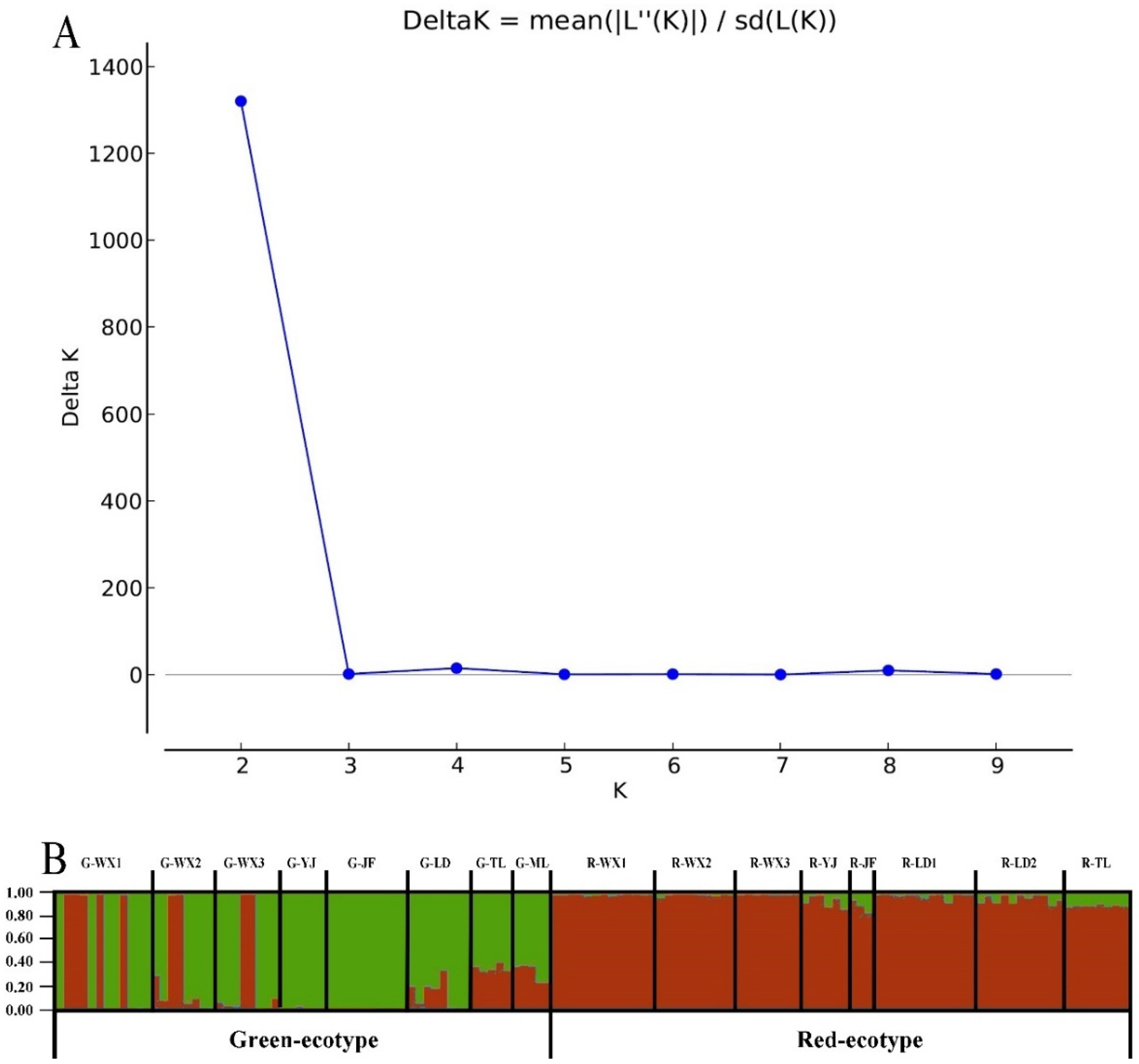
3.3. Inferred Genetic Groups

STRUCTURE analysis showed an obvious peak at K = 2 (Figure 3A), indicating that individuals could best be described by two genetic groups that mostly corresponded to the expected ecotypes, although nine green ecotype individuals (five in WX1, two in WX2, and two in WX3) were classified into the red genetic group (Figure 3B). The assignment probabilities (Q values) of the red ecotype individuals were higher than the green ecotype individuals. The red ecotype individuals had almost 100% red ecotype alleles, while the green ecotype individuals had slightly more varied ancestry, with individuals in the TL and ML populations having about 70% green ecotype alleles (Figure 3B).

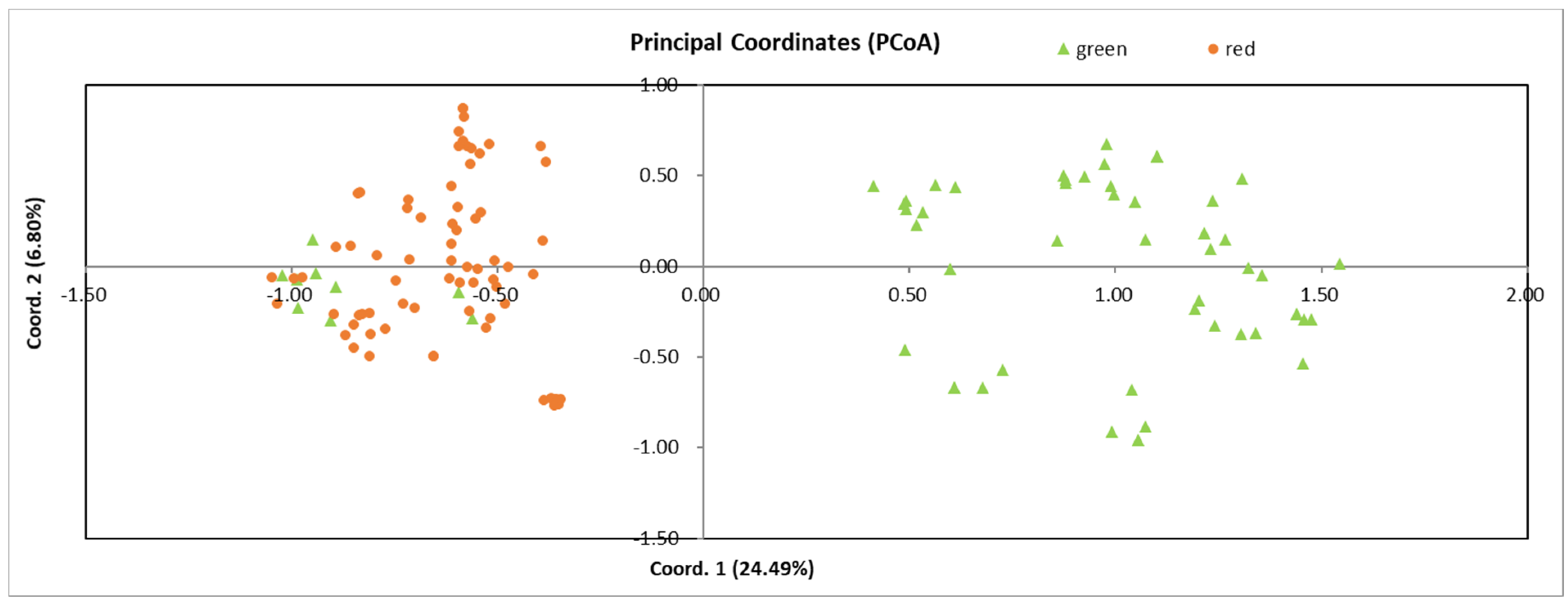
3.4. Genetic Similarity among Individuals

The first two axes of the PCoA explained 31.29% of the total observed variation, with the first two axes explaining 24.49% of and 6.80% of the total variation. The PCoA results showed that the two ecotypes formed mostly distinct clusters, although nine green individuals were clustered more closely to the red ecotype individuals (Figure 4).

3.5. Proportion of Genetic Variance

The AMOVA analyses revealed that most of the genetic variation (58.92%, FST = 0.411, p < 0.001) was distributed among individuals within populations. The percentage of variation between the ecotypes (24.55%, FCT = 0.245, p < 0.001) was larger than that among populations within the ecotypes (16.54%, FSC = 0.219, p < 0.001), indicating that the effect of ecotypes was greater than that of geographical distance (Table 4).

3.6. Genetic Differentiation and Gene Flow among Populations

Most pairwise FST values we measured were significant at the 5% nominal level (Table 5).
It is generally assumed that FST < 0.05 corresponds to no genetic differentiation, 0.05 < FST < 0.15 means moderate genetic differentiation, 0.15 < FST < 0.25 implies high genetic differentiation, and FST > 0.25 implies very high genetic differentiation [54].
In the green ecotype, the FST values among the WX populations (WX1, WX2, WX3) were less than 0.05 (Nm > 4.75). The FST values between the WX populations and YJ were between 0.05 and 0.15 (1.42 < Nm < 4.75). Most of the FST values between the WX populations, and JF, LD, TL, and ML were between 0.15 and 0.25 (0.75 < Nm < 1.42). Most of the FST values among TL, ML, and other populations were greater than 0.25 (Nm < 0.75).
In the red ecotype, most the FST values among WX, YJ, JF, and LD2 were less than 0.15 (Nm > 1.42). Most of the FST values between LD1 and other populations were between 0.15 and 0.25 (0.75 < Nm < 1.42). The FST values between TL and other populations were greater than 0.25 (Nm < 0.75).
Most the FST values between the green and red ecotype populations were greater than 0.25 (Nm < 0.75), indicating very high genetic differentiation. These results show limited gene flow between ecotypes and a gradual decrease in gene flow between populations with the increase in geographic distance.

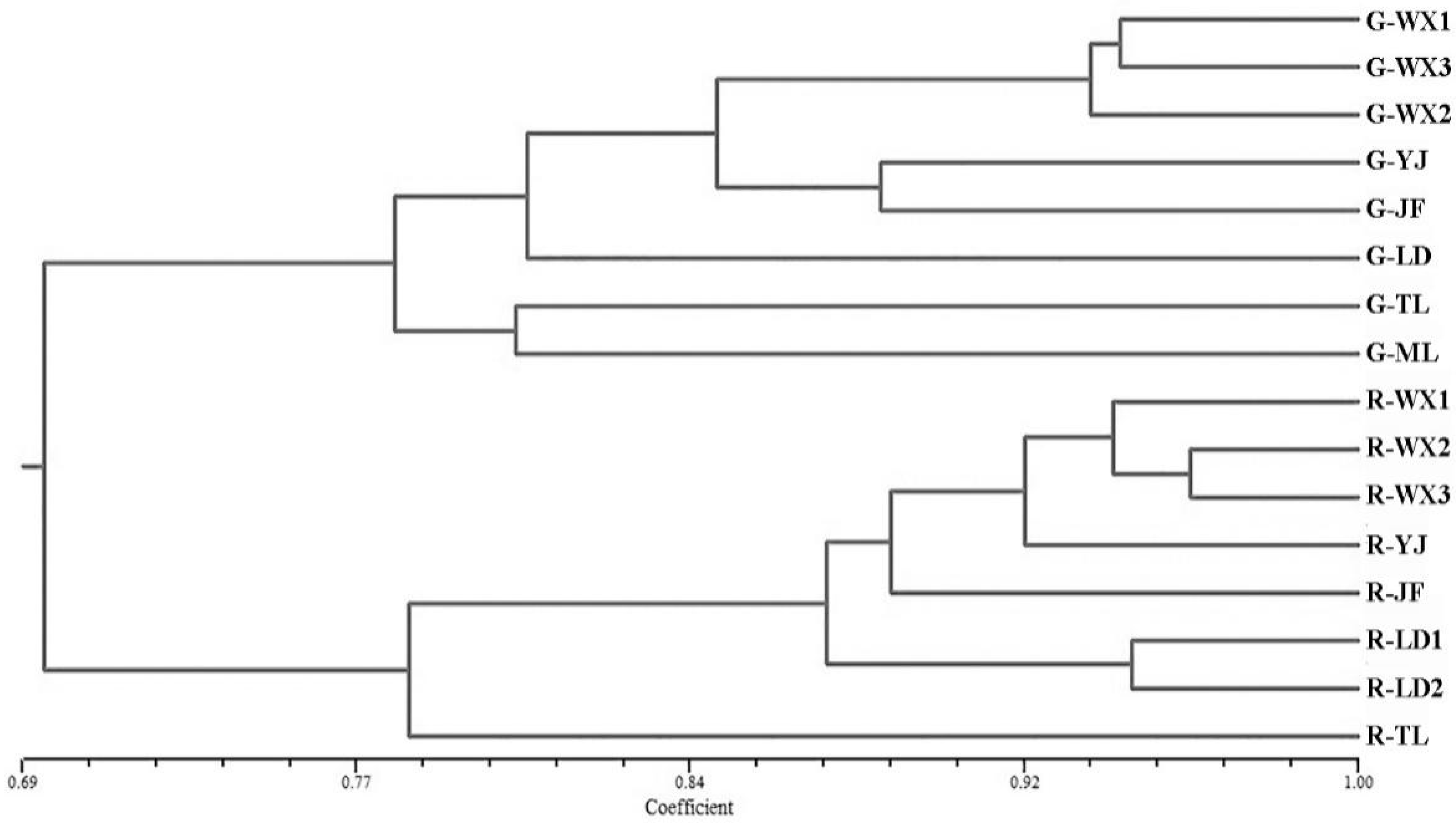
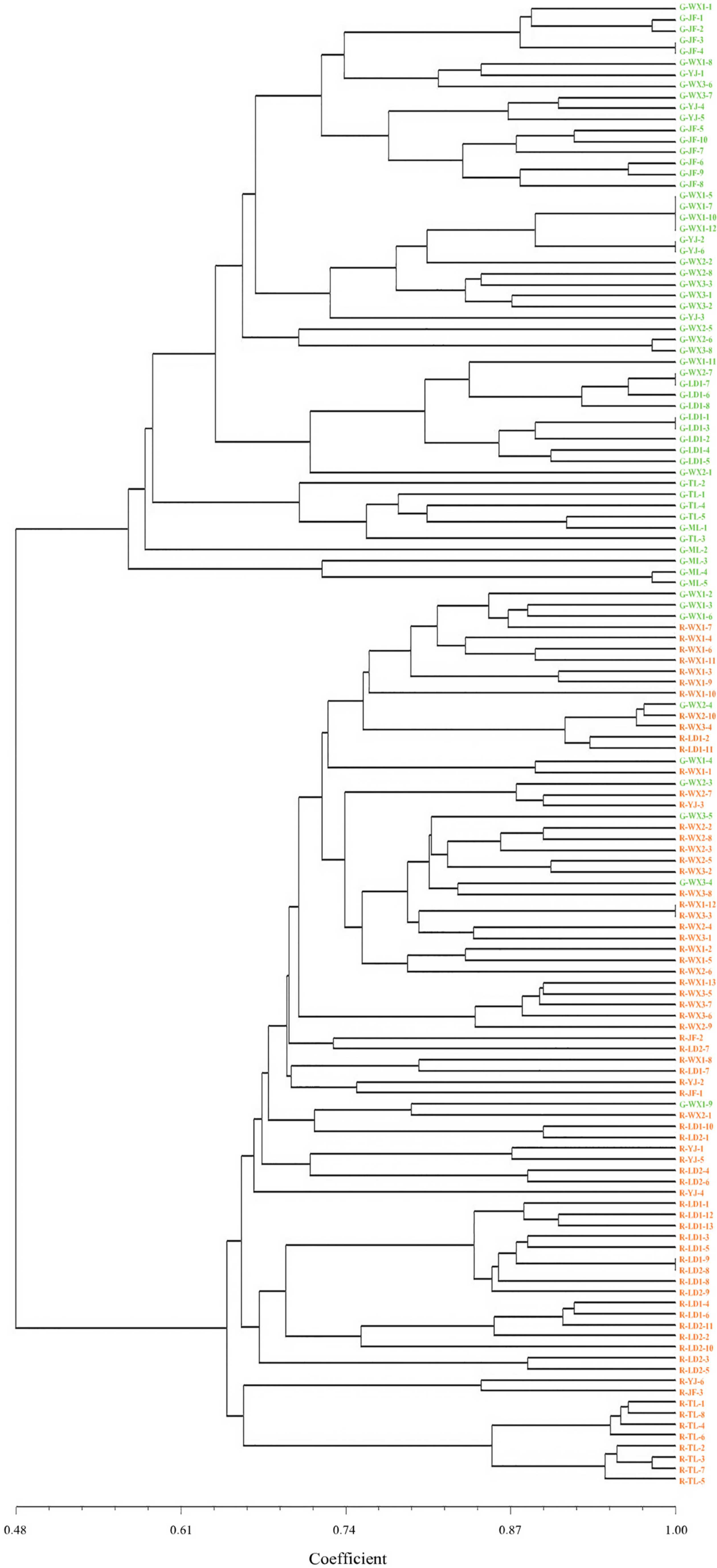
3.7. Genetic Relationships among Populations and Individuals

UPGMA clustering of the populations revealed distinct green and red ecotype populations, and that the genetic distance between the populations within ecotypes increased with the increase in geographic distance (Figure 5). These results were consistent with the results of pairwise FST. UPGMA clustering of individuals also resulted in two genetic clusters corresponding to the green and red ecotypes, but nine green ecotype individuals (G-WX1-2, G-WX1-3, G-WX1-4, G-WX1-6, G-WX1-9, G-WX2-3, G-WX2-4, G-WX3-4, and G-WX3-5) were clustered with the red ecotype (Figure 6). The results of the UPGMA tree of individuals were generally congruent with the genetic clustering of STRUCTURE and PCoA.

4. Discussion

4.1. Genetic Divergence between Two Ecotypes

All of our clustering analyses show that the individuals of P. pulcherrima can be divided into two genetic clusters that correspond to the red and the green ecotype, with the exception of nine green individuals that cluster with the red ecotype. These results are consistent with the mating restrictions between the two ecotypes. Sympatric ecotypes with entire or partially reproductive isolation often show this type of genetic pattern [9]. For example, Bayesian STRUCTURE analysis of two cryptic ecotypes of a sexually deceptive orchid, Drakaea elastica, revealed two distinct, but imperfect, genetic clusters that were broadly congruent with the ecotype distributions [55].
Most sympatric ecotypes need mating restrictions to prevent the fusion of ecotypes [9]. Therefore, the percentage of variation between ecotypes isolated by environment (IBE) is generally greater than that among populations or among regions isolated by distance (IBD) [56]. In this research, the percentage of variation between the two ecotypes of P. pulcherrima (24.55%) was greater than the percentage of variation among populations (16.54%), and also greater than that among the regions of many orchids, such as Changnienia amoena (14.99%) [57], Cypripedium calceolus (12.26%) [58], and Phragmipedium longifolium (19%) [59]. However, the isolation time between most ecotypes is not as long as that between species. Therefore, the percentage of variation between ecotypes is generally less than that between species. For example, the percentage of variation among other orchid groups, such as 31.39% among Eulophia parviflora, E. streptopetala, E. welwitschii, E. speciosa, and E. clavicornis [60]; and 26.9% among Cymbidium goeringii, C. faberi, C. ensifolium, C. kanran, C. sinense, and C. goeringii var. longibracteatum [61], was greater than the percentage of variation between the two ecotypes of P. pulcherrima.
Recently differentiated ecotypes show little genetic differentiation in neutral molecular markers, which is common in heavy metal-tolerant species, because heavy metals are toxic for most plants [14,62], and promote rapid population differentiation between contaminated and noncontaminated sites [15]. For example, in populations of Thlaspi caerulescens [32], Armeria maritima [29], Silene paradoxa [30], and Arabidopsis halleri [31], there is little or no genetic differentiation between metallicolous and nonmetallicolous ecotypes. In contrast, the genetic differentiation of ecotypes that are driven by soil water content and nutrients is slower and less intense, and greater genetic differentiation between ecotypes mostly occurred as a result of long-time isolation. For example, the yellow monkeyflowers Mimulus guttatus [27] and Solidago virgaurea [17] exhibit greater genetic differentiation between ecotypes than among populations within ecotypes. The greater percentage of variation between the two ecotypes of P. pulcherrima shows that they have gone through a long period of isolation, which is similar to ecotypes that are driven by soil water content and nutrients.
In plants, barriers to gene flow often present as divergence in flowering time [28,63,64,65,66] and pollinator preferences for floral traits [67,68,69]. To verify whether there is divergence in flowering time and pollinator preferences for floral traits between the two ecotypes of P. pulcherrima, we need to evaluate the extent of temporal overlap of the flowering times in common gardens and natural populations. The inability of seeds to germinate, and the inability of immigrants to survive in alternative habitats, are common reasons that ecotype distributions have obvious boundaries. To test these two mechanisms, we need investigate seed germination, growth rate, survival rate, and seed production, based on plant chamber, open common garden, and reciprocal transplant experiments. In natural populations, we did not observe dead seedlings or dead plants growing outside of their expected soil conditions, which leads us to believe that soil factors are more likely to affect the germination of seeds. The germination of orchid seeds is mostly affected by mycorrhizal fungi. Ke at al. [35] found that the soil of red ecotype contained significantly more endophytic fungi, dominated by Fusarium, Rhizoctonia, and Pyrenochaeta, which occurs in most other orchids, such as Paphiopedilum armeniacum and Cymbidium sinense [70]. The endophytic fungi associated with the green ecotype individuals of P. pulcherrima were mainly Cylindrosporium and Ozonium, which are relatively uncommon in orchids [35]. Therefore, in addition to soil water and nutrients, mycorrhizal fungi may be another factor affecting the seed germination of the two ecotypes, which warrants further research.
The relationship between ecotype habitats and phenotype is a fundamental theme in the study of ecotype differentiation and formation [5]. New ecotypes often have growth or genetic advantages in new habitats [2]. Yin et al. [71] conducted a study on the intrachromosomal karyotype asymmetry index percentage of P. pulcherrima that showed that red leaves were ancestral and green leaves were derived. Green-leafed plants have a potential growth advantage over red-leafed plants, because they have more chloroplasts for photosynthesis [72]. More chloroplasts for the photosynthesis of the green-leafed individuals of P. pulcherrima may have a competitive advantage in lower water and nutrient soils. The adaption to uncommon endophytic fungi in green ecotype soil may give another advantage to the growth of the green ecotype [70].

4.2. Genetic Divergence within Ecotypes

Meta-analyses have shown that the mean genetic differentiation in Orchidaceae (FST = 0.146, based on allozyme loci, moderate genetic differentiation) is the third lowest reported for well-studied plant families [54,73]. Most FST values, regardless of ecotype, among populations on Hainan Island, were less than 0.15. This may be due to small geographical distances on Hainan Island, coupled with moderate pollen dispersal distances, resulting in little geographical isolation. However, sea isolation is an important factor causing genetic differentiation [74]. The South China sea between Hainan Island and Thailand and Malaysia restricts the gene flow of P. pulcherrima. The FST between the Thai and Malaysian populations, and the population on Hainan Island was greater than 0.25. The UPGMA tree was consistent with these results. Therefore, in addition to ecotype, geographic distance is another factor that affects the genetic differentiation of P. pulcherrima.

4.3. Implications for Conservation

Habitat heterogeneity is an important driver of speciation and the maintenance of biodiversity [75,76]. However, habitat heterogeneity, and its associated fragmentation, may also threaten rare and endangered species, especially species with highly specialized microhabitat preferences or needs, and obvious metapopulation or subpopulation structures [77,78]. Soil heterogeneity is a key factor of divergence for the two ecotypes and maintaining the genetic diversity of P. pulcherrima. When we formulate protection strategies, we must take into account the resources of different habitats. Based on FST and gene flow among populations within ecotypes, the populations in Hainan Island have low genetic differentiation and frequent gene flow. Therefore, when formulating a protection strategy, it is necessary to consider protecting P. pulcherrima on a large scale. The genetic diversity of the green ecotype was higher than the red ecotype, so the green ecotype should be a conservation priority and the red ecotype has the urgency of conservation.
We propose some of the following guidelines for conservations of P. pulcherrima: (i) both in situ and ex situ conservation should take into account both the ecotypes; (ii) preservation of rocky outcrops with randomly distributed stones and shrubs should be encouraged, in order to maintain habitat diversity and connectivity; (iii) large forest gaps or mountain slopes, where the processes that create these micro habitats should be a conservation priority; (iv) in order to maintain genetic diversity, conservation strategies should be developed on a larger scale; (v) restoration actions that create a habitat containing a mixture of rocky or stony substrate and shrubs should be established, particularly at the roadside and landslide slopes that have experienced recent disturbances; and (vi) the green ecotype should be a conservation priority.
On the whole, the results showed that the green ecotype had a higher genetic diversity than red ecotype; the individuals of P. pulcherrima could be divided into two genetic clusters, which would basically correspond to the red ecotype and the green ecotype, indicating partial reproductive isolation and high genetic differentiation. The percentage of variation between the two ecotypes was 24.55%, which was greater than the percentage of variation among the populations (16.54%), which indicated a long history of reproductive isolation. Within the green or red ecotype, most FST among the populations on Hainan Island were less than 0.15. However, the FST between the TL, ML populations, and the population on Hainan Island was greater than 0.25, due to South China sea isolation. When we formulate protection strategies, we must take into account the resources of different habitats.

Author Contributions

Conceptualization, X.S., M.R. and X.H.; methodology, X.S., M.R. and X.H.; software, X.H.; validation, X.H., Z.Z. and F.Y.; formal analysis, X.H.; investigation, X.H. and D.P.; resources, X.H. and Z.Z.; data curation, X.H. and Z.Z.; writing—original draft preparation, X.H., Z.Z. and M.R.; writing—review and editing, X.S. and S.L.; visualization, X.S.; supervision, X.S. and M.R.; project administration, X.S.; funding acquisition, X.S. All authors have read and agreed to the published version of the manuscript.

Funding

This research was supported by Hainan Provincial Innovative Research Team Program (2018CXTD334), National Natural Science Foundation of China (31660227), and the Rare and Endangered Species of Wild Rescue and Breeding Project of State Administration of China in 2016 (K4316005A).

Institutional Review Board Statement

Not applicable.

Informed Consent Statement

Not applicable.

Data Availability Statement

Not applicable.

Acknowledgments

The authors are thankful to Hong Liu from Florida International University for her careful revising of an early version of the manuscript.

Conflicts of Interest

The authors declare no conflict of interest. The funders had no role in the design of the study; in the collection, analyses, or interpretation of data; in the writing of the manuscript, or in the decision to publish the results.

References

  1. Galen, C.; Shore, J.S.; Deyoe, H. Ecotypic divergence in alpine Polemonium viscosum: Genetic structure, quantitative variation, and local adaptation. Evolution 1991, 45, 1218–1228. [Google Scholar] [CrossRef]
  2. Kruckeberg, A.R. An essay: The stimulus of unusual geologies for plant speciation. Syst. Bot. 1986, 11, 455–463. [Google Scholar] [CrossRef] [Green Version]
  3. Saint-Laurent, R.; Legault, M.; Bernatchez, L. Divergent selection maintains adaptive differentiation despite high gene flow between sympatric rainbow smelt ecotypes (Osmerus mordax Mitchill). Mol. Ecol. 2003, 12, 315–330. [Google Scholar] [CrossRef] [Green Version]
  4. Foote, A.D.; Newton, J.; Piertney, S.B.; Willerslev, E.; Thomas, M.; Gilbert, P. Ecological, morphological and genetic divergence of sympatric North Atlantic killer whale populations. Mol. Ecol. 2009, 18, 5207–5217. [Google Scholar] [CrossRef]
  5. Paun, O.; Turner, B.; Trucchi, E.; Munzinger, J.; Chase, M.W.; Samuel, R. Processes driving the adaptive radiation of a tropical tree (Diospyros, Ebenaceae) in New Caledonia, a biodiversity hotspot. Syst. Biol. 2015, 65, 212–227. [Google Scholar] [CrossRef] [PubMed] [Green Version]
  6. Qian, Z.N.; Meng, Q.W.; Ren, M.X. Pollination ecotypes and herkogamy variation of Hiptage benghalensis (Malpighiaceae) with mirror-image flowers. Biodivers. Sci. 2016, 24, 1364–1372. [Google Scholar] [CrossRef] [Green Version]
  7. Clausen, J. Stages in the Evolution of Plant Species, 6th ed.; Cornell University Press: New York, NY, USA, 1951. [Google Scholar]
  8. Hendry, A.P.; Taylor, E.B.; McPhail, J.D. Adaptive divergence and the balance between selection and gene flow: Lake and stream stickleback in the Misty system. Evolution 2002, 56, 1199–1216. [Google Scholar] [CrossRef]
  9. Lowry, D.B. Ecotypes and the controversy over stages in the formation of new species. Biol. J. Linn. Soc. 2012, 106, 241–257. [Google Scholar] [CrossRef] [Green Version]
  10. Nosil, P. Ecological Speciation; Oxford University Press: New York, NY, USA, 2012. [Google Scholar]
  11. Lamichhaney, S.; Berglund, J.; Almén, M.S.; Maqbool, K.; Grabherr, M.; Martinez-Barrio, A.; Promerová, M.; Rubin, C.J.; Wang, C.; Zamani, N.; et al. Evolution of Darwin’s finches and their beaks revealed by genome sequencing. Nature 2015, 518, 371–375. [Google Scholar] [CrossRef] [PubMed]
  12. Macnair, M.R.; Gardner, M. The evolution of edaphic endemics. In Endless Forms: Species and Speciation, 1st ed.; Howard, D.J., Berlocher, S.H., Eds.; Oxford University Press: New York, NY, USA, 1998. [Google Scholar]
  13. O’Dell, R.E.; Rajakaruna, N. Intraspecific variation, adaptation, and evolution. In Serpentine: Evolution and Ecology in a Model System; Harrison, S., Rajakaruna, N., Eds.; University of California Press: Berkeley, CA, USA, 2011. [Google Scholar]
  14. Antonovics, J.; Bradshaw, A.D.; Turner, R.G. Heavy metal tolerance in plants. Adv. Ecol. Res. 1971, 7, 1–85. [Google Scholar]
  15. Reznick, D.N.; Ghalambor, C.K. The population ecology of contemporary adaptations: What empirical studies reveal about the conditions that promote adaptive evolution. Genetica 2001, 112, 183–198. [Google Scholar] [CrossRef]
  16. Hall, M.C.; Basten, C.J.; Willis, J.H. Pleiotropic quantitative trait loci contribute to population divergence in traits associated with life-history variation in Mimulus guttatus. Genetics 2006, 172, 1829–1844. [Google Scholar] [CrossRef] [Green Version]
  17. Hall, M.C.; Willis, J.H. Divergent selection on flowering time contributes to local adaptation in Mimulus guttatus populations. Evolution 2006, 60, 2466–2477. [Google Scholar] [CrossRef] [PubMed]
  18. Hall, M.C.; Lowry, D.B.; Willis, J.H. Is local adaptation in Mimulus guttatus caused by trade-offs at individual loci? Mol. Ecol. 2010, 19, 2739–2753. [Google Scholar] [CrossRef] [PubMed]
  19. Lowry, D.B.; Rockwood, R.C.; Willis, J.H. Ecological reproductive isolation of coast and inland races of Mimulus guttatus. Evol. Int. J. Org. Evol. 2008, 62, 2196–2214. [Google Scholar] [CrossRef]
  20. Lowry, D.B.; Willis, J.H. A widespread chromosomal inversion polymorphism contributes to a major life-history transition, local adaptation, and reproductive isolation. PLoS Biol. 2010, 8, e1000500. [Google Scholar] [CrossRef] [PubMed] [Green Version]
  21. Baker, R.L.; Diggle, P.K. Node-specific branching and heterochronic changes underlie population-level differences in Mimulus guttatus (Phrymaceae) shoot architecture. Am. J. Bot. 2011, 98, 1924–1934. [Google Scholar] [CrossRef]
  22. Baker, R.L.; Hileman, L.C.; Diggle, P.K. Patterns of shoot architecture in locally adapted populations are linked to intraspecific differences in gene regulation. New Phytol. 2012, 196, 271–281. [Google Scholar] [CrossRef]
  23. Oneal, E.; Lowry, D.B.; Wright, K.M.; Zhu, Z.; Willis, J.H. Divergent population structure and climate associations of a chromosomal inversion polymorphism across the Mimulus guttatus species complex. Mol. Ecol. 2014, 23, 2844–2860. [Google Scholar] [CrossRef] [Green Version]
  24. Twyford, A.D.; Friedman, J. Adaptive divergence in the monkey flower Mimulus guttatus is maintained by a chromosomal inversion. Evolution 2015, 69, 1476–1486. [Google Scholar] [CrossRef] [Green Version]
  25. Gould, B.A.; Chen, Y.; Lowry, D.B. Pooled ecotype sequencing reveals candidate genetic mechanisms for adaptive differentiation and reproductive isolation. Mol. Ecol. 2017, 26, 163–177. [Google Scholar] [CrossRef] [PubMed]
  26. Brady, K.U.; Kruckeberg, A.R.; Bradshaw, H.D., Jr. Evolutionary ecology of plant adaptation to serpentine soils. Annu. Rev. Ecol. Evol. Syst. 2005, 36, 243–266. [Google Scholar] [CrossRef]
  27. Sakaguchi, S.; Horie, K.; Ishikawa, N.; Nishio, S.; Worth, J.R.; Fukushima, K.; Yamasaki, M.; Ito, M. Maintenance of soil ecotypes of Solidago virgaurea in close parapatry via divergent flowering time and selection against immigrants. J. Ecol. 2019, 107, 418–435. [Google Scholar] [CrossRef] [Green Version]
  28. Savolainen, V.; Anstett, M.C.; Lexer, C.; Hutton, I.; Clarkson, J.J.; Norup, M.V.; Powell, M.P.; Springate, D.; Salamin, N.; Baker, W.J. Sympatric speciation in palms on an oceanic island. Nature 2006, 441, 210–213. [Google Scholar] [CrossRef] [PubMed]
  29. Vekemans, X.; Lefebvre, C. On the evolution of heavy-metal tolerant populations in Armeria maritima: Evidence from allozyme variation and reproductive barriers. J. Evol. Biol. 1997, 10, 175–191. [Google Scholar] [CrossRef]
  30. Mengoni, A.; Barabesi, C.; Gonnelli, C.; Galardi, F.; Gabbrielli, R.; Bazzicalupo, M. Genetic diversity of heavy metal-tolerant populations in Silene paradoxa L. (Caryophyllaceae): A chloroplast microsatellite analysis. Mol. Ecol. 2001, 10, 1909–1916. [Google Scholar] [CrossRef]
  31. Pauwels, M.; Saumitou-Laprade, P.; Holl, A.C.; Petit, D.; Bonnin, I. Multiple origins of metallicolous populations of the pseudometallophyte Arabidopsis halleri (Brassicaceae) in central Europe: The cpDNA testimony. Mol. Ecol. 2005, 14, 4403–4414. [Google Scholar] [CrossRef]
  32. Jiménez-Ambriz, G.; Petit, C.; Bourrié, I.; Dubois, S.; Olivieri, I.; Ronce, O. Life history variation in the heavy metal tolerant plant Thlaspi caerulescens growing in a network of contaminated and noncontaminated sites in southern France: Role of gene flow, selection and phenotypic plasticity. New Phytol. 2007, 173, 199–215. [Google Scholar] [CrossRef]
  33. Avise, J.C. Molecular Markers, Natural History and Evolution, 2nd ed.; Springer Science & Business Media: Sunderland, MA, USA, 2012. [Google Scholar]
  34. Linde, M.; Diel, S.; Neuffer, B. Flowering ecotypes of Capsella bursa-pastoris (L.) Medik. (Brassicaceae) analysed by a cosegregation of phenotypic characters (QTL) and molecular markers. Ann. Bot. 2001, 87, 91–99. [Google Scholar] [CrossRef] [Green Version]
  35. Knapp, E.E.; Rice, K.J. Genetic structure and gene flow in Elymus glaucus (blue wildrye): Implications for native grassland restoration. Restor. Ecol. 1996, 4, 110. [Google Scholar] [CrossRef]
  36. Hu, X.Y. Population Genetic Structure of Phalaenopsis pulcherrima. Master’s Thesis, Hainan University, Haikou, China, 2014. [Google Scholar]
  37. Zhang, Z.; Gale, S.W.; Li, J.H.; Fischer, G.A.; Ren, M.X.; Song, X.Q. Pollen-mediated gene flow ensures connectivity among spatially discrete sub-populations of Phalaenopsis pulcherrima, a tropical food-deceptive orchid. BMC Plant Biol. 2019, 19, 1–16. [Google Scholar] [CrossRef] [Green Version]
  38. Ke, H.L.; Song, X.Q.; Tan, Z.Q.; Liu, H.X.; Luo, Y.B. Endophytic fungi diversity in root of Doritis pulcherrima (Orchidaceae). Biodivers. Sci. 2007, 15, 456–462. [Google Scholar]
  39. Yang, Q.; Song, X.Q.; Hu, X.W.; Zhu, G.P. Soil Physical and Chemical Properties in Phalaenopsis pulcherrima (Orchidaceae) Habitat in Bawangling Natural Reserve, Hainan Island. Chin. J. Trop. Agric. 2013, 33, 7–12. [Google Scholar]
  40. Doyle, J.J.; Doyle, J.L. A rapid DNA isolation procedure for small quantities of fresh leaf tissue. Phytochem. Bull. 1987, 19, 11–15. [Google Scholar]
  41. Zietkiewicz, E.; Rafalski, A.; Labuda, D. Genome fingerprinting by simple-sequence repeat (SSR) anchored polymerase chain reaction amplification. Genomics 1994, 20, 176–183. [Google Scholar] [CrossRef] [PubMed]
  42. Li, G.; Quiros, C.F. Sequence-related amplified polymorphism (SRAP), a new marker system based on a simple PCR reaction: Its application to mapping and gene tagging in Brassica. Theor. Appl. Genet. 2001, 103, 455–461. [Google Scholar] [CrossRef]
  43. Bassam, B.J.; Caetanoanolles, G.; Gresshoff, P.M. Fast and sensitive silver staining of DNA in polyacrylamide gels. Anal. Biochem. 1991, 196, 80–83. [Google Scholar] [CrossRef]
  44. Yeh, F.C.; Yang, R.C.; Boyle, T. Popgene Version 1.32: Microsoft Windows-Based Freeware for Population Genetic Analysis; University of Alberta: Edmonton, AB, Canada, 1999. [Google Scholar]
  45. Peakall, R.O.D.; Smouse, P.E. GENALEX 6: Genetic analysis in Excel. Population genetic software for teaching and research. Mol. Ecol. Notes 2006, 6, 288–295. [Google Scholar] [CrossRef]
  46. Pritchard, J.K.; Stephens, M.; Donnelly, P. Inference of population structure using multilocus genotype data. Genetics 2000, 155, 945–959. [Google Scholar] [CrossRef]
  47. Falush, D.; Stephens, M.; Pritchard, J.K. Inference of population structure using multilocus genotype data: Dominant markers and null alleles. Mol. Ecol. 2007, 7, 574–578. [Google Scholar] [CrossRef] [PubMed]
  48. Baumel, A.; Médail, F.; Juin, M.; Paquier, T.; Clares, M.; Laffargue, P.; Lutard, H.; Dixon, L.; Pires, M. Population genetic structure and management perspectives for Armeria belgenciencis, a narrow endemic plant from Provence (France). Plant Ecol. Evol. 2020, 153, 219–228. [Google Scholar] [CrossRef]
  49. Earl, D.A.; vonHoldt, B.M. STRUCTURE HARVESTER: A website and program for visualizing STRUCTURE output and implementing the Evanno method. Conserv. Genet. Resour. 2012, 4, 359–361. [Google Scholar] [CrossRef]
  50. Kopelman, N.M.; Mayzel, J.; Jakobsson, M.; Rosenberg, N.A.; Mayrose, I. Clumpak: A program for identifying clustering modes and packaging population structure inferences across K. Mol. Ecol. Resour. 2015, 15, 1179–1191. [Google Scholar] [CrossRef] [PubMed] [Green Version]
  51. Excoffier, L.; Smouse, P.E.; Quattro, J.M. Analysis of molecular variance inferred from metric distances among DNA haplotypes: Application to human mitochondrial DNA restriction data. Genetics 1992, 131, 479–491. [Google Scholar] [CrossRef] [PubMed]
  52. Excoffier, L.; Laval, G.; Schneider, S. Arlequin (version 3.0): An integrated software package for population genetics data analysis. Evol. Bioinform. 2005, 1, 117. [Google Scholar] [CrossRef] [Green Version]
  53. Hedrick, P. Genetics of Populations, 4th ed.; Jones & Bartlett Learning: Sudbury, MA, USA, 2011. [Google Scholar]
  54. Hartl, D.L.; Clark, A.G. Principles of Population Genetics, 4th ed.; Sinauer Associates: Sunderland, UK, 2007. [Google Scholar]
  55. Menz, M.H.; Phillips, R.D.; Anthony, J.M.; Bohman, B.; Dixon, K.W.; Peakall, R. Ecological and genetic evidence for cryptic ecotypes in a rare sexually deceptive orchid, Drakaea elastica. Bot. J. Linn. Soc. 2015, 177, 124–140. [Google Scholar] [CrossRef] [Green Version]
  56. Sexton, J.P.; Hangartner, S.B.; Hoffmann, A.A. Genetic isolation by environment or distance: Which pattern of gene flow is most common? Evolution 2014, 68, 1–15. [Google Scholar] [CrossRef] [Green Version]
  57. Li, A.; Ge, S. Genetic variation and conservation of Changnienia amoena, an endangered orchid endemic to China. Plant Syst. Evol. 2006, 258, 251–260. [Google Scholar] [CrossRef]
  58. Fay, M.F.; Bone, R.; Cook, P.; Kahandawala, I.; Greensmith, J.; Harris, S.; Pedersen, H.; Ingrouille, M.J.; Lexer, C. Genetic diversity in Cypripedium calceolus (Orchidaceae) with a focus on north-western Europe, as revealed by plastid DNA length polymorphisms. Ann. Bot. 2009, 104, 517–525. [Google Scholar] [CrossRef] [Green Version]
  59. Muñoz, M.; Warner, J.; Albertazzi, F.J. Genetic diversity analysis of the endangered slipper orchid Phragmipedium longifolium in Costa Rica. Plant Syst. Evol. 2010, 290, 217–223. [Google Scholar] [CrossRef]
  60. Bhattacharyya, P.; van Staden, J. Molecular insights into genetic diversity and population dynamics of five medicinal Eulophia species: A threatened orchid taxa of Africa. Physiol. Mol. Biol. Plants 2018, 24, 631–641. [Google Scholar] [CrossRef]
  61. Huang, Y.; Li, F.; Chen, K. Analysis of diversity and relationships among Chinese orchid cultivars using EST-SSR markers. Biochem. Syst. Ecol. 2010, 38, 93–102. [Google Scholar] [CrossRef]
  62. Macnair, M.R. Heavy-metal tolerance in plants: A model evolutionary system. Trends Ecol. Evol. 1987, 2, 354–359. [Google Scholar] [CrossRef]
  63. Martin, N.H.; Willis, J.H. Ecological divergence associated with mating system causes nearly complete reproductive isolation between sympatric Mimulus species. Evolution 2007, 61, 68–82. [Google Scholar] [CrossRef]
  64. Hirao, A.; Kudo, G. The effect of segregation of flowering time on fine-scale spatial genetic structure in an alpine-snowbed herb Primula cuneifolia. Heredity 2008, 100, 424–430. [Google Scholar] [CrossRef] [PubMed] [Green Version]
  65. Kawai, Y.; Kudo, G. Local differentiation of flowering phenology in an alpine-snowbed herb Gentiana nipponica. Botany 2011, 89, 361–367. [Google Scholar] [CrossRef] [Green Version]
  66. Wadgymar, S.M.; Weis, A.E. Phenological mismatch and the effectiveness of assisted gene flow. Conserv. Biol. 2017, 31, 547–558. [Google Scholar] [CrossRef] [PubMed]
  67. Schemske, D.W.; Bradshaw, H. Pollinator preference and the evolution of floral traits in monkeyflowers (Mimulus). Proc. Natl. Acad. Sci. USA 1999, 96, 11910–11915. [Google Scholar] [CrossRef] [Green Version]
  68. Streisfeld, M.A.; Kohn, J.R. Contrasting patterns of floral and molecular variation across a cline in Mimulus aurantiacus. Evolution 2005, 59, 2548–2559. [Google Scholar] [CrossRef]
  69. Sobel, J.M.; Streisfeld, M.A. Strong premating reproductive isolation drives incipient speciation in Mimulus aurantiacus. Evolution 2015, 69, 447–461. [Google Scholar] [CrossRef]
  70. Zhou, B.; Wei, Q.; Li, S.L.; Li, Z.Y.; Yang, L.Y. Study on mycorrhizal fungi in some species of tropical orchids in Xishuangbanna, Yunnan. J. Yunnan Univ. 2003, 25, 161–163. [Google Scholar]
  71. Yin, J.M.; Yang, G.S.; Tong, H.L.; Peng, H.C. A comparative analysis of the karyotypes between doirtis puleherirma Lindley with two colors on leaf dorsal side. Chin. J. Trop. Plants 2008, 29, 762–766. [Google Scholar]
  72. Field, T.S.; Lee, D.W.; Holbrook, N.M. Why leaves turn red in autumn. The role of anthocyanins in senescing leaves of red-osier dogwood. Plant Physiol. 2001, 127, 566–574. [Google Scholar] [CrossRef]
  73. Phillips, R.D.; Dixon, K.W.; Peakall, R. Low population genetic differentiation in the Orchidaceae: Implications for the diversification of the family. Mol. Ecol. 2012, 21, 5208–5220. [Google Scholar] [CrossRef] [PubMed]
  74. Baus, E.; Darrock, D.J.; Bruford, M.W. Gene-flow patterns in Atlantic and Mediterranean populations of the Lusitanian sea star Asterina gibbosa. Mol. Ecol. 2005, 14, 3373–3382. [Google Scholar] [CrossRef]
  75. Bazzaz, F.A. Plant species diversity in old-field successional ecosystems in Southern Illinois. Ecology 1975, 56, 485–488. [Google Scholar] [CrossRef]
  76. Tews, J.; Brose, U.; Grimm, V.; Tielbörger, K.; Wichmann, M.C.; Schwager, M.; Jeltsch, F. Animal species diversity driven by habitat heterogeneity/diversity: The importance of keystone structures. J. Biogeogr. 2004, 31, 79–92. [Google Scholar] [CrossRef] [Green Version]
  77. Henle, K.; Davies, K.F.; Kleyer, M.; Margules, C.; Settele, J. Predictors of species sensitivity to fragmentation. Biodivers. Conserv. 2004, 13, 207–251. [Google Scholar] [CrossRef]
  78. Wang, Y.L.; Liang, Q.L.; Hao, G.Q.; Chen, C.L.; Liu, J.Q. Population genetic analyses of the endangered alpine Sinadoxa corydalifolia (Adoxaceae) provide insights into future conservation. Biodivers. Conserv. 2018, 27, 2275–2291. [Google Scholar] [CrossRef]
Figure 1. Sampled locations of 9 P. pulcherrima populations.
Diversity 13 00446 g001
Figure 2. Field images of the red (A) and green (B) ecotypes; and their leaf reflection spectra (C).
Diversity 13 00446 g002
Figure 3. Delta K plot supporting and optimal value of K = 2 (A) and a corresponding STRUCTURE diagram (K = 2) (B), where each vertical bar represents an individual and the height of the color of each bar represents the assignment probability to each cluster (red or green ecotype).
Diversity 13 00446 g003
Figure 4. Projection of all samples on the first two principal coordinates based on molecular markers and colored by ecotype.
Diversity 13 00446 g004
Figure 5. UPGMA tree of populations based on genetic distance.
Diversity 13 00446 g005
Figure 6. UPGMA tree of individuals based on genetic distance.
Diversity 13 00446 g006
Table 1. Locations, sample numbers, and altitudes of the sampled populations.
Pop.LocationAltitude
(m)
Sample Size for Molecular Marker
Red-LeafGreen-Leaf
WX1Wangxia520–7601312
WX2Wangxia200–280108
WX3Wangxia200–26088
YJYajia530–74066
JFJianfengling430–500310
LD1Ledong430–460134
LD2Ledong410–420114
TLThailand350–41085
MLMalaysia450–53005
Table 2. ISSR and SRAP primers used in this study (The following 12 pairs of SRAP primers: ME3–EM11, ME3–EM12, ME4–EM7, ME6–EM7, ME7–EM5, ME8–EM13, ME9–EM14, ME9–EM17, ME10–EM6, ME17–EM10).
ISSRSRAP
Primer (5′-3′)T (℃)Forward Primer (5′-3′)Reverse Primer (5′-3′)
ISSR-1: (CAAC)455ME1: TGAGTCCAAACCGGATAEM1: GACTGCGTACGAATTAAT
ISSR-2: A(GCT)5G65ME2: TGAGTCCAAACCGGAGCEM2: GACTGCGTACGAATTTGC
ISSR-3: A(TGC)665ME3: TGAGTCCAAACCGGAATEM3: GACTGCGTACGAATTGAC
ISSR-4: A(GCAC)4G58ME4: TGAGTCCAAACCGGACCEM4: GACTGCGTACGAATTTGA
ISSR-5: (AC)8T58ME5: TGAGTCCAAACCGGAAGEM5: GACTGCGTACGAATTAAC
ISSR-6: (AC)8G54ME6: TGAGTCCAAACCGGTAAEM6: GACTGCGTACGAATTGCA
ISSR-7: (AC)8CTT48ME7: TGAGTCCAAACCGGTCCEM7: GACTGCGTACGAATTGAG
ISSR-8: (AC)8CTA58ME8: TGAGTCCAAACCGGTGCEM8: GACTGCGTACGAATTCTG
ISSR-9: (ATG)655ME9: TGAGTCCAAACCGGTAGEM9: GACTGCGTACGAATTGTC
ISSR-10: (GACA)451ME10: TGAGTCCAAACCGGTTGEM10: GACTGCGTACGAATTCAG
ISSR-11: (CA)8G59ME11: TGAGTCCAAACCGGTGTEM11: GACTGCGTACGAATTCCA
ISSR-12: (CA)8AGC50ME12: TGAGTCCAAACCGGTCAEM12: GACTGCGTACGAATTCAC
ME13: TGAGTCCAAACCGGGACEM13: GACTGCGTACGAATTGCC
ME14: TGAGTCCAAACCGGGTAEM14: GACTGCGTACGAATTGGT
ME15: TGAGTCCAAACCGGGGTEM15: GACTGCGTACGAATTCGG
ME16: TGAGTCCAAACCGGCAGEM16: GACTGCGTACGAATTATG
ME17: TGAGTCCAAACCGGCTAEM17: GACTGCGTACGAATTAGC
EM18: GACTGCGTACGAATTACG
EM19: GACTGCGTACGAATTTAG
EM20: GACTGCGTACGAATTTCG
T: annealing temperature.
Table 3. Genetic diversity of two ecotypes.
MorphotypeNumber of LociPolymorphic LocinanehI
Green1641631.98791.76660.42090.6061
Red1641621.98181.55710.32960.4959
na = observed number of alleles. ne = effective number of alleles. h = Nei’s gene diversity. I = Shannon’s information index.
Table 4. The proportion of genetic variance partitioned between ecotypes, among populations within ecotypes, and among individuals within populations as determined by analysis of molecular variance (AMOVA).
Source of VariationDegree of FreedomSum of SquaresVariance ComponentsPercentage Variation (%)Fixation Indices
Between ecotypes1726.8609.6601524.54707FCT = 0.245 ***
Among populations within ecotypes141075.6426.5073316.53553FSC = 0.219 ***
Among individuals within populations1182735.96123.1861158.91740FST = 0.411 ***
Total1334538.46339.35358
*** indicate p < 0.001.
Table 5. Pairwise FST (below diagonal) and gene flow (Nm) (above diagonal) values among 16 populations. Green, red, and black fonts indicate values between populations within green-only, red-only, green and red populations.
G-WX1G-WX2G-WX3G-YJG-JFG-LDG-TLG-MLR-WX1R-WX2R-WX3R-YJR-JFR-LD1R-LD2R-TL
G-WX1 --1.7030.6060.6690.9941.7830.9460.8611.0261.9434.5580.8001.1540.420
G-WX20.000 -2.4970.8610.9241.3421.8690.6460.6590.8231.4062.9970.7040.9400.373
G-WX30.0000.000 3.4260.7500.5190.7921.3730.5490.5640.6531.0591.6300.5440.7790.297
G-YJ0.1280.091 *0.068 0.9400.3180.4520.8140.2230.2180.2400.3420.3700.2410.3210.147
G-JF0.292 *0.225 *0.250 *0.210 * 0.3010.2490.4130.1640.1550.1610.2020.1970.1620.2000.109
G-LD0.272 *0.213 *0.325 *0.440 *0.454 * 0.2530.2730.2090.1990.2040.2480.2610.1900.2400.121
G-TL0.201 *0.157 *0.240 *0.356 *0.501 *0.497 * 0.8760.2730.2680.2690.3690.4260.3470.4830.132
G-ML0.1230.118 *0.154 *0.235 *0.377 *0.478 *0.222 * 0.3180.3350.3340.4940.6210.3700.5440.167
R-WX10.209 *0.279 *0.313 *0.529 *0.604 *0.545 *0.478 *0.440 * 2.9973.3732.8363.6560.9181.5110.354
R-WX20.225 *0.275 *0.307 *0.534 *0.617 *0.557 *0.483 *0.427 *0.077 * 35.4643.4262.1310.7271.5230.277
R-WX30.196 *0.233 *0.277 *0.510 *0.608 *0.551 *0.482 *0.428 *0.069 *0.007 * 3.0833.2220.8761.4980.293
R-YJ0.1140.151 *0.191 *0.422 *0.553 *0.502 *0.404 *0.336 *0.081 *0.068 *0.075 * 83.0830.8561.7990.325
R-JF0.0520.0770.1330.403 *0.559 *0.489 *0.370 *0.287 *0.0640.105 *0.0720.003 1.3222.2750.274
R-LD10.238 *0.262 *0.315 *0.509 *0.607 *0.568 *0.419 *0.403 *0.214 *0.256 *0.222 *0.226 *0.159 * 4.5580.264
R-LD20.178 *0.210 *0.243 *0.438 *0.556 *0.510 *0.341 *0.315 *0.142 *0.141 *0.143 *0.122 *0.099 *0.052 * 0.289
R-TL0.373 *0.401 *0.457 *0.629 *0.696 *0.674 *0.655 *0.599 *0.414 *0.474 *0.460 *0.435 *0.477 *0.486 *0.464 *
* indicates significance of the FST values at the 5% level.
Publisher’s Note: MDPI stays neutral with regard to jurisdictional claims in published maps and institutional affiliations.

