
Overlooked Species Diversity and Distribution in the Antarctic Mite Genus Stereotydeus

 , ,
, ,  ,
,  and
and 
Abstract
:
1. Introduction
2. Materials and Methods
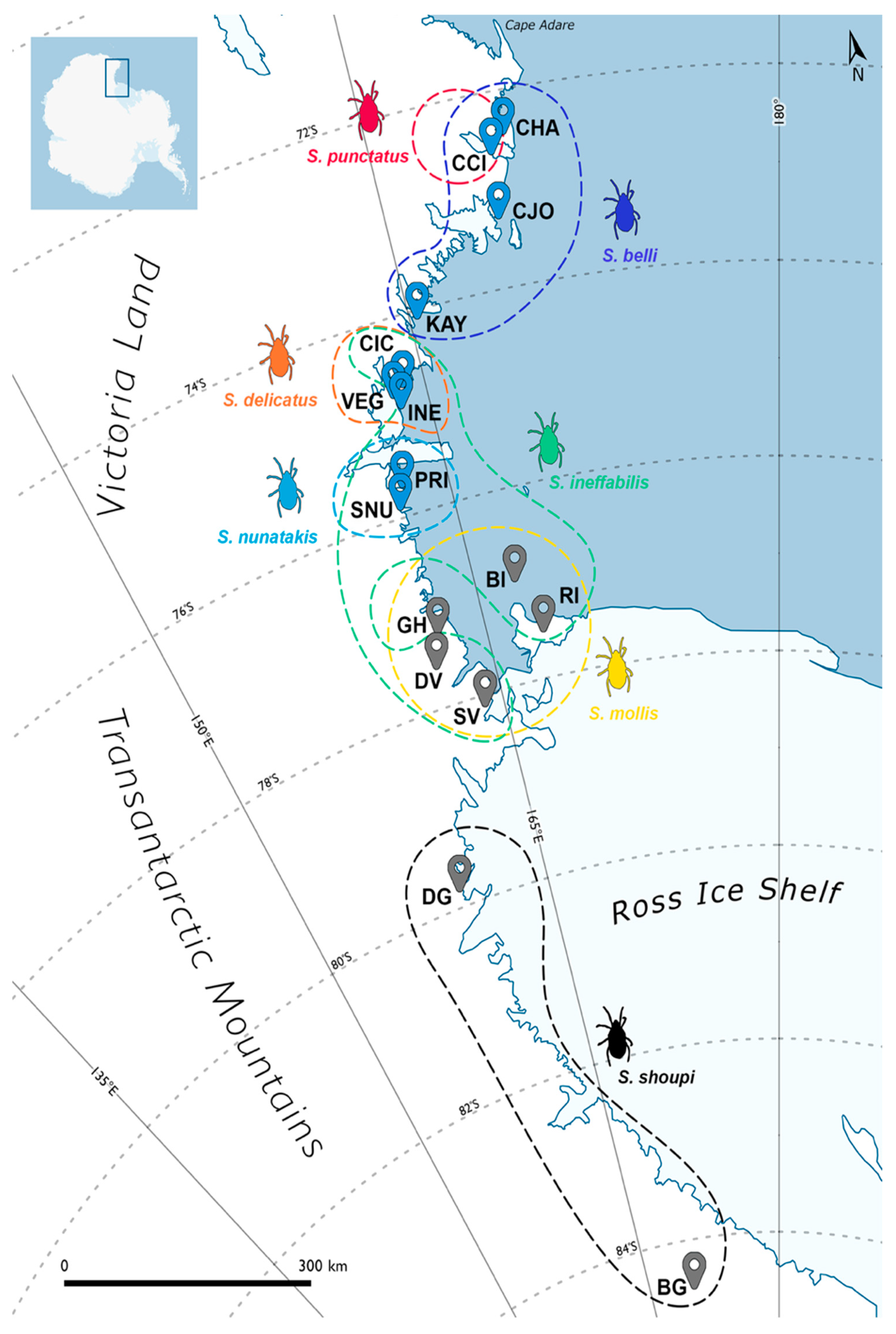
2.1. Sample Collection
2.2. Molecular Dataset
2.3. Combined Morphological Analysis
2.4. Phylogenetic Analyses
2.5. Population Structure Analyses
3. Results
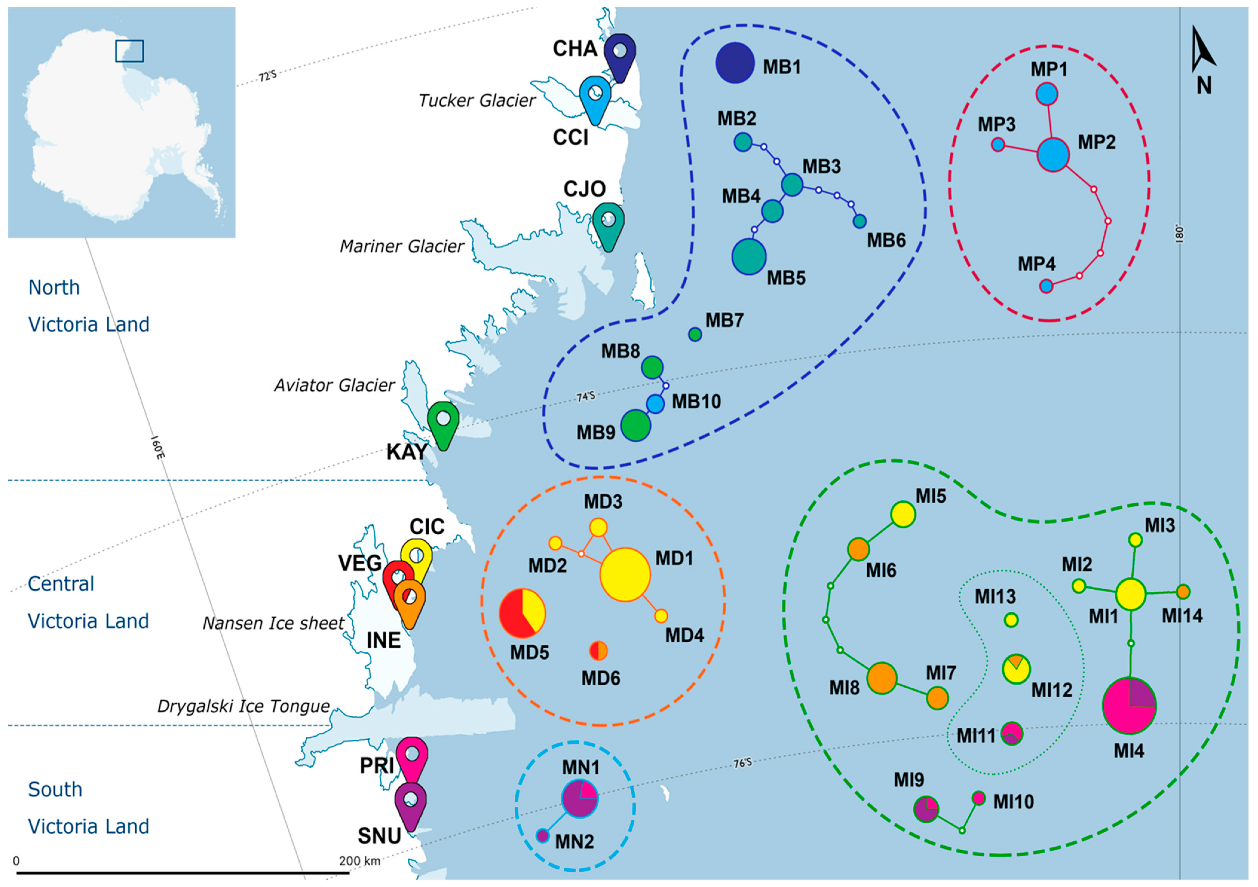
3.1. Haplotype Network Analyses
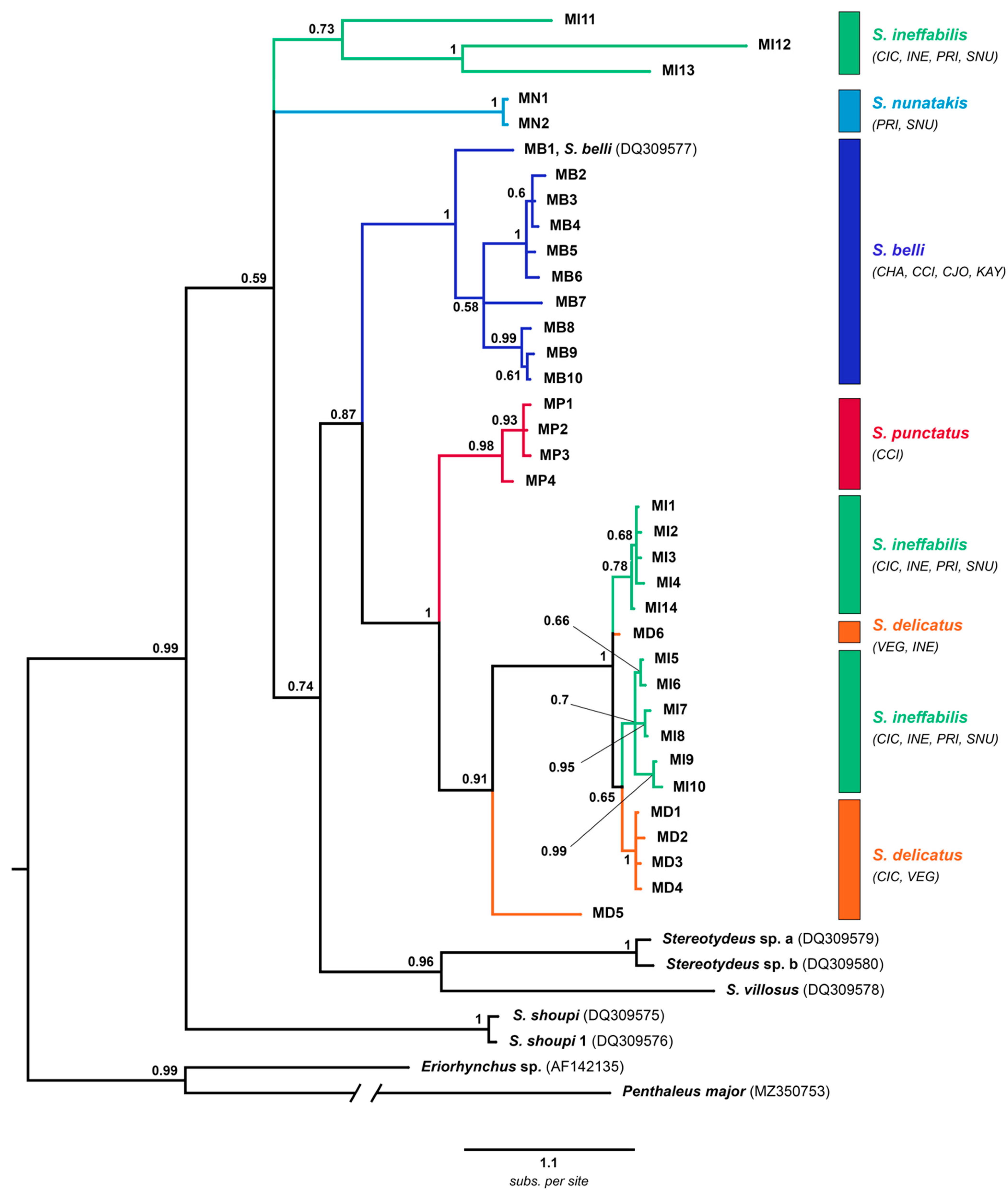
3.2. Phylogenetic Analyses
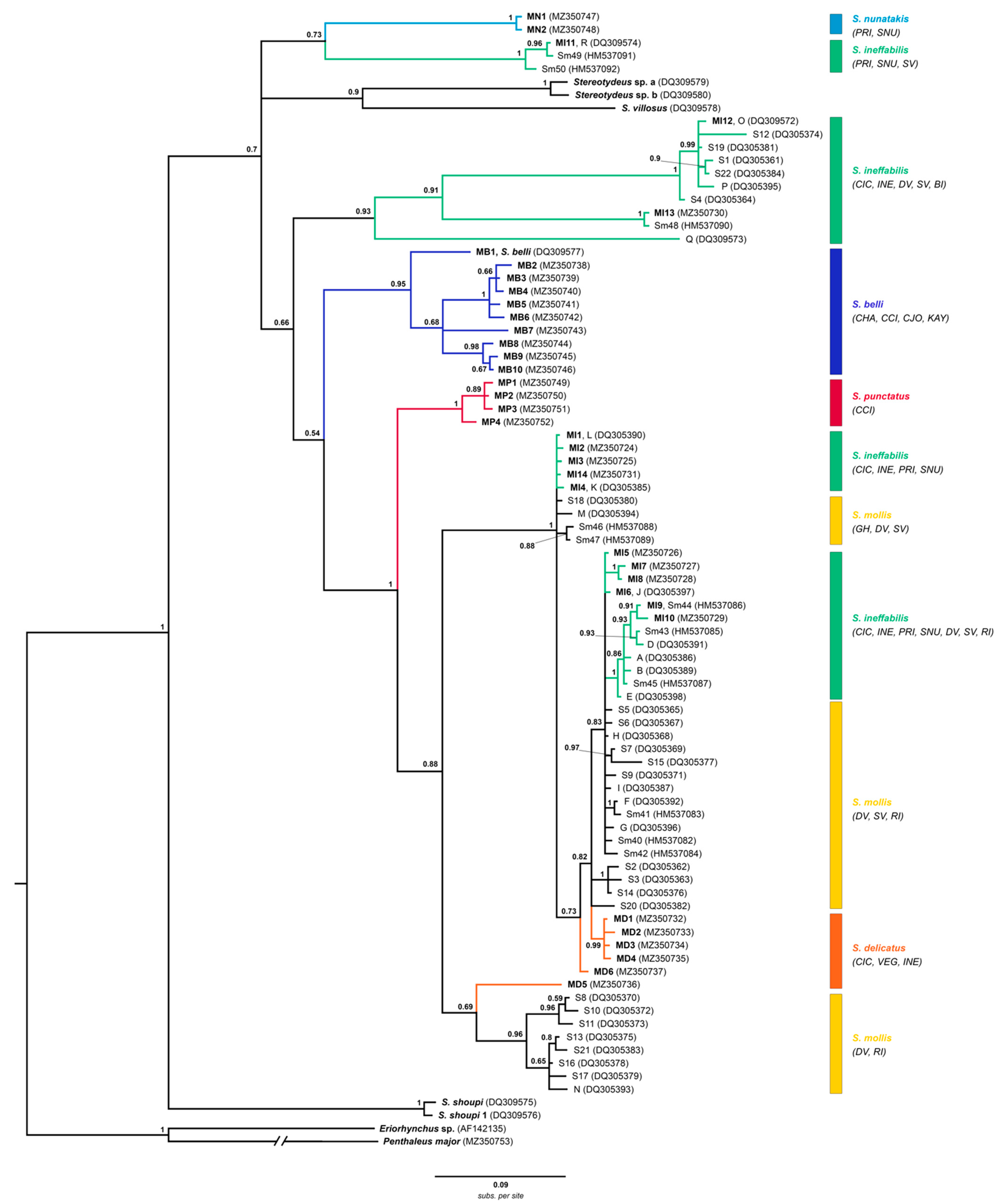
- cox1 with outgroups
- cox1 all haplotypes
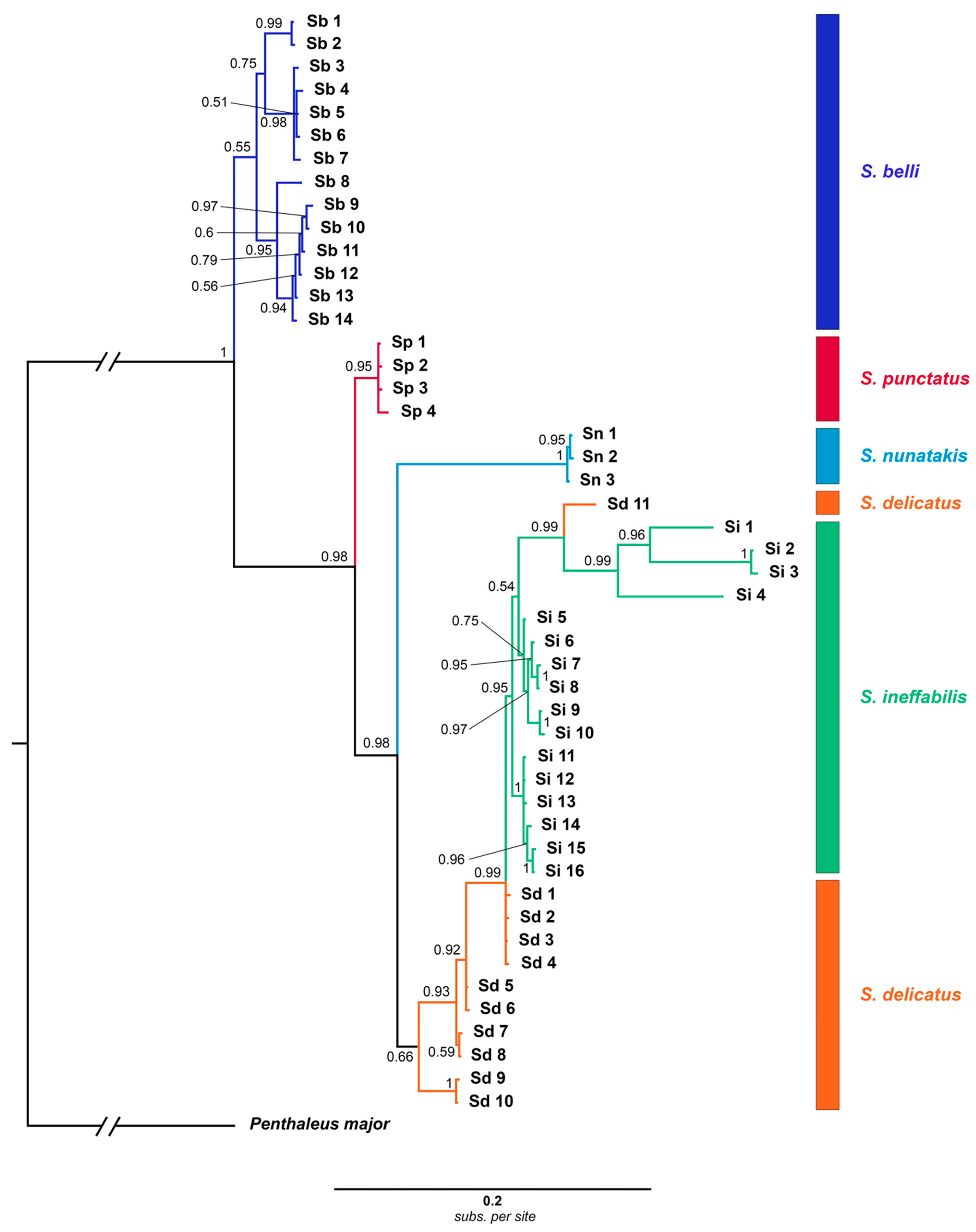
- Combined cox1-28S
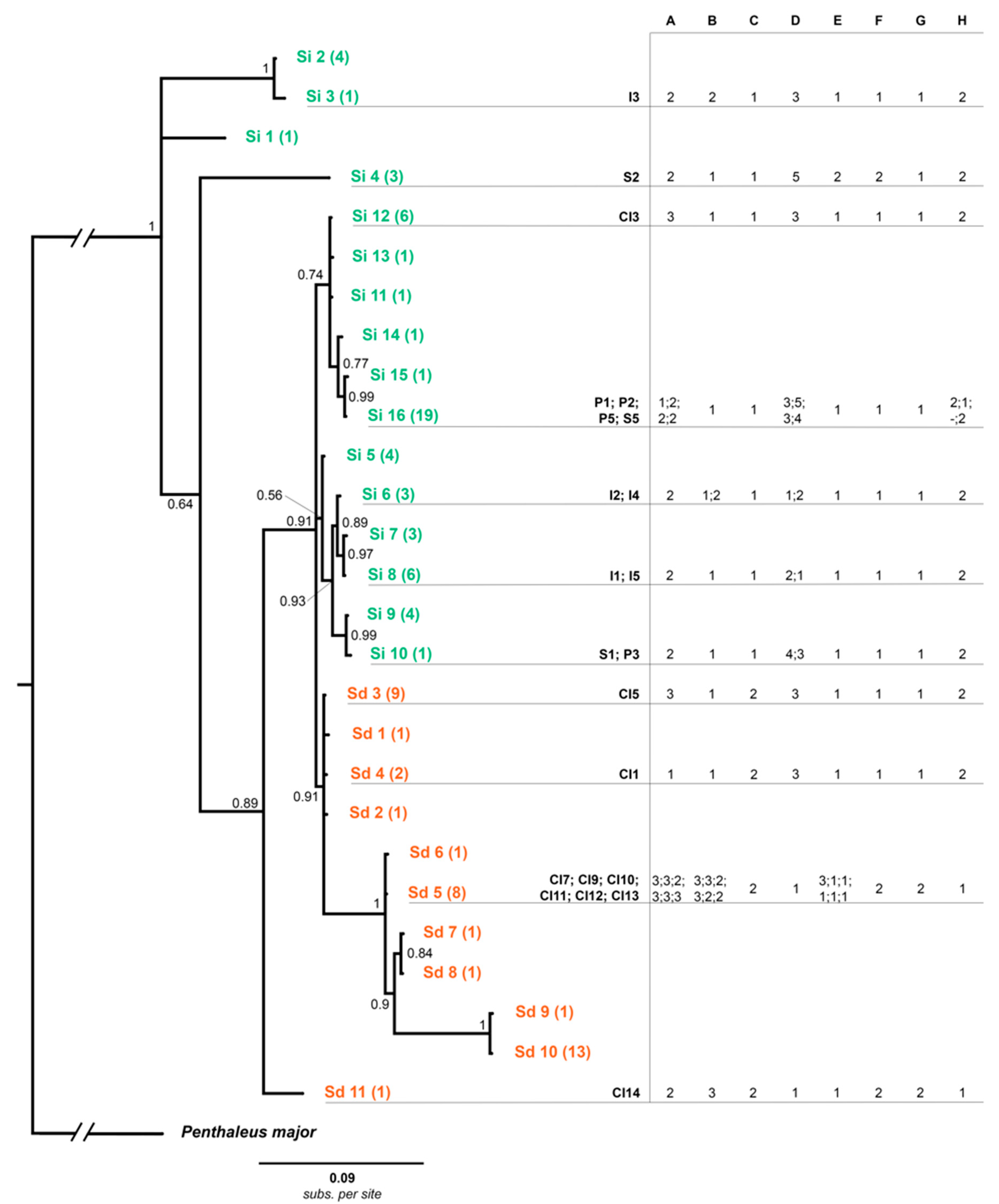
- Combined cox1-28S with morphology
3.3. Population Structure Analyses
4. Discussion
4.1. North Victoria Land Taxa
4.2. Central-South Victoria Land Taxa
4.3. Speciation in Action
Supplementary Materials
Author Contributions
Funding
Institutional Review Board Statement
Data Availability Statement
Acknowledgments
Conflicts of Interest
References
- Block, W. Terrestrial Microbiology, Invertebrates and Ecosystems. In Antarctic Ecology; R. M. Laws: London, UK, 1984. [Google Scholar]
- Convey, P. Antarctic Ecosystems. In Encyclopedia of Biodiversity; Levin, S., Ed.; Academic Press: San Diego, CA, USA, 2017; Volume 1, pp. 179–187. [Google Scholar]
- Spain, A.V. Some Aspects of Soil Conditions and Arthropod Distribution in Antarctica. Pac. Insects Monogr. 1971, 25, 21–26. [Google Scholar]
- Schwarz, A.-M.J.; Green, J.D.; Green, T.G.A.; Seppelt, R.D. Invertebrates Associated with Moss Communities at Canada Glacier, Southern Victoria Land, Antarctica. Polar Biol. 1993, 13, 157–162. [Google Scholar] [CrossRef]
- Kennedy, A.D. Water as a Limiting Factor in the Antarctic Terrestrial Environment: A Biogeographical Synthesis. Arct. Alp. Res. 1993, 25, 308–315. [Google Scholar] [CrossRef]
- Skotnicki, M.L.; Selkirk, P.M. Plant Biodiversity in an Extreme Environment. In Trends in Antarctic Terrestrial and Limnetic Ecosystems: Antarctica as a Global Indicator; Bergstrom, D.M., Convey, P., Huiskes, A.H.L., Eds.; Springer: Dordrecht, The Netherlands, 2006; pp. 161–175. ISBN 978-1-4020-5277-4. [Google Scholar]
- Marshall, D.J.; Pugh, P.J.A. Origin of the Inland Acari of Continental Antarctica, with Particular Reference to Dronning Maud. Zool. J. Linn. 1996, 118, 101–118. [Google Scholar] [CrossRef]
- Convey, P.; Peck, L.S. Antarctic Environmental Change and Biological Responses. Sci. Adv. 2019, 5, eaaz0888. [Google Scholar] [CrossRef]
- Cannon, R.J.C.; Block, W. Cold Tolerance of Microarthropods. Biol. Rev. 1988, 63, 23–77. [Google Scholar] [CrossRef]
- Block, W.; Baust, J.G.; Franks, F.; Johnston, I.A.; Bale, J. Cold Tolerance of Insects and Other Arthropods. Philos. Trans. R. Soc. Lond. B Biol. Sci. 1990, 326, 613–633. [Google Scholar]
- Sinclair, B.J.; Sjursen, H. Terrestrial Invertebrate Abundance across a Habitat Transect in Keble Valley, Ross Island, Antarctica. Pedobiologia 2001, 45, 134–145. [Google Scholar] [CrossRef]
- Sjursen, H.; Sinclair, B.J. On the Cold Hardiness of Stereotydeus mollis (Acari: Prostigmata) from Ross Island, Antarctica. Pedobiologia 2002, 46, 188–195. [Google Scholar] [CrossRef]
- Caruso, T.; Bargagli, R. Assessing Abundance and Diversity Patterns of Soil Microarthropod Assemblages in Northern Victoria Land (Antarctica). Polar Biol. 2007, 30, 895–902. [Google Scholar] [CrossRef]
- Janetschek, H. Arthropod Ecology of South Victoria Land. Antarct. Res. Ser. 1967, 10, 205–293. [Google Scholar]
- Gressitt, J.L. Introduction: Dispersal. In Entomology of Antarctica; Gressitt, J.L., Ed.; Antarctic Research Series; American Geophysical Union: Washington, DC, USA, 1967; Volume 10, pp. 25–27. [Google Scholar]
- Coulson, S.J.; Hodkinson, I.D.; Webb, N.R.; Harrison, J.A. Survival of Terrestrial Soil-Dwelling Arthropods on and in Seawater: Implications for Trans-Oceanic Dispersal. Funct. Ecol. 2002, 16, 353–356. [Google Scholar] [CrossRef]
- Hawes, T.C.; Worland, M.R.; Bale, J.S.; Convey, P. Rafting in Antarctic Collembola. J. Zool. 2008, 274, 44–50. [Google Scholar] [CrossRef]
- Hawes, T.C. Rafting in the Antarctic Springtail, Gomphiocephalus hodgsoni. Antarct. Sci. 2011, 23, 456–460. [Google Scholar] [CrossRef]
- Pugh, P.J.A. Acarine Colonisation of Antarctica and the Islands of the Southern Ocean: The Role of Zoohoria. Polar Rec. 1997, 33, 113–122. [Google Scholar] [CrossRef]
- Strong, J. Ecology of Terrestrial Arthropods at Palmer Station, Antarctic Peninsula. In Entomology of Antarctica; Gressitt, J.L., Ed.; Antarctic Research Series; American Geophysical Union: Washington, DC, USA, 1967; Volume 10, pp. 357–371. ISBN 978-1-118-66869-6. [Google Scholar]
- Tilbrook, P.J. Arthropod Ecology in the Maritime Antarctic. In Entomology of Antarctica; Gressitt, J.L., Ed.; Antarctic Research Series; American Geophysical Union: Washington, DC, USA, 1967; Volume 10, pp. 331–356. ISBN 978-1-118-66869-6. [Google Scholar]
- Stevens, M.I.; Hogg, I.D. Long-Term Isolation and Recent Range Expansion from Glacial Refugia Revealed for the Endemic Springtail Gomphiocephalus hodgsoni from Victoria Land, Antarctica. Mol. Ecol. 2003, 12, 2357–2369. [Google Scholar] [CrossRef]
- Wallwork, J.A. Distribution Patterns of Cryptostigmatid Mites (Arachnida: Acari) in South Georgia. Pac. Insects 1972, 14, 615–625. [Google Scholar]
- Lehmitz, R.; Russell, D.; Hohberg, K.; Christian, A.; Xylander, W.E.R. Wind Dispersal of Oribatid Mites as a Mode of Migration. Pedobiologia 2011, 54, 201–207. [Google Scholar] [CrossRef]
- Pugh, P.J.A. Have Mites (Acarina: Arachnida) Colonised Antarctica and the Islands of the Southern Ocean via Air Currents? Polar Rec. 2003, 39, 239–244. [Google Scholar] [CrossRef]
- Hawes, T.C.; Worland, M.R.; Convey, P.; Bale, J.S. Aerial Dispersal of Springtails on the Antarctic Peninsula: Implications for Local Distribution and Demography. Antarct. Sci. 2007, 19, 3–10. [Google Scholar] [CrossRef]
- Fanciulli, P.P.; Summa, D.; Dallai, R.; Frati, F. High Levels of Genetic Variability and Population Differentiation in Gressittacantha terranova (Collembola, Hexapoda) from Victoria Land, Antarctica. Antarct. Sci. 2001, 13, 246–254. [Google Scholar] [CrossRef]
- Frati, F.; Spinsanti, G.; Dallai, R. Genetic Variation of MtCOII Gene Sequences in the Collembolan Isotoma klovstadi from Victoria Land, Antarctica: Evidence for Population Differentiation. Polar Biol. 2001, 24, 934–940. [Google Scholar] [CrossRef]
- Torricelli, G.; Carapelli, A.; Convey, P.; Nardi, F.; Boore, J.L.; Frati, F. High Divergence across the Whole Mitochondrial Genome in the “Pan-Antarctic” Springtail Friesea grisea: Evidence for Cryptic Species? Gene 2010, 449, 30–40. [Google Scholar] [CrossRef]
- Torricelli, G.; Frati, F.; Convey, P.; Telford, M.; Carapelli, A. Population Structure of Friesea grisea (Collembola, Neanuridae) in the Antarctic Peninsula and Victoria Land: Evidence for Local Genetic Differentiation of Pre-Pleistocene Origin. Antarct. Sci. 2010, 22, 757–765. [Google Scholar] [CrossRef]
- Carapelli, A.; Greenslade, P.; Nardi, F.; Leo, C.; Convey, P.; Frati, F.; Fanciulli, P.P. Evidence for Cryptic Diversity in the “Pan-Antarctic” Springtail Friesea antarctica and the Description of Two New Species. Insects 2020, 11, 141. [Google Scholar] [CrossRef] [PubMed]
- Stevens, M.I.; Greenslade, P.; Hogg, I.D.; Sunnucks, P. Southern Hemisphere Springtails: Could Any Have Survived Glaciation of Antarctica? Mol. Biol. Evol. 2006, 23, 874–882. [Google Scholar] [CrossRef] [PubMed]
- Stevens, M.I.; Hogg, I.D. Contrasting Levels of Mitochondrial DNA Variability between Mites (Penthalodidae) and Springtails (Hypogastruridae) from the Trans-Antarctic Mountains Suggest Long-Term Effects of Glaciation and Life History on Substitution Rates, and Speciation Processes. Soil Biol. Biochem. 2006, 38, 3171–3180. [Google Scholar] [CrossRef]
- McGaughran, A.; Hogg, I.D.; Stevens, M.I. Patterns of Population Genetic Structure for Springtails and Mites in Southern Victoria Land, Antarctica. Mol. Phylogenet. Evol. 2008, 46, 606–618. [Google Scholar] [CrossRef]
- McGaughran, A.; Torricelli, G.; Carapelli, A.; Frati, F.; Stevens, M.I.; Convey, P.; Hogg, I.D. Contrasting Phylogeographical Patterns for Springtails Reflect Different Evolutionary Histories between the Antarctic Peninsula and Continental Antarctica. J. Biogeogr. 2010, 37, 103–119. [Google Scholar] [CrossRef]
- Demetras, N.J.; Hogg, I.D.; Banks, J.C.; Adams, B.J. Latitudinal Distribution and Mitochondrial DNA (COI) Variability of Stereotydeus spp. (Acari: Prostigmata) in Victoria Land and the Central Transantarctic Mountains. Antarct. Sci. 2010, 22, 749–756. [Google Scholar] [CrossRef]
- Martin, A.P.; Palumbi, S.R. Body Size, Metabolic Rate, Generation Time, and the Molecular Clock. Proc. Natl. Acad. Sci. USA 1993, 90, 4087–4091. [Google Scholar] [CrossRef]
- Sinclair, B.J.; Stevens, M.I. Terrestrial Microarthropods of Victoria Land and Queen Maud Mountains, Antarctica: Implications of Climate Change. Soil Biol. Biochem. 2006, 38, 3158–3170. [Google Scholar] [CrossRef]
- Convey, P.; Biersma, E.M.; Casanova-Katny, A.; Maturana, C.S. Chapter 10—Refuges of Antarctic diversity. In Past Antarctica; Oliva, M., Ruiz-Fernández, J., Eds.; Academic Press: London, UK, 2020; pp. 181–200. ISBN 978-0-12-817925-3. [Google Scholar]
- Gressitt, J.L.; Shoup, J. Ecological Notes on Free-Living Mites in North Victoria Land. In Entomology of Antarctica; Gressitt, J.L., Ed.; Antarctic Research Series; American Geophysical Union: Washington, DC, USA, 1967; Volume 10, pp. 307–320. [Google Scholar]
- Greenslade, P. An Antarctic Biogeographical Anomaly Resolved: The True Identity of a Widespread Species of Collembola. Polar Biol. 2018, 41, 969–981. [Google Scholar] [CrossRef]
- Greenslade, P. A New Species of Friesea (Collembola: Neanuridae) from the Antarctic Continent. J. Nat. Hist. 2018, 52, 2197–2207. [Google Scholar] [CrossRef]
- Womersley, H.; Strandtmann, R.W. On Some Free Living Prostigmatic Mites of Antarctica. Pac. Insects 1963, 5, 451–472. [Google Scholar]
- Strandtmann, R.W. Terrestrial Prostigmata (trombidiform mites). In Antarctic Research Series; Gressitt, J.L., Ed.; American Geophysical Union: Washington, DC, USA, 1967; pp. 51–80. ISBN 978-1-118-66869-6. [Google Scholar]
- Pittard, D.A. A Comparative Study of the Life Stages of the Mite, Stereotydeus mollis W. & S. (Acarina). Pac. Insects Monogr. 1971, 25, 1–14. [Google Scholar]
- Fitzsimons, J.M. Temperature and Three Species of Antarctic Arthropods. Pac. Insects Monogr. 1971, 25, 127–135. [Google Scholar]
- Block, W. Ecological and Physiological Studies of Terrestrial Arthropods in the Ross Dependency 1984-85. Brit. Antarct. Surv. Bull. 1985, 68, 115–122. [Google Scholar]
- Brunetti, C.; Siepel, H.; Fanciulli, P.P.; Nardi, F.; Convey, P.; Carapelli, A. Two New Species of the Mite Genus Stereotydeus Berlese, 1901 (Prostigmata: Penthalodidae) from Victoria Land, and a Key for Identification of Antarctic and Sub-Antarctic Species. Taxonomy 2021, 1, 116–141. [Google Scholar] [CrossRef]
- Xiao, J.-H.; Wang, N.-X.; Li, Y.-W.; Murphy, R.W.; Wan, D.-G.; Niu, L.-M.; Hu, H.-Y.; Fu, Y.-G.; Huang, D.-W. Molecular Approaches to Identify Cryptic Species and Polymorphic Species within a Complex Community of Fig Wasps. PLoS ONE 2010, 5, e15067. [Google Scholar] [CrossRef]
- Jörger, K.M.; Schrödl, M. How to Describe a Cryptic Species? Practical Challenges of Molecular Taxonomy. Front. Zool. 2013, 10, 59. [Google Scholar] [CrossRef] [PubMed]
- Chown, S.L.; Lee, J.E.; Hughes, K.A.; Barnes, J.; Barrett, P.J.; Bergstrom, D.M.; Convey, P.; Cowan, D.A.; Crosbie, K.; Dyer, G.; et al. Challenges to the Future Conservation of the Antarctic. Science 2012, 337, 158–159. [Google Scholar] [CrossRef] [PubMed]
- Lee, J.R.; Raymond, B.; Bracegirdle, T.J.; Chadès, I.; Fuller, R.A.; Shaw, J.D.; Terauds, A. Climate Change Drives Expansion of Antarctic Ice-Free Habitat. Nature 2017, 547, 49–54. [Google Scholar] [CrossRef] [PubMed]
- Bergami, E.; Rota, E.; Caruso, T.; Birarda, G.; Vaccari, L.; Corsi, I. Plastics Everywhere: First Evidence of Polystyrene Fragments inside the Common Antarctic Collembolan Cryptopygus antarcticus. Biol. Lett. 2020, 16, 20200093. [Google Scholar] [CrossRef] [PubMed]
- Carapelli, A.; Convey, P.; Frati, F.; Spinsanti, G.; Fanciulli, P.P. Population Genetics of Three Sympatric Springtail Species (Hexapoda: Collembola) from the South Shetland Islands: Evidence for a Common Biogeographic Pattern. Biol. J. Linn. Soc. 2017, 120, 788–803. [Google Scholar] [CrossRef]
- Wauchope, H.S.; Shaw, J.D.; Terauds, A. A Snapshot of Biodiversity Protection in Antarctica. Nat. Commun. 2019, 10, 946. [Google Scholar] [CrossRef]
- Terauds, A.; Chown, S.L.; Morgan, F.; Peat, H.J.; Watts, D.J.; Keys, H.; Convey, P.; Bergstrom, D.M. Conservation Biogeography of the Antarctic. Divers. Distrib. 2012, 18, 726–741. [Google Scholar] [CrossRef]
- Terauds, A.; Lee, J.R. Antarctic Biogeography Revisited: Updating the Antarctic Conservation Biogeographic Regions. Divers. Distrib. 2016, 22, 836–840. [Google Scholar] [CrossRef]
- Hawes, T.C.; Torricelli, G.; Stevens, M.I. Haplotype Diversity in the Antarctic Springtail Gressittacantha terranova at Fine Spatial Scales - A Holocene Twist to a Pliocene Tale. Antarct. Sci. 2010, 22, 766–773. [Google Scholar] [CrossRef]
- Carapelli, A.; Leo, C.; Frati, F. High Levels of Genetic Structuring in the Antarctic Springtail Cryptopygus terranovus. Antarct. Sci. 2017, 29, 311–323. [Google Scholar] [CrossRef]
- Matsuoka, K.; Skoglund, A.; Roth, G. Quantarctica [Dataset]. Nor. Polar Inst. 2018, 10. Available online: https://www.npolar.no/quantarctica/ (accessed on 25 June 2021).
- Otto, J.C.; Wilson, K.J. Assessment of the Usefulness of Ribosomal 18S and Mitochondrial COI Sequences in Prostigmata Phylogeny. In Acarology: Proceedings of the 10th International Congress; CSIRO Publishing: Melbourne, Australia, 2001; Volume 100. [Google Scholar]
- Friedrich, M.; Tautz, D. An Episodic Change of RDNA Nucleotide Substitution Rate Has Occurred during the Emergence of the Insect Order Diptera. Mol. Biol. Evol. 1997, 14, 644–653. [Google Scholar] [CrossRef] [PubMed]
- MacVector, Inc. MacVector; MacVector, Inc.: Apex, NC, USA, 2018. [Google Scholar]
- Collins, G.E.; Hogg, I.D.; Convey, P.; Barnes, A.D.; McDonald, I.R. Spatial and Temporal Scales Matter When Assessing the Species and Genetic Diversity of Springtails (Collembola) in Antarctica. Front. Ecol. Evol. 2019, 7, 76. [Google Scholar] [CrossRef]
- Sievers, F.; Wilm, A.; Dineen, D.; Gibson, T.J.; Karplus, K.; Li, W.; Lopez, R.; McWilliam, H.; Remmert, M.; Söding, J.; et al. Fast, Scalable Generation of High-quality Protein Multiple Sequence Alignments Using Clustal Omega. Mol. Syst. Biol. 2011, 7, 539. [Google Scholar] [CrossRef] [PubMed]
- Villesen, P. FaBox: An Online Toolbox for Fasta Sequences. Mol. Ecol. Notes 2007, 7, 965–968. [Google Scholar] [CrossRef]
- Castresana, J. Selection of Conserved Blocks from Multiple Alignments for Their Use in Phylogenetic Analysis. Mol. Biol. Evol. 2000, 17, 540–552. [Google Scholar] [CrossRef]
- R Core Team R: The R Project for Statistical Computing. 2016. Available online: https://oasishub.co/dataset/the-r-project-for-statistical-computing (accessed on 16 March 2021).
- Paradis, E.; Schliep, K. Ape 5.0: An Environment for Modern Phylogenetics and Evolutionary Analyses in R. Bioinformatics 2019, 35, 526–528. [Google Scholar] [CrossRef] [PubMed]
- Lanfear, R.; Frandsen, P.B.; Wright, A.M.; Senfeld, T.; Calcott, B. PartitionFinder 2: New Methods for Selecting Partitioned Models of Evolution for Molecular and Morphological Phylogenetic Analyses. Mol. Biol. Evol. 2016, 34, 772–773. [Google Scholar] [CrossRef]
- Ronquist, F.; Teslenko, M.; van der Mark, P.; Ayres, D.L.; Darling, A.; Höhna, S.; Larget, B.; Liu, L.; Suchard, M.A.; Huelsenbeck, J.P. MrBayes 3.2: Efficient Bayesian Phylogenetic Inference and Model Choice Across a Large Model Space. Syst. Biol. 2012, 61, 539–542. [Google Scholar] [CrossRef]
- Rambaut, A. FigTree v 1.4. 2012. Available online: http://tree.bio.ed.ac.uk/software/figtree/ (accessed on 21 April 2021).
- Clement, M.; Posada, D.; Crandall, K. TCS: A Computer Program to Estimate Gene Genealogies. Mol. Ecol. 2000, 9, 1657–1659. [Google Scholar] [CrossRef]
- Múrias dos Santos, A.; Cabezas, M.P.; Tavares, A.I.; Xavier, R.; Branco, M. TcsBU: A Tool to Extend TCS Network Layout and Visualization. Bioinformatics 2016, 32, 627–628. [Google Scholar] [CrossRef] [PubMed]
- Excoffier, L.; Laval, G.; Schneider, S. Arlequin (Version 3.0): An Integrated Software Package for Population Genetics Data Analysis. Evol. Bioinform. 2005, 1, 47–50. [Google Scholar] [CrossRef]
- Nei, M. Molecular Evolutionary Genetics; Columbia University Press: New York, NY, USA, 1987. [Google Scholar]
- Excoffier, L.; Smouse, P.E.; Quattro, J.M. Analysis of Molecular Variance Inferred from Metric Distances among DNA Haplotypes: Application to Human Mitochondrial DNA Restriction Data. Genetics 1992, 131, 479–491. [Google Scholar] [CrossRef] [PubMed]
- Wise, K.A.J. Collembola (springtails). In Entomology of Antarctica; Gressitt, J.L., Ed.; Antarctic Research Series; American Geophysical Union: Washington, DC, USA, 1967; pp. 123–148. [Google Scholar]
- Knowles, L.L. Did the Pleistocene Glaciations Promote Divergence? Tests of Explicit Refugial Models in Montane Grasshoppers. Mol. Ecol. 2001, 10, 691–701. [Google Scholar] [CrossRef] [PubMed]
- Rowe, K.C.; Heske, E.J.; Brown, P.W.; Paige, K.N. Surviving the Ice: Northern Refugia and Postglacial Colonization. Proc. Natl. Acad. Sci. USA 2004, 101, 10355–10359. [Google Scholar] [CrossRef] [PubMed]
- Huiskes, A.H.L.; Convey, P.; Bergstrom, D.M. Trends in Antarctic Terrestrial and Limnetic Ecosystems: Antarctica as a Global Indicator. In Trends in Antarctic Terrestrial and Limnetic Ecosystems: Antarctica as a Global Indicator; Bergstrom, D.M., Convey, P., Huiskes, A.H.L., Eds.; Springer: Dordrecht, The Netherlands, 2006; pp. 1–13. ISBN 978-1-4020-5277-4. [Google Scholar]
- Via, S. Sympatric Speciation in Animals: The Ugly Duckling Grows Up. Trends Ecol. Evol. 2001, 16, 381–390. [Google Scholar] [CrossRef]
- Nosil, P. Ecological Speciation; Oxford University Press: Oxford, UK, 2012. [Google Scholar]
- Foote, A.D. Sympatric Speciation in the Genomic Era. Trends Ecol. Evol. 2018, 33, 85–95. [Google Scholar] [CrossRef]
- Rundle, H.D.; Nosil, P. Ecological Speciation. Ecol. Lett. 2005, 8, 336–352. [Google Scholar] [CrossRef]
- Schluter, D. Evidence for Ecological Speciation and Its Alternative. Science 2009, 323, 737–741. [Google Scholar] [CrossRef]
- McGaughran, A.; Redding, G.P.; Stevens, M.I.; Convey, P. Temporal Metabolic Rate Variation in a Continental Antarctic Springtail. J. Insect Physiol. 2009, 55, 130–135. [Google Scholar] [CrossRef]

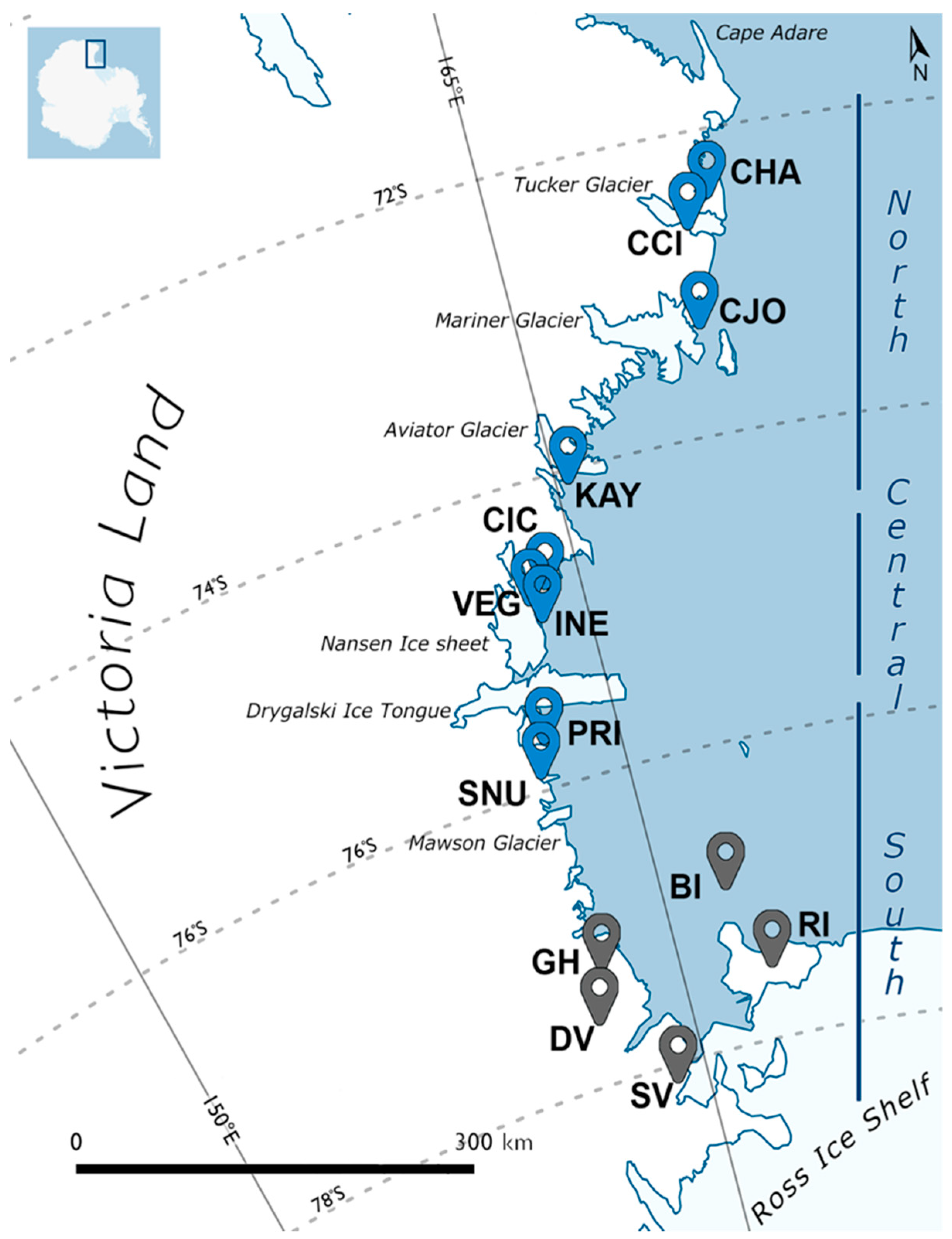
| ID | Locality | Victoria Land | Lat (S) | Long (E) | Altitude | n. | Species |
|---|---|---|---|---|---|---|---|
| CHA | Cape Hallett (Adelie Cove) | North | 72°26′25″ | 169°56′32″ | 140 m | 10 | S. belli |
| CCI | Crater Cirque | North | 72°37′52″ | 169°22′22″ | 200 m | 14 | S. belli; S. punctatus |
| CJO | Cape Jones | North | 73°16′38″ | 169°12′54″ | 310 m | 17 | S. belli |
| KAY | Kay Island | North | 74°04′14″ | 165°18′60″ | 140 m | 10 | S. belli |
| CIC | Campo Icaro | Central * | 74°42′45″ | 164°06′21″ | 70 m | 35 | S. ineffabilis; S. delicatus |
| VEG | Vegetation Island | Central * | 74°47′00″ | 163°37′00″ | 120 m | 10 | S. delicatus |
| INE | Inexpressible Island | Central * | 74°53′39″ | 163°43′44″ | 30 m | 10 | S. ineffabilis; S. delicatus |
| PRI | Prior Island | South | 75°41′31″ | 162°52′34″ | 130 m | 17 | S. ineffabilis; S. nunatakis |
| SNU | Starr Nunatak | South | 75°53′57″ | 162°35′08″ | 60 m | 14 | S. ineffabilis; S. nunatakis |
| Locality | ID | Date | Slide | Sex | Species |
|---|---|---|---|---|---|
| Campo Icaro | CIC | 28 January 2019 | CI1 | M | S. delicatus |
| CI3 | F | S. ineffabilis | |||
| CI5 | F | S. delicatus | |||
| CI7 | M | S. delicatus | |||
| 24 December 2017 | CI9 | M | S. delicatus | ||
| CI10 | M | ||||
| CI11 | F | ||||
| CI12 | F | ||||
| CI13 | F | ||||
| CI14 | M | ||||
| Inexpressible Island | INE | 21 January 2019 | I1 | F | S. ineffabilis |
| I2 | M | ||||
| I3 | F | ||||
| I4 | M | ||||
| I5 | F | ||||
| Prior Island | PRI | 11 January 2019 | P1 | M | S. ineffabilis |
| P2 | M | ||||
| P3 | F | ||||
| P5 | M | ||||
| Starr Nunatak | SNU | 11 January 2018 | S1 | M | S. ineffabilis |
| S2 | M | ||||
| S5 | F |
| n. | Single/Multi Locus | cox1 | 28S | Ref. | Outgroups | Best Model | |||||
|---|---|---|---|---|---|---|---|---|---|---|---|
| 1st | 2nd | 3rd | Non-Cod | ||||||||
| i | cox1 with outgroups | 159 | single | x | - | S. shoupi (2) | Eriorhynchus sp. P. major | K81UF+I+G | GTR+I | F81+I | - |
| S. villosus | |||||||||||
| Stereotydeus sp. (2) | |||||||||||
| S. belli | |||||||||||
| ii | cox1 all haplotypes | 159 | single | x | - | S. shoupi (2) | Eriorhynchus sp. P. major | K81UF+G | GTR+I+G | F81+I | - |
| S. villosus | |||||||||||
| Stereotydeus sp. (2) | |||||||||||
| S. belli | |||||||||||
| S. mollis (50) | |||||||||||
| iii | combined cox1-28S | 159 | multi | x | x | - | P. major | K81UF+I+G | TRN+I | F81+I | GTR+G |
| iv | combined cox1-28S with morphologica information | 99 | multi | x | x | - | P. major | HKY+I+G | TIM+G | F81+G | TVM+G |
| Species | Specimens | Haplotypes | ||
|---|---|---|---|---|
| cox1 | 28S | Combined | ||
| S. belli | 39 | 10 | 9 | 14 |
| S. punctatus | 12 | 4 | 1 | 4 |
| S. ineffabilis | 59 | 14 | 3 | 16 |
| S. delicatus | 39 | 6 | 2 | 10 |
| S. nunatakis | 10 | 2 | 2 | 3 |
| ID | n. | N. | Species | Haplotypes | ||
|---|---|---|---|---|---|---|
| cox1 | 28S | Combined | ||||
| CHA | 10 | 1 | S. belli | MB1(10) | RB1(9), RB2(1) | Sb1(9), Sb2(1) |
| CCI | 14 | 2 | S. belli | MB10(2) | RB8(1), RB9(1) | Sb12(1), Sb13(1) |
| S. punctatus | MP1(3), MP2(7), MP3(1), MP4(1) | RP1(12) | Sp1(7), Sp2(3), Sp3(1), Sp4(1) | |||
| CJO | 17 | 1 | S. belli | MB2(2), MB3(3), MB4(3), MB5(8), MB6(1) | RB3(16), RB4(1) | Sb3(8), Sb4(2), Sb5(3), Sb6(3), Sb7(1) |
| KAY | 10 | 1 | S. belli | MB7(1), MB8(3), MB9(6) | RB5(7), RB6(1), RB7(1), RB8(1) | Sb8(1), Sb9(2), Sb10(5), Sb11(1), Sb14(1) |
| CIC | 45 | 2 | S. delicatus | MD1(18), MD2(1), MD3(2), MD4(1), MD5(6) | RD1(12), RD2(2), RX1(14) | Sd1(1), Sd2(1), Sd3(9), Sd4(2), Sd5(8), Sd6(1), Sd9(1), Sd10(4), Sd11(1) |
| S. ineffabilis | MI1(6), MI2(1), MI3(1), MI5(4), MI12(4), MI13(1) | RX1(17) | Si1(1), Si2(4), Si5(4), Si11(1), Si12(6), Si13(1) | |||
| VEG | 10 | 1 | S. delicatus | MD5(9), MD6(1) | RD1(10) | Sd8(1), Sd10(9) |
| INE | 15 | 2 | S. delicatus | MD6(1) | RD2(1) | Sd7(1) |
| S. ineffabilis | MI6(3), MI7(3), MI8(6), MI12(1), MI14(1) | RI1(14) | Si3(1), Si6(3), Si7(3), Si8(6), Si14(1) | |||
| PRI | 21 | 2 | S. ineffabilis | MI4(15), MI9(1), MI10(1), MI11(2) | RI3(19) | Si4(2), Si9(1), Si10(1), Si16(15) |
| S. nunatakis | MN1(2) | RN1(2) | Sn1(2) | |||
| SNU | 17 | 2 | S. ineffabilis | MI4(5), MI9(3), MI11(1) | RI2(1), RI3(8) | Si4(1), Si9(3), Si15(1), Si16(4) |
| S. nunatakis | MN1(7), MN2(1) | RN1(7), RN2(1) | Sn1(6), Sn2(1), Sn3(1) | |||
| MI4 | MI1 | MI2 | MI3 | MI14 | MI5 | MI9 | MI10 | MI6 | MI8 | MI7 | MD6 | MD1 | MD4 | MD3 | MD2 | MD5 | MP3 | MP4 | MP2 | MP1 | MB10 | MB9 | MB8 | MB7 | MB1, S. belli | MB6 | MB5 | MB3 | MB4 | MB2 | MN1 | MN2 | MI12 | MI13 | MI11 | Stereotydeus sp.a | Stereotydeus sp.b | S. villosus | S. shoupi | S. shoupi 1 | |
|---|---|---|---|---|---|---|---|---|---|---|---|---|---|---|---|---|---|---|---|---|---|---|---|---|---|---|---|---|---|---|---|---|---|---|---|---|---|---|---|---|---|
| MI4 | 0 | ||||||||||||||||||||||||||||||||||||||||
| MI1 | 0.4 | 0 | |||||||||||||||||||||||||||||||||||||||
| MI2 | 0.61 | 0.2 | 0 | ||||||||||||||||||||||||||||||||||||||
| MI3 | 0.61 | 0.2 | 0.4 | 0 | |||||||||||||||||||||||||||||||||||||
| MI14 | 0.61 | 0.2 | 0.4 | 0.4 | 0 | ||||||||||||||||||||||||||||||||||||
| MI5 | 2.42 | 2.42 | 2.63 | 2.63 | 2.22 | 0 | |||||||||||||||||||||||||||||||||||
| MI9 | 2.42 | 2.83 | 3.03 | 3.03 | 2.63 | 1.41 | 0 | ||||||||||||||||||||||||||||||||||
| MI10 | 2.42 | 2.83 | 3.03 | 3.03 | 2.63 | 1.82 | 0.4 | 0 | |||||||||||||||||||||||||||||||||
| MI6 | 2.63 | 2.63 | 2.83 | 2.83 | 2.42 | 0.2 | 1.62 | 2.02 | 0 | ||||||||||||||||||||||||||||||||
| MI8 | 2.63 | 2.63 | 2.83 | 2.83 | 2.42 | 1.01 | 1.62 | 2.02 | 0.81 | 0 | |||||||||||||||||||||||||||||||
| MI7 | 2.83 | 2.83 | 3.03 | 3.03 | 2.63 | 1.21 | 1.82 | 2.22 | 1.01 | 0.2 | 0 | ||||||||||||||||||||||||||||||
| MD6 | 1.82 | 1.82 | 2.02 | 2.02 | 1.62 | 1.41 | 2.42 | 2.83 | 1.62 | 1.62 | 1.82 | 0 | |||||||||||||||||||||||||||||
| MD1 | 2.22 | 2.22 | 2.42 | 2.02 | 2.02 | 1.62 | 2.42 | 2.83 | 1.82 | 1.82 | 2.02 | 1.41 | 0 | ||||||||||||||||||||||||||||
| MD4 | 2.42 | 2.42 | 2.63 | 2.22 | 2.22 | 1.82 | 2.63 | 3.03 | 2.02 | 2.02 | 2.22 | 1.62 | 0.2 | 0 | |||||||||||||||||||||||||||
| MD3 | 2.42 | 2.42 | 2.63 | 2.22 | 2.22 | 1.82 | 2.63 | 3.03 | 1.62 | 1.62 | 1.82 | 1.62 | 0.2 | 0.4 | 0 | ||||||||||||||||||||||||||
| MD2 | 2.63 | 2.63 | 2.83 | 2.42 | 2.42 | 2.02 | 2.83 | 3.23 | 2.02 | 2.02 | 2.22 | 1.82 | 0.4 | 0.61 | 0.4 | 0 | |||||||||||||||||||||||||
| MD5 | 8.28 | 8.69 | 8.89 | 8.89 | 8.89 | 7.88 | 8.48 | 8.69 | 7.88 | 8.28 | 8.08 | 8.48 | 8.48 | 8.69 | 8.48 | 8.69 | 0 | ||||||||||||||||||||||||
| MP3 | 6.46 | 6.87 | 6.87 | 7.07 | 7.07 | 8.28 | 7.88 | 8.28 | 8.48 | 8.28 | 8.08 | 7.68 | 7.68 | 7.88 | 7.88 | 8.08 | 5.86 | 0 | |||||||||||||||||||||||
| MP4 | 6.67 | 7.07 | 7.07 | 7.27 | 7.27 | 8.08 | 7.68 | 8.08 | 7.88 | 7.68 | 7.47 | 7.47 | 7.88 | 8.08 | 7.68 | 8.08 | 5.66 | 1.21 | 0 | ||||||||||||||||||||||
| MP2 | 6.67 | 7.07 | 7.07 | 7.27 | 7.27 | 8.08 | 7.68 | 8.08 | 8.28 | 8.08 | 7.88 | 7.47 | 7.88 | 8.08 | 8.08 | 8.28 | 5.66 | 0.2 | 1.01 | 0 | |||||||||||||||||||||
| MP1 | 6.87 | 7.27 | 7.27 | 7.47 | 7.47 | 8.28 | 7.88 | 8.28 | 8.48 | 8.28 | 8.08 | 7.68 | 8.08 | 8.28 | 8.28 | 8.48 | 5.45 | 0.4 | 1.21 | 0.2 | 0 | ||||||||||||||||||||
| MB10 | 9.49 | 9.9 | 9.9 | 10.1 | 10.1 | 9.9 | 9.7 | 9.9 | 9.9 | 9.7 | 9.9 | 9.7 | 9.9 | 10.1 | 9.9 | 10.1 | 8.89 | 6.46 | 6.26 | 6.26 | 6.46 | 0 | |||||||||||||||||||
| MB9 | 9.29 | 9.7 | 9.7 | 9.9 | 9.9 | 9.7 | 9.49 | 9.7 | 9.7 | 9.49 | 9.7 | 9.49 | 9.7 | 9.9 | 9.7 | 9.9 | 9.09 | 6.67 | 6.46 | 6.46 | 6.67 | 0.2 | 0 | ||||||||||||||||||
| MB8 | 9.49 | 9.9 | 9.9 | 10.1 | 10.1 | 9.9 | 9.7 | 9.9 | 9.9 | 9.7 | 9.9 | 9.7 | 9.9 | 10.1 | 9.9 | 10.1 | 8.48 | 6.06 | 5.86 | 5.86 | 6.06 | 0.4 | 0.61 | 0 | |||||||||||||||||
| MB7 | 10.7 | 11.1 | 11.1 | 11.3 | 11.3 | 11.1 | 10.9 | 11.1 | 11.1 | 10.9 | 11.1 | 10.9 | 11.1 | 11.3 | 11.1 | 11.1 | 8.89 | 7.07 | 6.87 | 6.87 | 6.87 | 4.04 | 4.24 | 3.64 | 0 | ||||||||||||||||
| MB1, S. belli | 10.5 | 10.9 | 10.9 | 11.1 | 11.1 | 10.7 | 11.3 | 11.5 | 10.5 | 10.7 | 10.5 | 10.7 | 11.1 | 11.3 | 10.9 | 11.3 | 9.09 | 8.08 | 8.08 | 7.88 | 8.08 | 5.05 | 5.25 | 5.05 | 5.45 | 0 | |||||||||||||||
| MB6 | 10.3 | 10.7 | 10.7 | 10.9 | 10.9 | 10.7 | 10.5 | 10.7 | 10.5 | 10.3 | 10.5 | 10.5 | 10.7 | 10.9 | 10.5 | 10.9 | 10.3 | 8.28 | 7.68 | 8.08 | 8.28 | 3.43 | 3.64 | 3.43 | 4.24 | 5.45 | 0 | ||||||||||||||
| MB5 | 10.7 | 11.1 | 11.1 | 10.9 | 11.3 | 11.1 | 10.9 | 11.1 | 10.9 | 10.7 | 10.9 | 10.9 | 10.7 | 10.9 | 10.5 | 10.5 | 10.5 | 8.48 | 7.68 | 8.28 | 8.48 | 3.84 | 4.04 | 3.84 | 4.65 | 5.45 | 1.01 | 0 | |||||||||||||
| MB3 | 10.7 | 11.1 | 11.1 | 10.9 | 11.3 | 11.1 | 10.9 | 11.1 | 10.9 | 10.7 | 10.9 | 10.9 | 10.7 | 10.9 | 10.5 | 10.9 | 10.1 | 8.08 | 7.27 | 7.88 | 8.08 | 3.64 | 3.84 | 3.23 | 4.04 | 5.66 | 0.81 | 0.61 | 0 | ||||||||||||
| MB4 | 10.7 | 11.1 | 11.1 | 10.9 | 11.3 | 11.1 | 10.9 | 11.1 | 10.9 | 10.7 | 10.9 | 10.9 | 10.7 | 10.9 | 10.5 | 10.9 | 10.1 | 8.08 | 7.27 | 7.88 | 8.08 | 3.84 | 4.04 | 3.43 | 4.24 | 5.45 | 1.01 | 0.4 | 0.2 | 0 | |||||||||||
| MB2 | 11.1 | 11.5 | 11.5 | 11.3 | 11.7 | 11.1 | 11.3 | 11.5 | 10.9 | 11.1 | 11.3 | 11.3 | 11.1 | 11.3 | 10.9 | 11.3 | 10.1 | 8.48 | 7.68 | 8.28 | 8.48 | 3.84 | 4.04 | 3.43 | 4.24 | 5.45 | 1.41 | 1.21 | 0.61 | 0.81 | 0 | ||||||||||
| MN1 | 11.3 | 11.5 | 11.5 | 11.7 | 11.3 | 12.7 | 12.3 | 11.9 | 12.9 | 12.9 | 13.1 | 11.7 | 12.3 | 12.5 | 12.5 | 12.7 | 13.7 | 9.49 | 9.9 | 9.29 | 9.49 | 11.92 | 11.9 | 11.9 | 12.1 | 11.72 | 12.3 | 12.5 | 12.7 | 12.5 | 12.9 | 0 | |||||||||
| MN2 | 11.5 | 11.7 | 11.7 | 11.9 | 11.5 | 12.9 | 12.5 | 12.1 | 13.1 | 13.1 | 13.3 | 11.9 | 12.5 | 12.7 | 12.7 | 12.9 | 13.5 | 9.7 | 10.1 | 9.49 | 9.29 | 12.12 | 12.1 | 12.1 | 12.1 | 11.92 | 12.5 | 12.7 | 12.9 | 12.7 | 13.1 | 0.2 | 0 | ||||||||
| MI12 | 13.3 | 13.7 | 13.7 | 13.5 | 13.9 | 14.1 | 13.7 | 14.1 | 14.1 | 14.1 | 14.3 | 13.7 | 13.3 | 13.1 | 13.3 | 13.5 | 13.5 | 12.5 | 12.3 | 12.5 | 12.7 | 12.93 | 12.7 | 12.7 | 13.3 | 13.94 | 14.6 | 14.1 | 13.9 | 13.7 | 14.1 | 14.6 | 14.8 | 0 | |||||||
| MI13 | 13.9 | 14.1 | 14.1 | 14.3 | 14.3 | 14.8 | 13.9 | 14.1 | 14.6 | 14.1 | 13.9 | 14.3 | 14.3 | 14.1 | 14.1 | 14.6 | 11.9 | 11.7 | 11.3 | 11.9 | 12.1 | 12.12 | 12.3 | 11.9 | 11.7 | 13.13 | 12.3 | 12.7 | 12.3 | 12.5 | 12.9 | 16.6 | 16.8 | 13.1 | 0 | ||||||
| MI11 | 14.3 | 14.8 | 15 | 14.6 | 15 | 14.8 | 15 | 15.2 | 14.8 | 15 | 15.2 | 14.8 | 14.8 | 14.6 | 14.8 | 14.6 | 12.9 | 12.1 | 11.5 | 11.9 | 11.9 | 12.12 | 12.3 | 12.5 | 13.1 | 13.94 | 13.5 | 12.9 | 13.5 | 13.3 | 13.5 | 12.9 | 12.9 | 15.8 | 14.1 | 0 | |||||
| Stereotydeus sp.a | 12.3 | 12.7 | 12.7 | 12.9 | 12.9 | 13.7 | 13.3 | 13.3 | 13.7 | 13.5 | 13.3 | 13.9 | 13.1 | 13.3 | 13.1 | 13.1 | 12.1 | 9.49 | 9.7 | 9.7 | 9.7 | 11.11 | 11.1 | 10.7 | 10.9 | 12.32 | 11.9 | 11.7 | 11.7 | 11.5 | 11.9 | 13.7 | 13.7 | 13.3 | 15.4 | 14.1 | 0 | ||||
| Stereotydeus sp.b | 12.3 | 12.7 | 12.7 | 12.9 | 12.9 | 13.7 | 13.3 | 13.3 | 13.7 | 13.5 | 13.3 | 13.9 | 13.1 | 13.3 | 13.1 | 13.1 | 12.5 | 9.49 | 9.7 | 9.7 | 9.7 | 11.52 | 11.5 | 11.1 | 10.9 | 12.73 | 11.9 | 11.7 | 11.7 | 11.5 | 11.9 | 13.7 | 13.7 | 13.9 | 15.6 | 13.9 | 1.21 | 0 | |||
| S. villosus | 12.9 | 12.9 | 12.9 | 13.1 | 13.1 | 13.1 | 12.7 | 13.1 | 12.9 | 12.7 | 12.9 | 13.1 | 12.9 | 13.1 | 12.7 | 13.1 | 13.9 | 10.5 | 10.1 | 10.5 | 10.7 | 11.31 | 11.3 | 10.9 | 11.3 | 12.12 | 11.1 | 11.3 | 11.1 | 10.9 | 11.5 | 14.3 | 14.6 | 15.6 | 15.8 | 16.4 | 11.11 | 10.71 | 0 | ||
| S. shoupi | 14.3 | 14.8 | 14.8 | 14.6 | 15 | 14.6 | 14.3 | 14.6 | 14.3 | 14.3 | 14.1 | 15 | 14.6 | 14.8 | 14.3 | 14.8 | 14.6 | 12.5 | 12.1 | 12.3 | 12.5 | 12.93 | 13.1 | 12.5 | 12.1 | 13.13 | 13.3 | 12.9 | 12.7 | 12.5 | 12.5 | 15.2 | 15.4 | 16 | 15 | 15.8 | 12.53 | 11.92 | 13.54 | 0 | |
| S. shoupi 1 | 14.6 | 15 | 15 | 14.8 | 15.2 | 14.8 | 14.6 | 14.8 | 14.6 | 14.6 | 14.3 | 15.2 | 14.8 | 15 | 14.6 | 15 | 14.8 | 12.7 | 12.3 | 12.5 | 12.7 | 12.73 | 12.9 | 12.7 | 12.3 | 13.33 | 13.1 | 12.7 | 12.9 | 12.7 | 12.7 | 15 | 15.2 | 16.6 | 15 | 15.2 | 12.73 | 12.12 | 13.74 | 0.61 | 0 |
| Slide | ID | cox1 | Haplo. | Acc. Num. | |
|---|---|---|---|---|---|
| S. ineffabilis | CI3 | CIC | M1 | L | DQ305390 |
| P1, 2, 5; S5 | PRI, SNU | MI4 | K | DQ305385 | |
| I2, 4 | INE | MI6 | J | DQ305397 | |
| P3; S1 | PRI, SNU | MI9 | Sm44 | HM537086 | |
| S2 | SNU | MI11 | R | DQ309574 | |
| I3 | INE | MI12 | O | DQ309572 |
| Code | A | B | C | D | E | F | G | H |
|---|---|---|---|---|---|---|---|---|
| 1 | <400 | undivided | ventral | 4/4 | 6/6 | IV = III | weak | symmetry |
| 2 | 401–450 | barely divided | apical | 4/5 | 6/7 | IV > III | evident | no symmetry |
| 3 | 451–489 | divided | 5/5 | 7/7 | ||||
| 4 | >490 | 5/6 | ||||||
| 5 | 6/6 |
| Stereotydeus belli | ||||||
| Area | n. | NH | h ± σ | π ±σ | θ(π) ± σ | θ(S) ± σ |
| CHA | 10 | MB1(10) | 0.000 ± 0.000 | 0.000 ± 0.000 | 0.000 ± 0.000 | 0.000 ± 0.000 |
| CCI | 2 | MB10(2) | 0.000 ± 0.000 | 0.000 ± 0.000 | 0.000 ± 0.000 | 0.000 ± 0.000 |
| CJO | 17 | MB2(2), MB3(3), MB4(3), MB5(8), MB6(1) | 0.743 ± 0.086 | 0.005 ± 0.003 | 2.559 ± 1.616 | 2.662 ± 1.247 |
| KAY | 10 | MB7(1), MB8(3), MB9(6) | 0.600 ± 0.130 | 0.010 ± 0.006 | 5.200 ± 3.108 | 7.423 ± 3.330 |
| Stereotydeus delicatus | ||||||
| Area | n | NH | h ± σ | π ± σ | θ(π) ± σ | θ(S) ± σ |
| CIC | 28 | MD1(18), MD2(1), MD3(2), MD4(1), MD5(6) | 0.553 ± 0.093 | 0.030 ± 0.015 | 14.966 ± 7.682 | 11.307 ± 3.860 |
| VEG | 10 | MD5(9), MD6(1) | 0.200 ± 0.154 | 0.017 ± 0.010 | 8.400 ± 4.807 | 14.846 ± 6.322 |
| INE | 1 | MD6(1) | 0.000 ± 0.000 | 0.000 ± 0.000 | 0.000 ± 0.000 | 0.000 ± 0.000 |
| Stereotydeus ineffabilis | ||||||
| Area | n | NH | h ± σ | π ± σ | θ(π) ± σ | θ(S) ± σ |
| CIC | 17 | MI1(6), MI2(1), MI3(1), MI5(4), MI12(4), MI13(1) | 0.801 ± 0.060 | 0.071 ± 0.037 | 35.375 ± 18.143 | 29.579 ± 10.687 |
| INE | 14 | MI6(3), MI7(3), MI8(6), MI12(1), MI14(1) | 0.769 ± 0.083 | 0.026 ± 0.014 | 13.121 ± 7.058 | 24.213 ± 9.242 |
| PRI | 19 | MI4(15), MI9(1), MI10(1), MI11(2) | 0.380 ± 0.134 | 0.033 ± 0.017 | 16.316 ± 8.502 | 22.317 ± 7.940 |
| SNU | 9 | MI4(5), MI9(3), MI11(1) | 0.639 ± 0.126 | 0.042 ± 0.023 | 21.028 ± 11.648 | 28.699 ± 12.242 |
| Stereotydeus nunatakis | ||||||
| Area | n | NH | h ± σ | π ± σ | θ(π) ± σ | θ(S) ± σ |
| PRI | 2 | MN1(2) | 0.000 ± 0.000 | 0.000 ± 0.000 | 0.000 ± 0.000 | 0.000 ± 0.000 |
| SNU | 8 | MN1(7), MN2(1) | 0.250 ± 0.180 | 0.001 ± 0.001 | 0.250 ± 0.355 | 0.386 ± 0.386 |
| Species | Among Groups ΦCT | Among Populations within Groups ΦSC | Within Populations ΦST | |
|---|---|---|---|---|
| S. belli | Variance component | 10.48068 | 0.05397 | 1.25345 |
| p | (0.16735 ± 0.00273) | (0.45057 ± 0.00422) | (0.00000 ± 0.00000) | |
| % | 88.91 | 0.46 | 10.63 | |
| S. delicatus | Variance component | 9.51162 | 0.28149 | 6.66210 |
| p | (0.33383 ± 0.00347) | (0.24403 ± 0.00340) | (0.0006 ± 0.00006) | |
| % | 57.80 | 1.71 | 40.49 | |
| S. ineffabilis | Variance component | 2.94891 | −0.55777 | 10.89525 |
| p | (0.16135 ± 0.00259) | (0.62355 ± 0.00382) | (0.00056 ± 0.00018) | |
| % | 22.19 | −4.20 | 82.00 |
Publisher’s Note: MDPI stays neutral with regard to jurisdictional claims in published maps and institutional affiliations. |
© 2021 by the authors. Licensee MDPI, Basel, Switzerland. This article is an open access article distributed under the terms and conditions of the Creative Commons Attribution (CC BY) license (https://creativecommons.org/licenses/by/4.0/).
Share and Cite
Brunetti, C.; Siepel, H.; Convey, P.; Fanciulli, P.P.; Nardi, F.; Carapelli, A. Overlooked Species Diversity and Distribution in the Antarctic Mite Genus Stereotydeus. Diversity 2021, 13, 506. https://doi.org/10.3390/d13100506
Brunetti C, Siepel H, Convey P, Fanciulli PP, Nardi F, Carapelli A. Overlooked Species Diversity and Distribution in the Antarctic Mite Genus Stereotydeus. Diversity. 2021; 13(10):506. https://doi.org/10.3390/d13100506
Chicago/Turabian StyleBrunetti, Claudia, Henk Siepel, Peter Convey, Pietro Paolo Fanciulli, Francesco Nardi, and Antonio Carapelli. 2021. "Overlooked Species Diversity and Distribution in the Antarctic Mite Genus Stereotydeus" Diversity 13, no. 10: 506. https://doi.org/10.3390/d13100506
APA StyleBrunetti, C., Siepel, H., Convey, P., Fanciulli, P. P., Nardi, F., & Carapelli, A. (2021). Overlooked Species Diversity and Distribution in the Antarctic Mite Genus Stereotydeus. Diversity, 13(10), 506. https://doi.org/10.3390/d13100506