
Computational Search for Inhibitors of SOD1 Mutant Infectivity as Potential Therapeutics for ALS Disease


Abstract
1. Introduction
2. Results
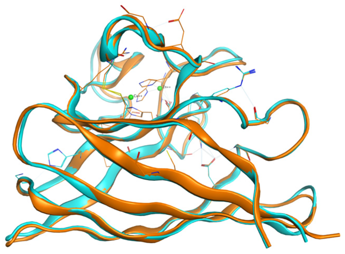
2.1. Structure of the Human Wild-Type Holo Protein
2.2. Mutant Monomer Generation
2.2.1. Mutated Sequences
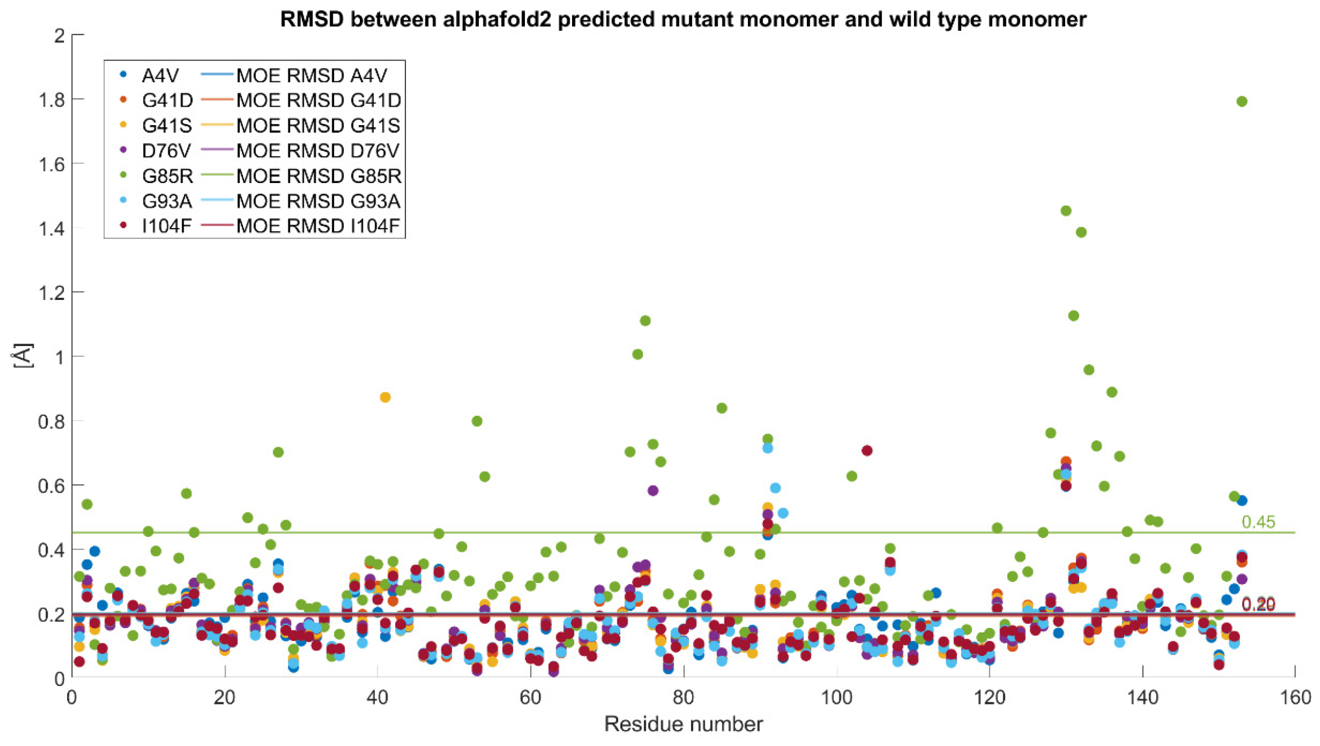
2.2.2. Mutated Structures
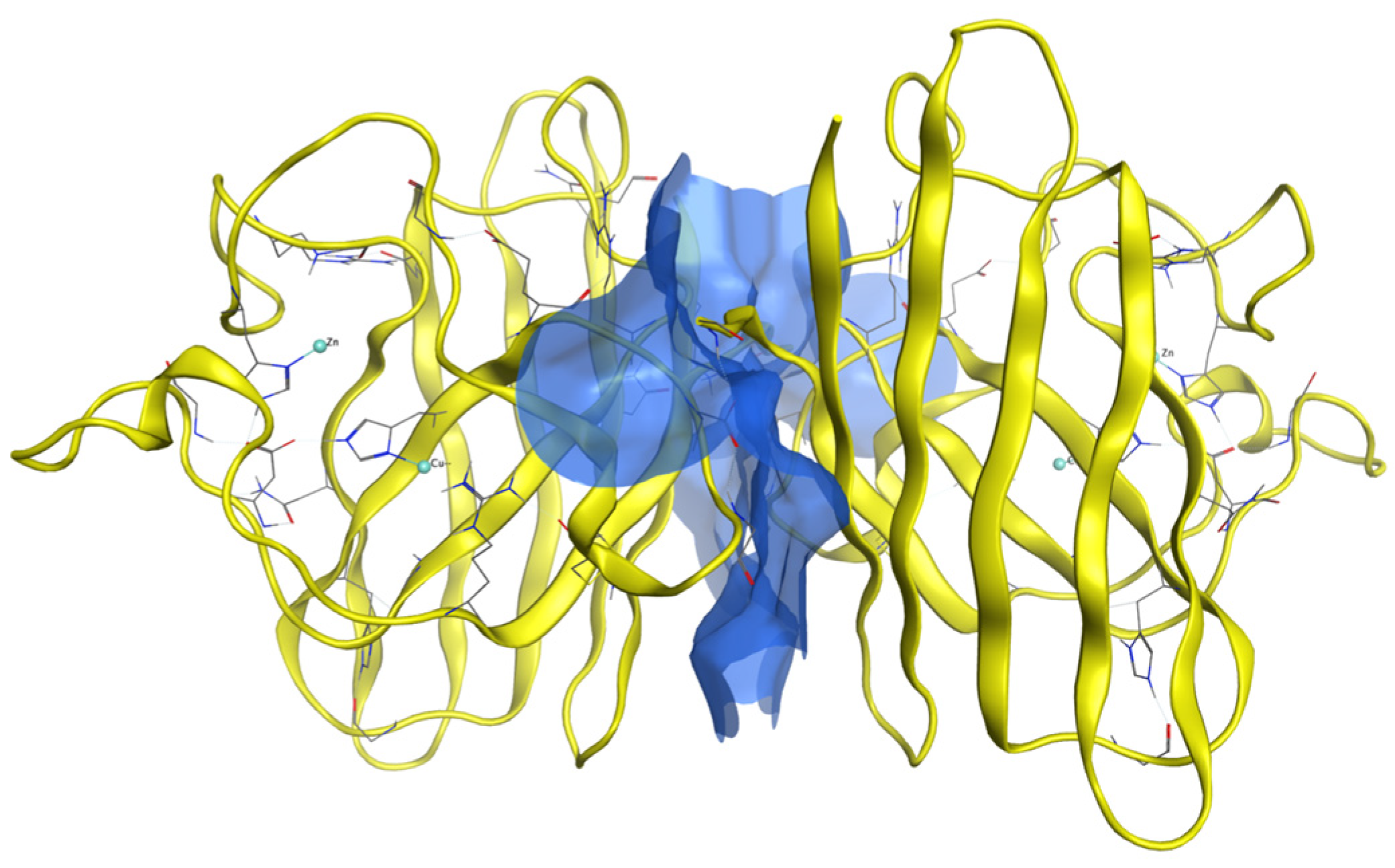
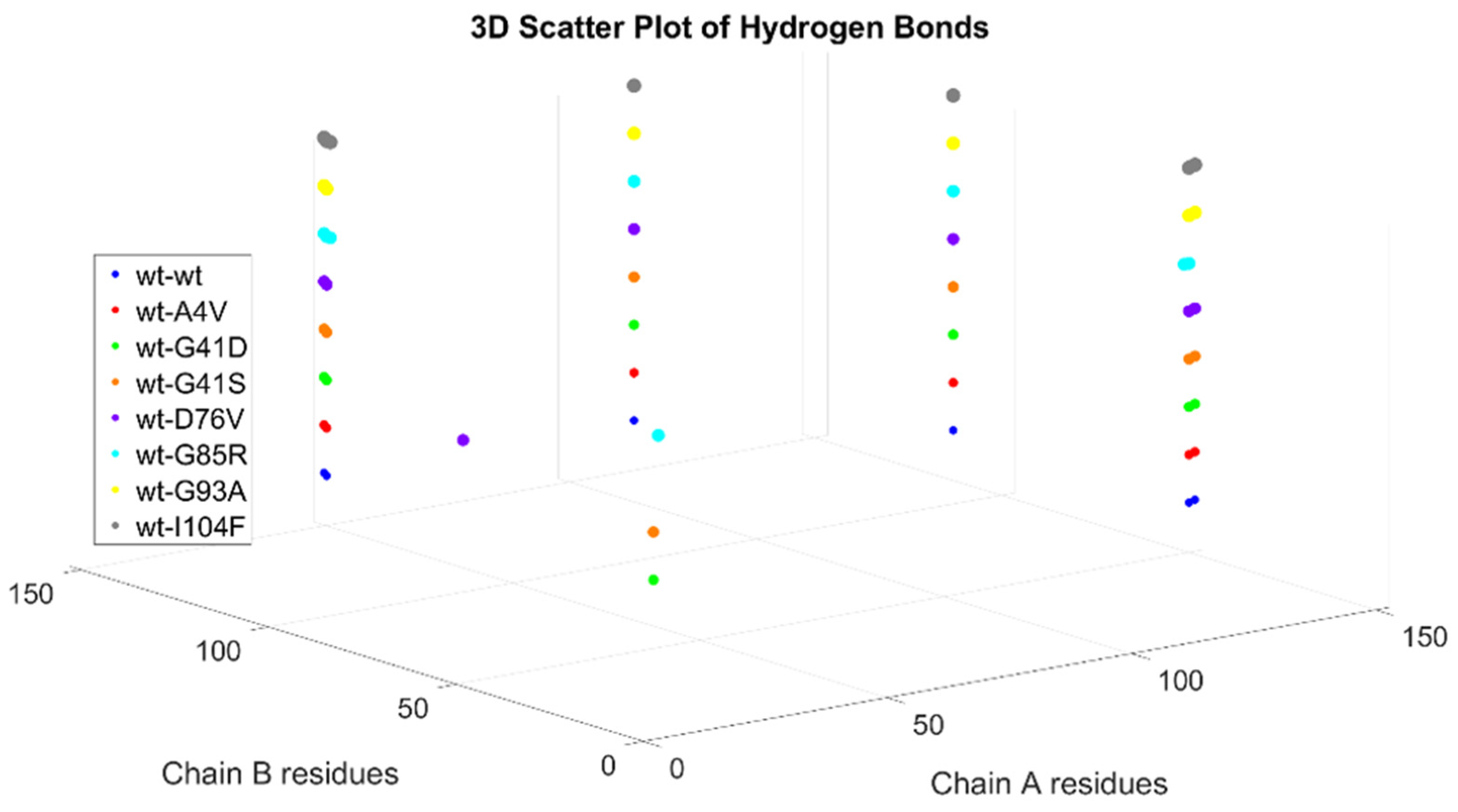
2.3. Generation of Dimers
Dimer Interface Characteristics
2.4. MD Simulations: Data Analysis
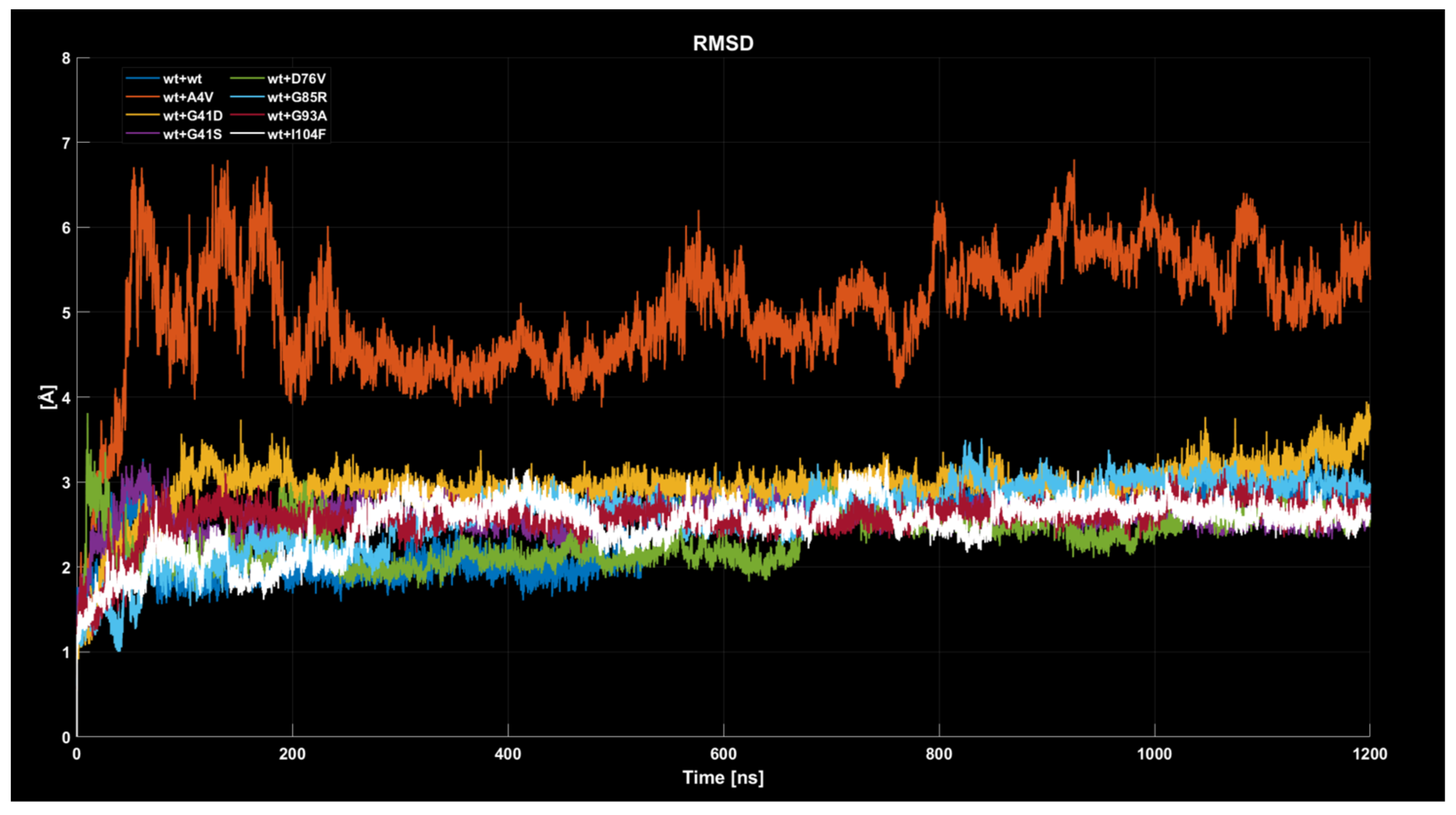
2.4.1. RMSD
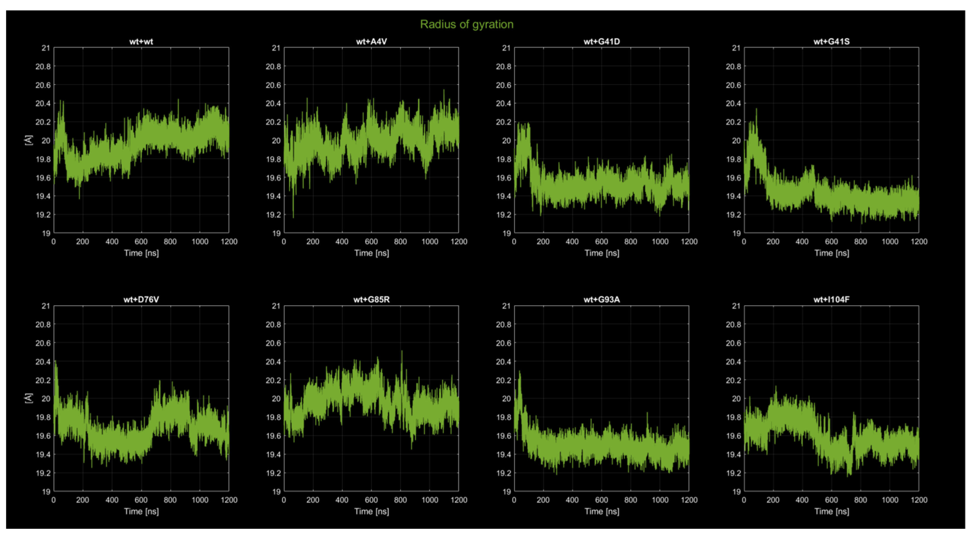
2.4.2. Radius of Gyration
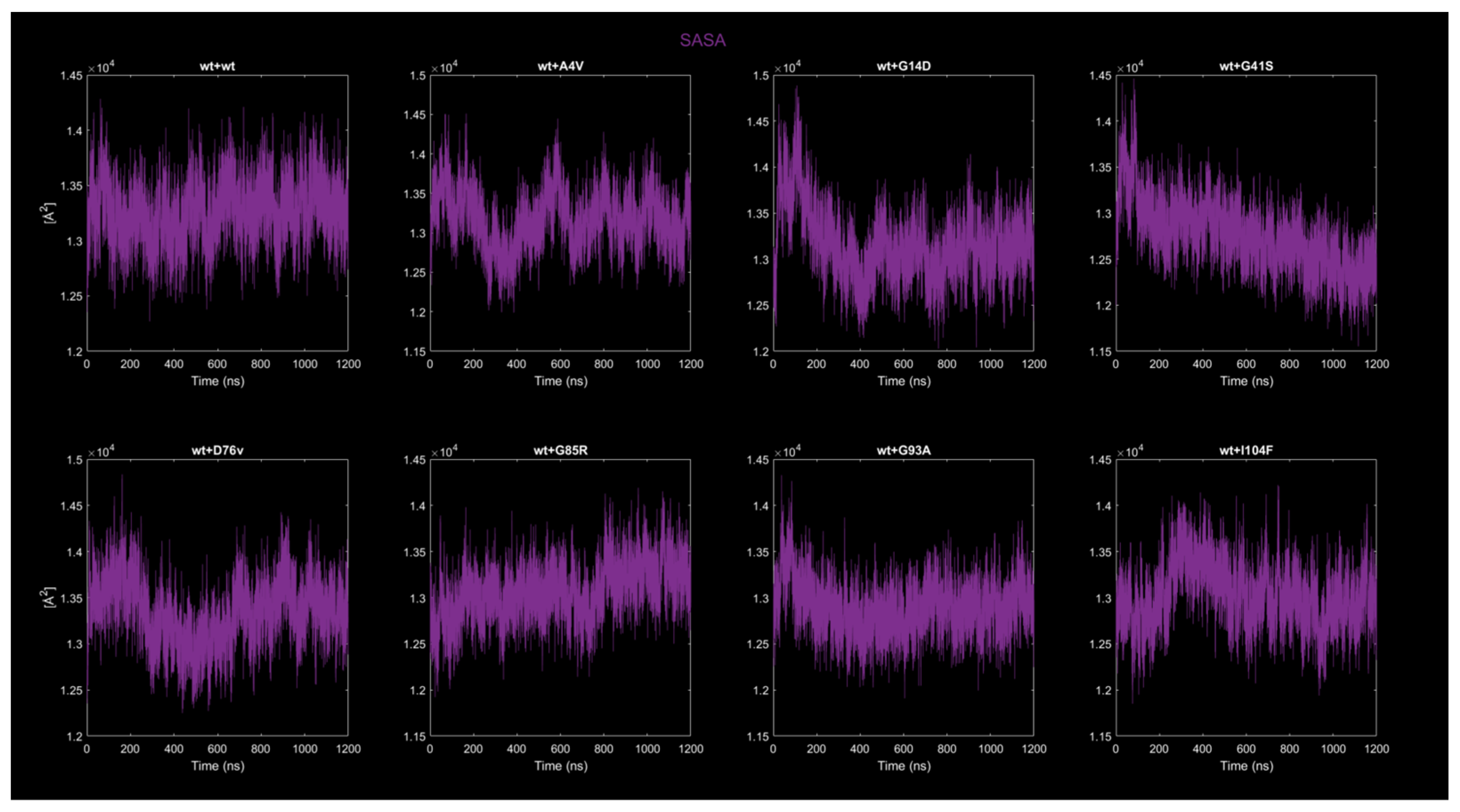
2.4.3. Solvent-Accessible Surface Area (SASA)
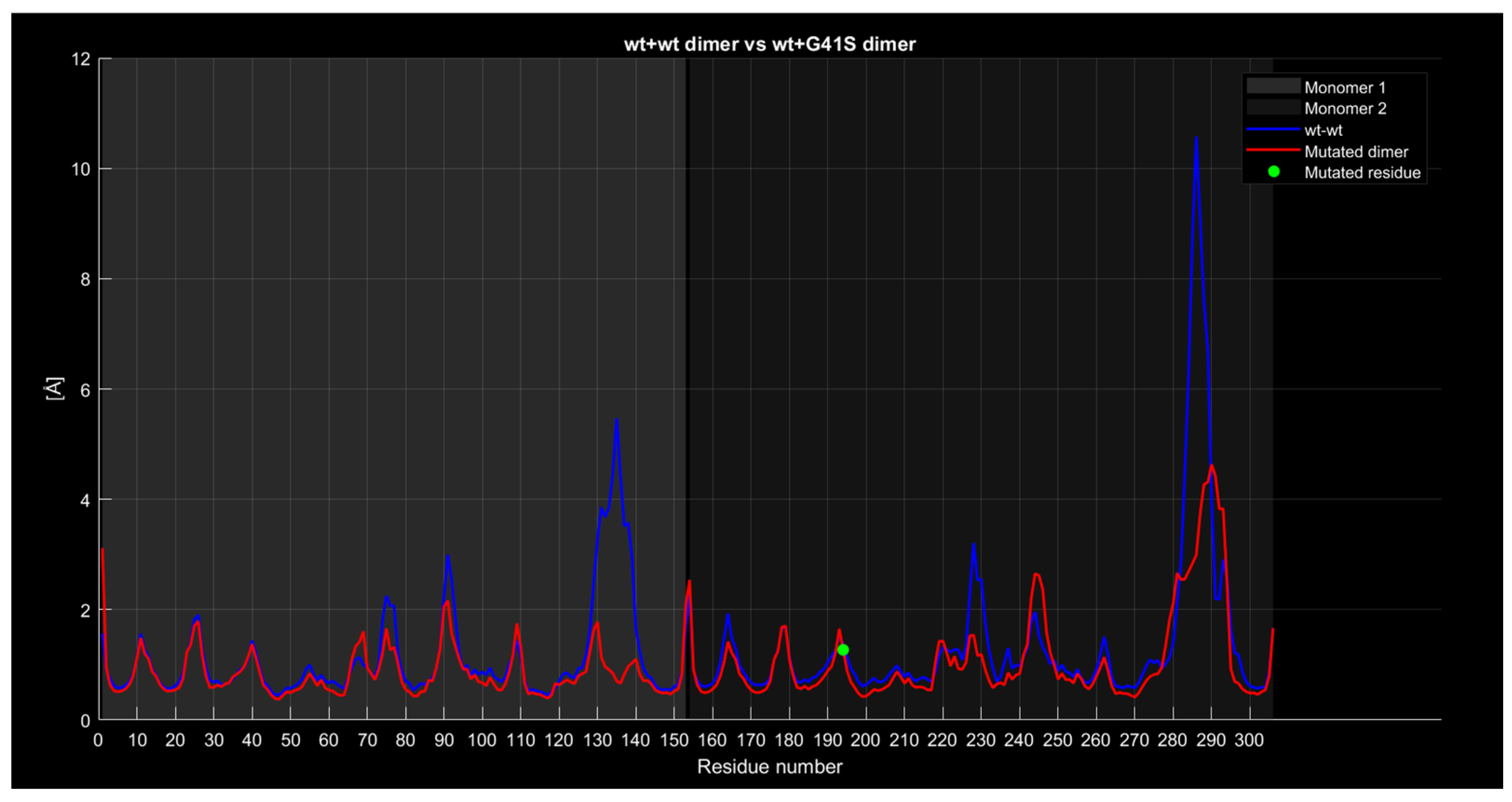
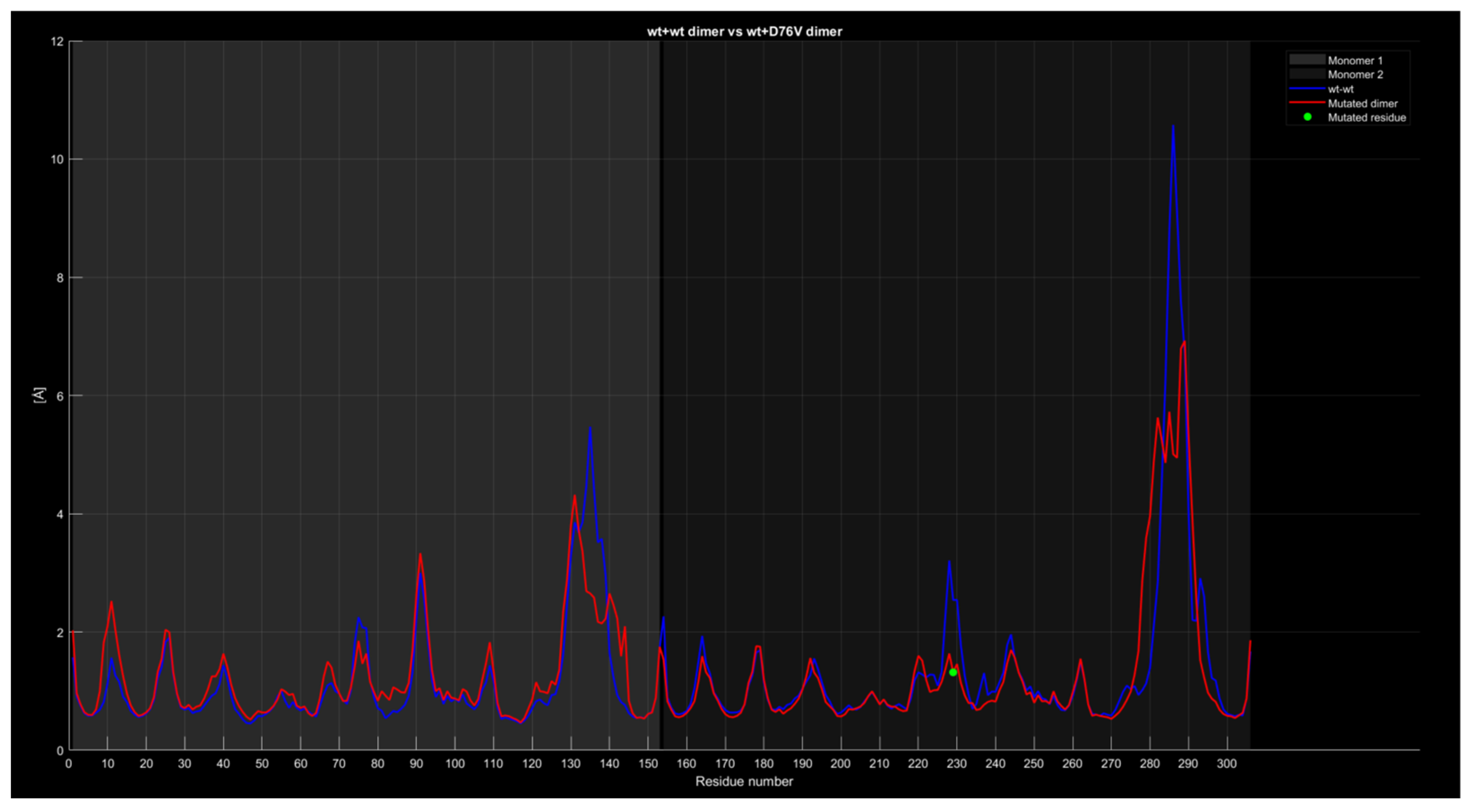
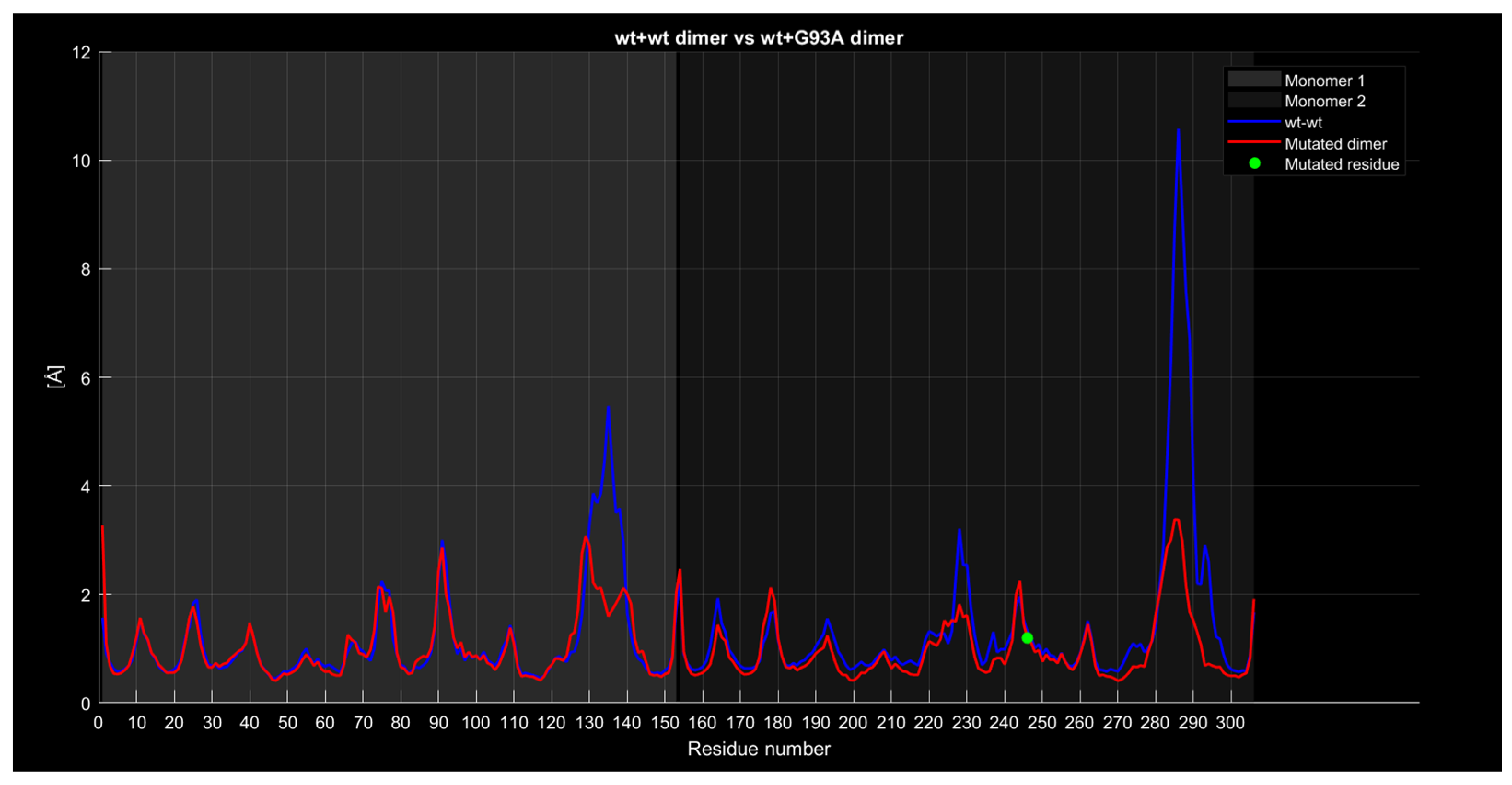
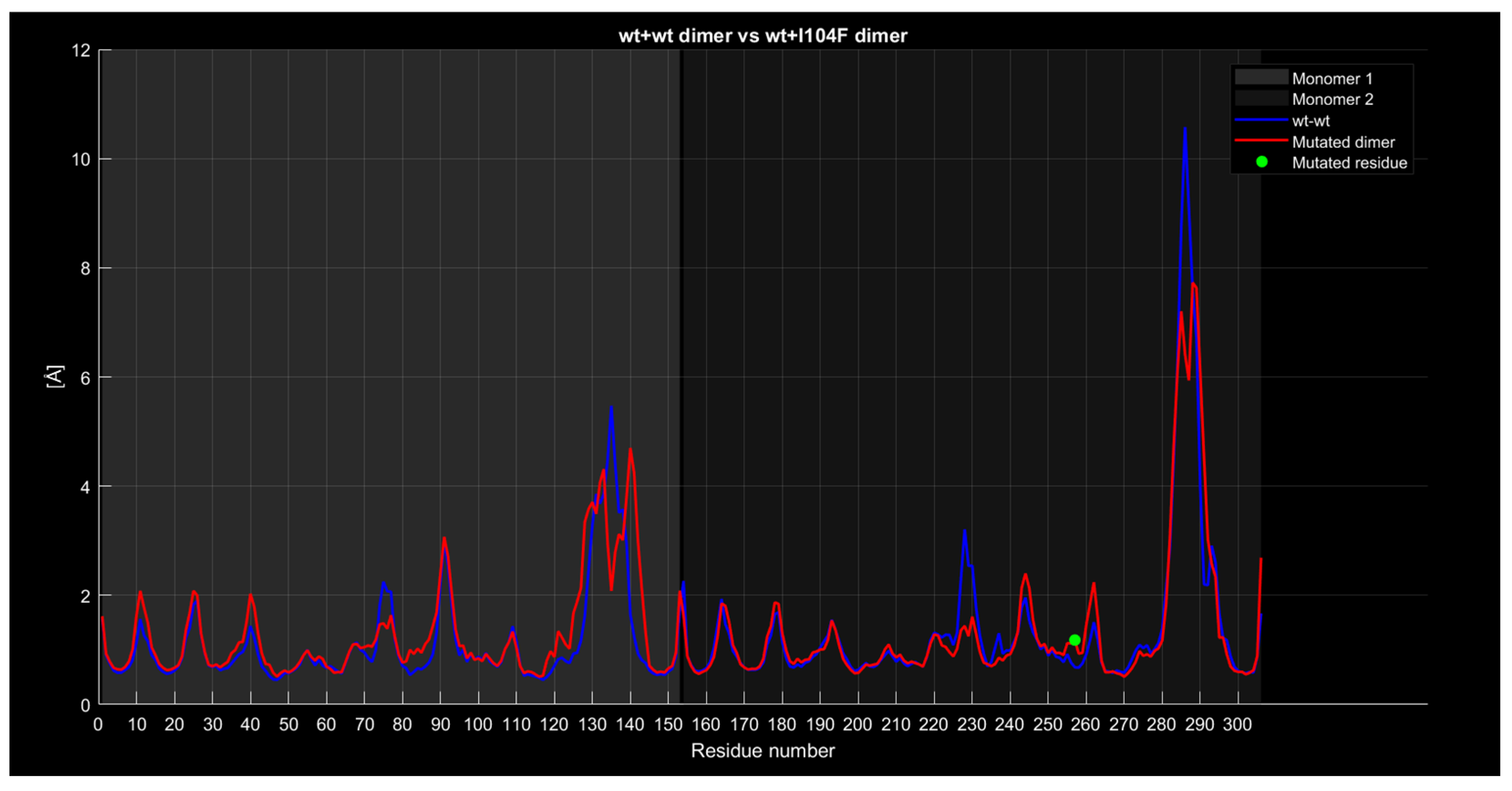
2.4.4. RMSF
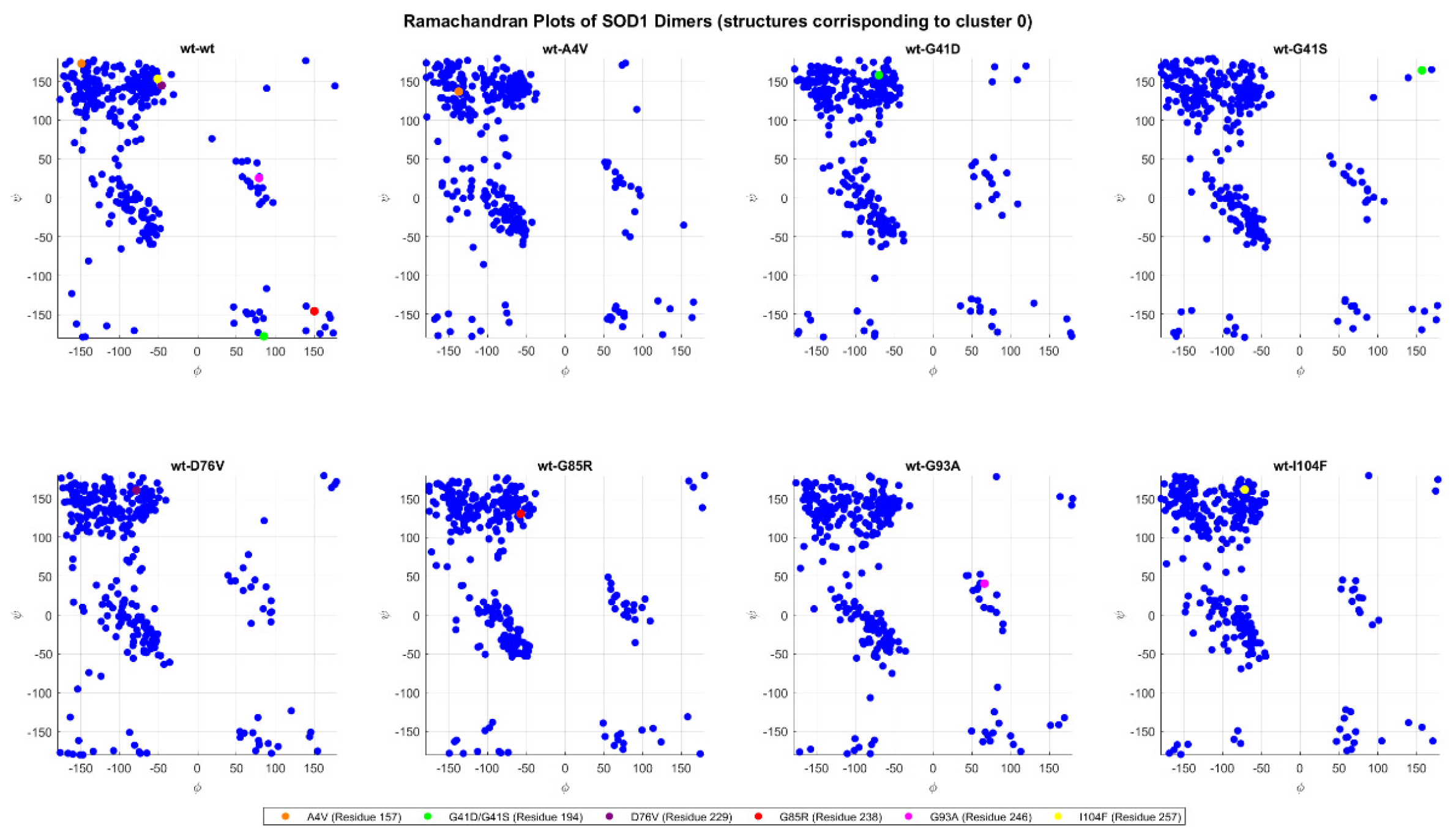
2.4.5. Ramachandran Plots
2.5. Docking Results
Binding Energies and Spatial Pose Clustering Results
3. Discussion
4. Materials and Methods
5. Conclusions
5.1. Best Affinity Ligand Description
5.2. Larger Cluster-Forming Ligand Description
Supplementary Materials
Author Contributions
Funding
Institutional Review Board Statement
Informed Consent Statement
Data Availability Statement
Acknowledgments
Conflicts of Interest
References
- Brotman, R.G.; Moreno-Escobar, M.C.; Joseph, J.; Munakomi, S.; Pawar, G. Amyotrophic Lateral Sclerosis; StatPearls: Treasure Island, FL, USA, 2025. [Google Scholar]
- Rosen, D.R.; Siddique, T.; Patterson, D.; Figlewicz, D.A.; Sapp, P.; Hentati, A.; Donaldson, D.; Goto, J.; O’Regan, J.P.; Deng, H.X.; et al. Mutations in Cu/Zn superoxide dismutase gene are associated with familial amyotrophic lateral sclerosis. Nature 1993, 362, 59–62. [Google Scholar] [CrossRef] [PubMed]
- Berdyński, M.; Miszta, P.; Safranow, K.; Andersen, P.M.; Morita, M.; Filipek, S.; Żekanowski, C.; Kuźma-Kozakiewicz, M. SOD1 mutations associated with amyotrophic lateral sclerosis: Analysis of variant severity. Nature 2022, 12, 103. [Google Scholar] [CrossRef] [PubMed]
- Bernard, E.; Pegat, A.; Svahn, J.; Bouhour, F.; Leblanc, P.; Millecamps, S.; Thobois, S.; Guissart, C.; Lumbroso, S.; Mouzat, K. Clinical and molecular landscape of ALS patients with SOD1 mutations: Novel pathogenic variants and novel phenotypes. A single ALS center study. Int. J. Mol. Sci. 2020, 21, 6807. [Google Scholar] [CrossRef] [PubMed]
- ALSoD. Available online: https://alsod.ac.uk/output/gene.php/SOD1 (accessed on 1 April 2024).
- Hayward, L.J.; Rodriguez, J.A.; Kim, J.W.; Tiwari, A.; Goto, J.J.; Cabelli, D.E.; Selverstone Valentine, J.; Brown, R.H., Jr. Decreased metallation and activity in subsets of mutant superoxide dismutases associated with familial amyotrophic lateral sclerosis. J. Biol. Chem. 2002, 277, 15923–15931. [Google Scholar] [CrossRef]
- Tiwari, A.; Hayward, L.J. Familial amyotrophic lateral sclerosis mutants of copper/zinc superoxide dismutase are susceptible to disulfide reduction. J. Biol. Chem. 2003, 278, 5984–5992. [Google Scholar] [CrossRef]
- Reaume, A.G.; Elliott, J.L.; Hoffman, E.K.; Kowall, N.W.; Ferrante, R.J.; Siwek, D.F.; Wilcox, H.M.; Flood, D.G.; Beal, M.F.; Brown, R.H., Jr.; et al. Motor neurons in Cu/Zn superoxide dismutase-deficient mice develop normally but exhibit enhanced cell death after axonal injury. Nat. Genet. 1996, 13, 43–47. [Google Scholar] [CrossRef]
- Borchelt, D.R.; Lee, M.K.; Slunt, H.S.; Guarnieri, M.; Xu, Z.S.; Wong, P.C.; Brown, R.H., Jr.; Price, D.L.; Sisodia, S.S.; Cleveland, D.W. Superoxide dismutase 1 with mutations linked to familial amyotrophic lateral sclerosis possesses significant activity. Proc. Natl. Acad. Sci. USA 1994, 91, 8292–8296. [Google Scholar] [CrossRef]
- Estévez, A.G.; Crow, J.P.; Sampson, J.B.; Reiter, C.; Zhuang, Y.; Richardson, G.J.; Tarpey, M.M.; Barbeito, L.; Beckman, J.S. Induction of nitric oxide–dependent apoptosis in motor neurons by zinc-deficient superoxide dismutase. Science 1999, 286, 2498–2500. [Google Scholar] [CrossRef]
- Pasinelli, P.; Brown, R.H. Molecular biology of amyotrophic lateral sclerosis: Insights from genetics. Nat. Rev. Neurosci. 2006, 7, 710–723. [Google Scholar] [CrossRef]
- Selverstone Valentine, J.; Doucette, P.A.; Zittin Potter, S. Copper-zinc superoxide dismutase and amyotrophic lateral sclerosis. Annu. Rev. Biochem. 2005, 74, 563–593. [Google Scholar] [CrossRef]
- Nordlund, A.; Oliveberg, M. SOD1-associated ALS: A promising system for elucidating the origin of protein-misfolding disease. HFSP J. 2008, 2, 354–364. [Google Scholar] [CrossRef] [PubMed]
- Chattopadhyay, S.; Uysal, A.; Stripe, B.; Ha, Y.-G.; Marks, T.J.; Karapetrova, E.A.; Dutta, P. How water meets a very hydrophobic surface. Phys. Rev. Lett. 2010, 105, 037803. [Google Scholar] [CrossRef] [PubMed]
- Eisenberg, D.; Jucker, M. The amyloid state of proteins in human diseases. Cell 2012, 148, 1188–1203. [Google Scholar] [CrossRef]
- Guest, W.C. Template-Directed Protein Misfolding in Neurodegenerative Disease; University of British Columbia: Vancouver, BC, Canada, 2012. [Google Scholar]
- Allison, W.T.; DuVal, M.G.; Nguyen-Phuoc, K.; Leighton, P.L.A. Reduced abundance and subverted functions of proteins in prion-like diseases: Gained functions fascinate but lost functions affect aetiology. Int. J. Mol. Sci. 2017, 18, 2223. [Google Scholar] [CrossRef] [PubMed]
- Rodrigo, M.; Ines, M.-G.; Claudio, S. Cross-seeding of misfolded proteins: Implications for etiology and pathogenesis of protein misfolding diseases. PLoS Pathog. 2013, 9, e1003537. [Google Scholar]
- Horwich, A.L.; Weissman, J.S. Deadly conformations—Protein misfolding in prion disease. Cell 1997, 89, 499–510. [Google Scholar] [CrossRef]
- Münch, C.; Bertolotti, A. Exposure of hydrophobic surfaces initiates aggregation of diverse ALS-causing superoxide dismutase-1 mutants. J. Mol. Biol. 2010, 399, 512–525. [Google Scholar] [CrossRef]
- Prusiner, S.B. Prions. Proc. Natl. Acad. Sci. USA 1998, 95, 13363–13383. [Google Scholar] [CrossRef]
- McAlary, L.; Plotkin, S.S.; Yerbury, J.J.; Cashman, N.R. Prion-like propagation of protein misfolding and aggregation in amyotrophic lateral sclerosis. Front. Neurosci. 2019, 12, 4–7. [Google Scholar] [CrossRef]
- Hamzeh, B. Probing the Effects of Pathogenic Mutations on Prion-like Conversion of Superoxide Dismutase-1. Master’s Thesis, University of Alberta, Edmonton, AB, Canada, 2024. [Google Scholar]
- Keerthana, S.P.; Kolandaivel, P. Interaction between dimer interface residues of native and mutated SOD1 protein: A theoretical study. J. Biol. Inorg. Chem. 2015, 20, 509–522. [Google Scholar] [CrossRef]
- Molecular Operating Environment (MOE). 2024.0601; Chemical Computing Group ULC: Montreal, QC, Canada, 2025; Available online: https://www.chemcomp.com/en/Products.htm (accessed on 10 May 2024).
- The MathWorks Inc. MATLAB, Version: 9.13.0 (R2022b). The MathWorks Inc.: Natick, MA, USA, 2022; Available online: https://www.mathworks.com (accessed on 10 May 2024).
- Jumper, J.; Evans, R.; Pritzel, A.; Green, T.; Figurnov, M.; Ronneberger, O.; Tunyasuvunakool, K.; Bates, R.; Žídek, A.; Potapenko, A.; et al. Highly accurate protein structure prediction with AlphaFold. Nature 2021, 596, 583–589. [Google Scholar] [CrossRef] [PubMed]
- Dominguez, C.; Boelens, R.; Bonvin, A.M.J.J. HADDOCK: A protein-protein docking approach based on biochemical and/or biophysical information. J. Am. Chem. Soc. 2003, 125, 1731–1737. [Google Scholar] [CrossRef]
- Van Zundert, G.C.P.; Rodrigues, J.P.G.L.M.; Trellet, M.; Schmitz, C.; Kastritis, P.L.; Karaca, E.; Melquiond, A.S.J.; van Dijk, M.; De Vries, S.J.; Bonvin, A.M.J.J. The HADDOCK2.2 webserver: User-friendly integrative modeling of biomolecular complexes. J. Mol. Biol. 2016, 428, 720–725. [Google Scholar] [CrossRef] [PubMed]
- Rodrigues, J.P.G.L.M.; Teixeira, J.M.C.; Trellet, M.; Bonvin, A.M.J.J. pdb-tools: A swiss army knife for molecular structures. F1000Research 2018, 7, 1961. [Google Scholar] [CrossRef]
- Case, D.A.; Aktulga, H.M.; Belfon, K.; Ben-Shalom, I.Y.; Berryman, J.T.; Brozell, S.R.; Cerutti, D.S.; Cheatham, T.E., III; Cisneros, G.A.; Cruzeiro, V.W.D.; et al. Amber 2024; University of California: San Francisco, CA, USA, 2024. [Google Scholar]
- Case, D.A.; Aktulga, H.M.; Belfon, K.; Cerutti, D.S.; Cisneros, G.A.; Cruzeiro, V.W.D.; Forouzesh, N.; Giese, T.J.; Götz, A.W.; Gohlke, H.; et al. AmberTools. J. Chem. Inf. Model. 2023, 63, 6183–6191. [Google Scholar] [CrossRef] [PubMed]
- Woo, T.-G.; Yoon, M.-H.; Kang, S.-M.; Park, S.; Cho, J.-H.; Hwang, Y.J.; Ahn, J.; Jang, H.; Shin, Y.-J.; Jung, E.-M.; et al. Novel chemical inhibitor against SOD1 misfolding and aggregation protects neuron-loss and ameliorates disease symptoms in ALS mouse model. Commun. Biol. 2021, 4, 1397. [Google Scholar] [CrossRef]
- DuVal, M.G.; Hinge, V.K.; Snyder, N.; Kanyo, R.; Bratvold, J.; Pokrishevsky, E.; Cashman, N.R.; Blinov, N.; Kovalenko, A.; Allison, W.T. Tryptophan 32 mediates SOD1 toxicity in an in vivo motor neuron model of ALS and is a promising target for small molecule therapeutics. Neurobiol. Dis. 2019, 124, 297–310. [Google Scholar] [CrossRef]
- Hossain, M.A.; Sarin, R.; Donnelly, D.P.; Miller, B.C.; Weiss, A.; McAlary, L.; Antonyuk, S.V.; Salisbury, J.P.; Amin, J.; Conway, J.B.; et al. Evaluating protein cross-linking as a therapeutic strategy to stabilize SOD1 variants in a mouse model of familial ALS. PLoS Biol. 2024, 22, e3002462. [Google Scholar] [CrossRef]
- Knox, C.; Wilson, M.; Klinger, C.M.; Franklin, M.; Oler, E.; Wilson, A.; Pon, A.; Cox, J.; Chin, N.E.; A Strawbridge, S.; et al. DrugBank 6.0: The DrugBank Knowledgebase for 2024. Nucleic Acids Res. 2024, 52, D1265–D1275. [Google Scholar] [CrossRef]
- Eberhardt, J.; Santos-Martins, D.; Tillack, A.F.; Forli, S. AutoDock Vina 1.2.0: New Docking Methods, Expanded Force Field, and Python Bindings. J. Chem. Inf. Model. 2021, 61, 3891–3898. [Google Scholar] [CrossRef]
- Trott, O.; Olson, A.J. AutoDock Vina: Improving the speed and accuracy of docking with a new scoring function, efficient optimization, and multithreading. J. Comput. Chem. 2010, 31, 455–461. [Google Scholar] [CrossRef] [PubMed]
- Schmidlin, T.; Kennedy, B.K.; Daggett, V. Structural Changes to Monomeric CuZn Superoxide Dismutase Caused by the Familial Amyotrophic Lateral Sclerosis-Associated Mutation A4V. Biophys. J. 2009, 97, 1709–1718. [Google Scholar] [CrossRef] [PubMed]


| Monomer | Sequence |
|---|---|
| wt | ATKAVCVLKGDGPVQGIINFEQKESNGPVKVWGSIKGLTEGLHGFHVHEFGDNTAGCTSAGPHFNPLSRKHGGPKDEERHVGDLGNVTADKDGVADVSIEDSVISLSGDHCIIGRTLVVHEKADDLGKGGNEESTKTGNAGSRLACGVIGIAQ |
| A4V | ATKVVCVLKGDGPVQGIINFEQKESNGPVKVWGSIKGLTEGLHGFHVHEFGDNTAGCTSAGPHFNPLSRKHGGPKDEERHVGDLGNVTADKDGVADVSIEDSVISLSGDHCIIGRTLVVHEKADDLGKGGNEESTKTGNAGSRLACGVIGIAQ |
| G41D | ATKAVCVLKGDGPVQGIINFEQKESNGPVKVWGSIKGLTEDLHGFHVHEFGDNTAGCTSAGPHFNPLSRKHGGPKDEERHVGDLGNVTADKDGVADVSIEDSVISLSGDHCIIGRTLVVHEKADDLGKGGNEESTKTGNAGSRLACGVIGIAQ |
| G41S | ATKAVCVLKGDGPVQGIINFEQKESNGPVKVWGSIKGLTESLHGFHVHEFGDNTAGCTSAGPHFNPLSRKHGGPKDEERHVGDLGNVTADKDGVADVSIEDSVISLSGDHCIIGRTLVVHEKADDLGKGGNEESTKTGNAGSRLACGVIGIAQ |
| D76V | ATKAVCVLKGDGPVQGIINFEQKESNGPVKVWGSIKGLTEGLHGFHVHEFGDNTAGCTSAGPHFNPLSRKHGGPKVEERHVGDLGNVTADKDGVADVSIEDSVISLSGDHCIIGRTLVVHEKADDLGKGGNEESTKTGNAGSRLACGVIGIAQ |
| G85R | ATKAVCVLKGDGPVQGIINFEQKESNGPVKVWGSIKGLTEGLHGFHVHEFGDNTAGCTSAGPHFNPLSRKHGGPKDEERHVGDLRNVTADKDGVADVSIEDSVISLSGDHCIIGRTLVVHEKADDLGKGGNEESTKTGNAGSRLACGVIGIAQ |
| G93A | ATKAVCVLKGDGPVQGIINFEQKESNGPVKVWGSIKGLTEGLHGFHVHEFGDNTAGCTSAGPHFNPLSRKHGGPKDEERHVGDLGNVTADKDAVADVSIEDSVISLSGDHCIIGRTLVVHEKADDLGKGGNEESTKTGNAGSRLACGVIGIAQ |
| I104F | ATKAVCVLKGDGPVQGIINFEQKESNGPVKVWGSIKGLTEGLHGFHVHEFGDNTAGCTSAGPHFNPLSRKHGGPKDEERHVGDLGNVTADKDGVADVSIEDSVFSLSGDHCIIGRTLVVHEKADDLGKGGNEESTKTGNAGSRLACGVIGIAQ |
| Ligand 22 | ||
|---|---|---|
| Iteration 1 model 1 | Iteration 2 model 1 | Iteration 3 model 1 |
 |  |  |
| Iteration 4 model 1 | Iteration 5 model 1 | Iteration 6 model 1 |
 |  |  |
| Iteration 7 model 1 | Iteration 8 model 1 | Iteration 9 model 1 |
 |  |  |
| Iteration 10 model 1 | ||
 | ||
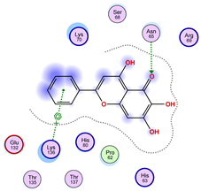
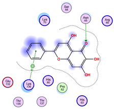
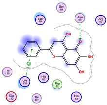
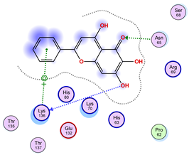
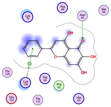
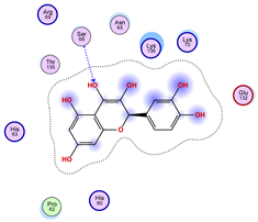
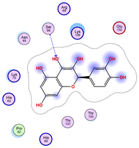
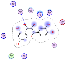
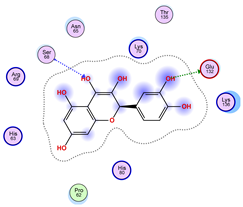
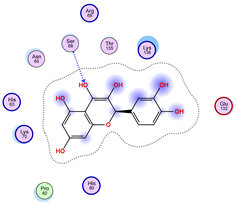
| Ligand 36 | ||
|---|---|---|
| Iteration 1 model 1 | Iteration 2 model 1 | Iteration 3 model 1 |
 |  |  |
| Iteration 4 model 1 | Iteration 5 model 1 | Iteration 6 model 1 |
 |  |  |
| Iteration 7 model 1 | Iteration 8 model 1 | Iteration 9 model 1 |
 | 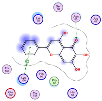 |  |
| Iteration 10 model 1 | ||
 | ||
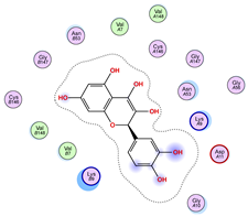
| Ligand 38 | ||
|---|---|---|
| Iteration 1 model 1 | Iteration 2 model 1 | Iteration 3 model 1 |
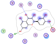 | 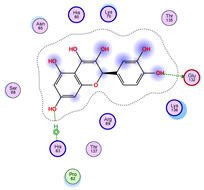 |  |
| Iteration 4 model 1 | Iteration 5 model 1 | Iteration 6 model 1 |
 |  |  |
| Iteration 7 model 1 | Iteration 8 model 1 | Iteration 9 model 1 |
 |  |  |
| Iteration 10 model 1 | ||
 | ||
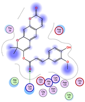
| Model | Atom Ligand (ID) | Atom Receptor | Res. Receptor | Chain (Monomer) | Interaction Type | Distance (Å) | E (kcal/mol) |
|---|---|---|---|---|---|---|---|
| Iteration 1 | |||||||
| 1 | O27 (20) | NZ | LYS 122 | B | H-acceptor | 3.08 | −1.8 |
| 2 | C31 (17) | OE2 | GLU 49 | B | H-donor | 3.59 | −0.6 |
| 3 | — | — | — | — | — | — | — |
| 4 | O27 (20) | NZ | LYS 122 | A | H-acceptor | 3.38 | −0.9 |
| 5 | — | — | — | — | — | — | — |
| 6 | O15 (18) | NE | ARG 143 | B | H-acceptor | 3.16 | −0.6 |
| 6-ring | CA | GLY 141 | B | pi-H | 3.94 | −0.5 | |
| 7 | C25 (30) | OG1 | THR 137 | B | H-donor | 3.30 | −0.6 |
| O27 (20) | CA | PRO 62 | B | H-acceptor | 3.37 | −1.1 | |
| 8 | C25 (30) | SG | CYS 111 | B | H-donor | 3.71 | −0.7 |
| 9 | C25 (30) | OD1 | ASN 139 | B | H-donor | 3.55 | −0.7 |
| O6 (6) | ND2 | ASN 65 | B | H-acceptor | 2.95 | −1.6 | |
| 10 | O6 (6) | NE2 | GLN 153 | A | H-acceptor | 3.21 | −0.7 |
| Iteration 2 | |||||||
| Model | Atom Ligand (ID) | Atom Receptor | Res. Receptor | Chain (monomer) | Interaction type | Distance (Å) | E (kcal/mol) |
| 1 | O6 (6) | NE2 | GLN 153 | A | H-acceptor | 3.13 | −1.3 |
| 6-ring | CA | GLY 61 | B | pi-H | 3.61 | −2.4 | |
| 2 | 6-ring | CA | GLY 61 | A | pi-H | 3.36 | −0.8 |
| 3 | O27 (20) | NZ | LYS 122 | A | H-acceptor | 3.18 | −1.8 |
| 4 | — | — | — | — | — | — | — |
| 5 | C31 (17) | OE2 | GLU 49 | B | H-donor | 3.28 | −0.7 |
| 6 | — | — | — | — | — | — | — |
| 7 | O6 (6) | NE1 | TRP 32 | B | H-acceptor | 3.23 | −0.6 |
| 8 | O26 (31) | OD2 | ASP 11 | B | H-donor | 3.14 | −0.8 |
| 6-ring | NZ | LYS 36 | A | pi-cation | 4.22 | −0.9 | |
| 9 | C3 (3) | OE2 | GLU 49 | B | H-donor | 3.49 | −1.5 |
| C30 (16) | O | ARG 69 | B | H-donor | 3.68 | −0.5 | |
| O27 (20) | N | HIS 63 | B | H-acceptor | 3.24 | −1.2 | |
| 10 | C3 (3) | OE2 | GLU 49 | B | H-donor | 3.69 | −1.1 |
| O27 (20) | CE1 | HIS 80 | B | H-acceptor | 3.66 | −0.5 | |
| Iteration 3 | |||||||
| Model | Atom Ligand (ID) | Atom Receptor | Res. Receptor | Chain (monomer) | Interaction type | Distance (Å) | E (kcal/mol) |
| 1 | O27 (20) | NZ | LYS 122 | A | H-acceptor | 3.17 | −1.5 |
| 6-ring | CA | ASP 125 | A | pi-H | 3.64 | −0.6 | |
| 2 | O26 (31) | O | GLU 40 | B | H-donor | 2.89 | −1.4 |
| O27 (20) | NZ | LYS 122 | B | H-acceptor | 3.19 | −1.1 | |
| 3 | O27 (20) | CA | PRO 66 | A | H-acceptor | 3.57 | −0.5 |
| O24 (29) | NH2 | ARG 115 | A | H-acceptor | 3.10 | −1.4 | |
| 4 | — | — | — | — | — | — | — |
| 5 | C25 (30) | O | ASP 109 | B | H-donor | 3.77 | −0.5 |
| O27 (20) | CA | PRO 66 | B | H-acceptor | 3.64 | −0.5 | |
| 6 | O27 (20) | CA | PRO 62 | A | H-acceptor | 3.35 | −1.1 |
| 6-ring | CG | LYS 136 | A | pi-H | 3.64 | −0.5 | |
| 7 | C7 (7) | OG1 | THR 137 | B | H-donor | 3.52 | −0.6 |
| 6-ring | CA | GLY 141 | B | pi-H | 3.78 | −0.5 | |
| 8 | O6 (6) | NE1 | TRP 32 | B | H-acceptor | 3.07 | −1.8 |
| 9 | — | — | — | — | — | — | — |
| 10 | O24 (29) | ND2 | ASN 65 | A | H-acceptor | 3.02 | −1.5 |
| Iteration 4 | |||||||
| Model | Atom Ligand (ID) | Atom Receptor | Res. Receptor | Chain (monomer) | Interaction type | Distance (Å) | E (kcal/mol) |
| 1 | C25 (30) | O | HIS 63 | B | H-donor | 3.70 | −0.5 |
| O6 (6) | NE2 | GLN 153 | A | H-acceptor | 3.24 | −0.8 | |
| 6-ring | CA | GLY 61 | B | pi-H | 3.66 | −1.8 | |
| 2 | C25 (30) | O | HIS 63 | A | H-donor | 3.65 | −0.7 |
| O6 (6) | NE2 | GLN 153 | B | H-acceptor | 3.23 | −1.6 | |
| 3 | C8 (8) | O | ILE 17 | B | H-donor | 3.32 | −0.5 |
| C12 (12) | O | SER 34 | B | H-donor | 3.58 | −0.5 | |
| 4 | C25 (30) | O | ASP 92 | A | H-donor | 3.48 | −0.8 |
| 5 | C31 (17) | OE2 | GLU 49 | B | H-donor | 3.51 | −0.5 |
| 6 | C25 (30) | OG1 | THR 137 | A | H-donor | 3.45 | −0.6 |
| O27 (20) | CA | PRO 62 | A | H-acceptor | 3.51 | −0.8 | |
| 6-ring | CG | LYS 136 | A | pi-H | 3.68 | −0.5 | |
| 7 | O6 (6) | CA | GLY 33 | B | H-acceptor | 3.65 | −0.7 |
| O27 (20) | NZ | LYS 36 | B | H-acceptor | 2.98 | −2.7 | |
| 8 | C3 (3) | O | HIS 63 | B | H-donor | 3.55 | −0.7 |
| C8 (8) | O | HIS 63 | B | H-donor | 3.66 | −0.5 | |
| C25 (30) | O | ASP 109 | B | H-donor | 3.53 | −0.7 | |
| O27 (20) | CA | PRO 66 | B | H-acceptor | 3.50 | −0.6 | |
| 9 | C25 (30) | OE1 | GLN 153 | A | H-donor | 3.33 | −0.5 |
| 6-ring | CA | GLY 61 | B | pi-H | 3.80 | −1.0 | |
| 10 | O27 (20) | CA | PRO 62 | B | H-acceptor | 3.61 | −0.7 |
| Iteration 5 | |||||||
| Model | Atom Ligand (ID) | Atom Receptor | Res. Receptor | Chain (monomer) | Interaction type | Distance (Å) | E (kcal/mol) |
| 1 | C25 (30) | O | HIS 63 | B | H-donor | 3.71 | −0.6 |
| O6 (6) | NE2 | GLN 153 | A | H-acceptor | 3.11 | −1.6 | |
| 6-ring | CA | GLY 61 | B | pi-H | 3.67 | −0.6 | |
| 2 | O27 (20) | NZ | LYS 122 | B | H-acceptor | 3.21 | −1.2 |
| 6-ring | CA | ASP 125 | B | pi-H | 3.68 | −0.7 | |
| 3 | O27 (20) | NZ | LYS 122 | A | H-acceptor | 3.07 | −2.0 |
| 4 | O6 (6) | NE2 | GLN 153 | B | H-acceptor | 3.08 | −1.9 |
| O27 (20) | CD | LYS 136 | A | H-acceptor | 3.58 | −0.5 | |
| 5 | C31 (17) | OE1 | GLU 49 | A | H-donor | 3.55 | −0.5 |
| 6 | — | — | — | — | — | — | — |
| 7 | C8 (8) | O | HIS 63 | B | H-donor | 3.51 | −0.5 |
| O27 (20) | CA | PRO 66 | B | H-acceptor | 3.57 | −0.5 | |
| 8 | — | — | — | — | — | — | — |
| 9 | C8 (8) | O | ILE 17 | B | H-donor | 3.12 | −0.6 |
| C12 (12) | O | SER 34 | B | H-donor | 3.46 | −0.6 | |
| 10 | O6 (6) | ND2 | ASN 53 | B | H-acceptor | 3.12 | −2.4 |
| Iteration 6 | |||||||
| Model | Atom Ligand (ID) | Atom Receptor | Res. Receptor | Chain (monomer) | Interaction type | Distance (Å) | E (kcal/mol) |
| 1 | O27 (20) | NZ | LYS 122 | A | H-acceptor | 3.17 | −1.5 |
| O24 (29) | OG1 | THR 39 | A | H-acceptor | 2.84 | −1.1 | |
| 6-ring | CA | ASP 125 | A | pi-H | 3.68 | −0.7 | |
| 2 | C25 (30) | O | HIS 63 | A | H-donor | 3.82 | −0.6 |
| 6-ring | CA | GLY 61 | A | pi-H | 3.56 | −1.1 | |
| 3 | O27 (20) | NZ | LYS 122 | B | H-acceptor | 3.12 | −1.6 |
| O24 (29) | OG1 | THR 39 | B | H-acceptor | 2.87 | −0.9 | |
| 4 | — | — | — | — | — | — | — |
| 5 | — | — | — | — | — | — | — |
| 6 | O6 (6) | NE2 | GLN 153 | A | H-acceptor | 2.99 | −3.0 |
| 7 | — | — | — | — | — | — | — |
| 8 | O27 (20) | CA | PRO 66 | B | H-acceptor | 3.47 | −0.7 |
| 9 | C3 (3) | O | HIS 63 | A | H-donor | 3.46 | −0.6 |
| 10 | C25 (30) | OD1 | ASN 139 | B | H-donor | 3.70 | −0.5 |
| O6 (6) | ND2 | ASN 65 | B | H-acceptor | 2.93 | −2.1 | |
| Iteration 7 | |||||||
| Model | Atom Ligand (ID) | Atom Receptor | Res. Receptor | Chain (monomer) | Interaction type | Distance (Å) | E (kcal/mol) |
| 1 | O26 (31) | O | ARG 69 | B | H-donor | 2.88 | −0.7 |
| O6 (6) | NE2 | GLN 153 | A | H-acceptor | 3.27 | −0.6 | |
| 6-ring | CA | GLY 61 | B | pi-H | 3.57 | −1.6 | |
| 2 | C25 (30) | O | HIS 63 | A | H-donor | 3.59 | −0.7 |
| 6-ring | CA | GLY 61 | A | pi-H | 3.38 | −1.0 | |
| 3 | O27 (20) | NZ | LYS 122 | A | H-acceptor | 3.20 | −1.7 |
| 4 | C25 (30) | O | ASP 92 | A | H-donor | 3.83 | −0.5 |
| 5 | — | — | — | — | — | — | — |
| 6 | 6-ring | 6-ring | TRP 32 | A | pi-pi | 3.69 | −0.0 |
| 6-ring | 5-ring | TRP 32 | A | pi-pi | 3.62 | −0.0 | |
| 7 | C7 (7) | OG1 | THR 137 | B | H-donor | 3.48 | −0.6 |
| C25 (30) | O | ARG 143 | B | H-donor | 3.43 | −0.5 | |
| 6-ring | CA | GLY 141 | B | pi-H | 3.70 | −0.5 | |
| 6-ring | N | ARG 143 | B | pi-H | 4.20 | −0.6 | |
| 8 | C25 (30) | O | HIS 63 | A | H-donor | 3.67 | −0.7 |
| 9 | — | — | — | — | — | — | — |
| 10 | — | — | — | — | — | — | — |
| Iteration 8 | |||||||
| Model | Atom Ligand (ID) | Atom Receptor | Res. Receptor | Chain (monomer) | Interaction type | Distance (Å) | E (kcal/mol) |
| 1 | C31 (17) | OE1 | GLU 49 | A | H-donor | 3.47 | −0.5 |
| 2 | O27 (20) | CE | LYS 122 | A | H-acceptor | 3.46 | −1.3 |
| 3 | O27 (20) | NZ | LYS 122 | B | H-acceptor | 3.23 | −1.0 |
| 4 | C25 (30) | O | ASP 92 | A | H-donor | 3.71 | −0.6 |
| 5 | 6-ring | 6-ring | TRP 32 | A | pi-pi | 3.70 | −0.0 |
| 6-ring | 5-ring | TRP 32 | A | pi-pi | 3.62 | −0.0 | |
| 6 | O27 (20) | CA | PRO 62 | B | H-acceptor | 3.44 | −0.9 |
| 6-ring | CG | LYS 136 | B | pi-H | 3.61 | −0.5 | |
| 7 | — | — | — | — | — | — | — |
| 8 | O15 (18) | NH2 | ARG 143 | B | H-acceptor | 2.94 | −1.3 |
| 9 | O6 (6) | NZ | LYS 9 | B | H-acceptor | 3.25 | −2.1 |
| 10 | — | — | — | — | — | — | — |
| Iteration 9 | |||||||
| Model | Atom Ligand (ID) | Atom Receptor | Res. Receptor | Chain (monomer) | Interaction type | Distance (Å) | E (kcal/mol) |
| 1 | C25 (30) | O | HIS 63 | A | H-donor | 3.57 | −0.7 |
| O26 (31) | O | ARG 69 | A | H-donor | 2.73 | −1.3 | |
| O6 (6) | NE2 | GLN 153 | B | H-acceptor | 3.22 | −1.4 | |
| O27 (20) | CD | LYS 136 | A | H-acceptor | 3.56 | −0.5 | |
| 6-ring | CA | GLY 61 | A | pi-H | 3.82 | −0.6 | |
| 2 | C25 (30) | O | HIS 63 | B | H-donor | 3.64 | −0.7 |
| O6 (6) | NE2 | GLN 153 | A | H-acceptor | 2.82 | −3.8 | |
| 3 | O27 (20) | CE | LYS 122 | A | H-acceptor | 3.47 | −1.2 |
| 4 | C8 (8) | O | ILE 17 | B | H-donor | 3.18 | −0.6 |
| C12 (12) | O | SER 34 | B | H-donor | 3.49 | −0.6 | |
| 5 | — | — | — | — | — | — | — |
| 6 | C25 (30) | O | ASP 92 | A | H-donor | 3.69 | −0.5 |
| 7 | O26 (31) | O | ASN 53 | A | H-donor | 2.85 | −3.7 |
| O27 (20) | NZ | LYS 36 | B | H-acceptor | 2.95 | −2.8 | |
| 8 | C25 (30) | O | HIS 63 | A | H-donor | 3.25 | −0.9 |
| O15 (18) | NH2 | ARG 143 | A | H-acceptor | 2.86 | −1.3 | |
| 9 | — | — | — | — | — | — | — |
| 10 | C31 (17) | OE1 | GLU 49 | A | H-donor | 3.54 | −0.5 |
| Iteration 10 | |||||||
| Model | Atom Ligand (ID) | Atom Receptor | Res. Receptor | Chain (monomer) | Interaction type | Distance (Å) | E (kcal/mol) |
| 1 | O6 (6) | NE2 | GLN 153 | A | H-acceptor | 3.14 | −1.2 |
| 6-ring | CA | GLY 61 | B | pi-H | 3.58 | −2.1 | |
| 2 | O6 (6) | NE2 | GLN 153 | A | H-acceptor | 3.24 | −0.5 |
| 6-ring | CA | GLY 61 | B | pi-H | 3.56 | −1.0 | |
| 3 | — | — | — | — | — | — | — |
| 4 | C31 (17) | OE2 | GLU 49 | B | H-donor | 3.37 | −0.7 |
| 5 | O26 (31) | O | GLU 40 | A | H-donor | 2.93 | −1.3 |
| O27 (20) | NZ | LYS 122 | A | H-acceptor | 3.19 | −1.5 | |
| 6 | C8 (8) | O | ILE 17 | B | H-donor | 3.18 | −0.6 |
| C12 (12) | O | SER 34 | B | H-donor | 3.48 | −0.6 | |
| 7 | C25 (30) | OG1 | THR 137 | B | H-donor | 3.50 | −0.6 |
| O27 (20) | CA | PRO 62 | B | H-acceptor | 3.64 | −0.7 | |
| 6-ring | CG | LYS 136 | B | pi-H | 3.65 | −0.5 | |
| 8 | — | — | — | — | — | — | — |
| 9 | O6 (6) | NZ | LYS 9 | A | H-acceptor | 3.21 | −1.8 |
| 6-ring | CG2 | ILE 17 | A | pi-H | 3.55 | −0.6 | |
| 10 | C25 (30) | O | ASP 92 | A | H-donor | 3.68 | −0.5 |
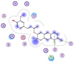
| Iteration 1 | |||||||
|---|---|---|---|---|---|---|---|
| Model | Atom Ligand (ID) | Atom Receptor | Res. Receptor | Chain (Monomer) | Interaction Type | Distance (Å) | E (kcal/mol) |
| 1 | O14 (19) | O | LYS 136 | B | H-donor | 3.22 | −0.6 |
| O10 (10) | CB | ASN 65 | B | H-acceptor | 3.26 | −0.6 | |
| O10 (10) | ND2 | ASN 65 | B | H-acceptor | 3.05 | −1.4 | |
| 6-ring | NZ | LYS 136 | B | pi-cation | 4.74 | −2.2 | |
| 2 | C16 (14) | O | GLN 15 | A | H-donor | 3.45 | −0.5 |
| 3 | O10 (10) | CB | ASN 65 | A | H-acceptor | 3.26 | −0.6 |
| O10 (10) | ND2 | ASN 65 | A | H-acceptor | 3.01 | −1.7 | |
| O15 (21) | 5-ring | HIS 80 | A | H-pi | 4.35 | −1.3 | |
| 6-ring | NZ | LYS 136 | A | pi-cation | 4.90 | −2.0 | |
| 4 | O10 (10) | CB | PRO 62 | A | H-acceptor | 3.06 | −0.5 |
| O10 (10) | N | HIS 63 | A | H-acceptor | 3.07 | −0.6 | |
| 6-ring | ND2 | ASN 65 | A | pi-H | 3.64 | −0.5 | |
| 5 | O10 (10) | CB | PRO 62 | B | H-acceptor | 3.11 | −0.5 |
| O10 (10) | N | HIS 63 | B | H-acceptor | 3.10 | −0.8 | |
| 6-ring | ND2 | ASN 65 | B | pi-H | 3.58 | −0.5 | |
| 6 | O10 (10) | ND2 | ASN 65 | B | H-acceptor | 2.80 | −5.1 |
| O12 (12) | N | HIS 63 | B | H-acceptor | 3.16 | −0.8 | |
| 7 | 6-ring | ND2 | ASN 65 | A | pi-H | 3.59 | −0.8 |
| 6-ring | NZ | LYS 70 | A | pi-cation | 4.04 | −1.4 | |
| 8 | 6-ring | ND2 | ASN 65 | B | pi-H | 3.62 | −0.8 |
| 9 | O10 (10) | NH1 | ARG 115 | B | H-acceptor | 3.05 | −1.8 |
| O10 (10) | NH2 | ARG 115 | B | H-acceptor | 3.10 | −3.7 | |
| 10 | C11 (11) | O | GLN 15 | A | H-donor | 3.34 | −0.8 |
| O12 (12) | O | GLN 15 | A | H-donor | 3.70 | −0.5 | |
| Iteration 2 | |||||||
| Model | Atom Ligand (ID) | Atom Receptor | Res. Receptor | Chain (monomer) | Interaction type | Distance (Å) | E (kcal/mol) |
| 1 | O14 (19) | O | LYS 136 | B | H-donor | 3.17 | −0.6 |
| O10 (10) | ND2 | ASN 65 | B | H-acceptor | 3.02 | −1.5 | |
| 6-ring | NZ | LYS 136 | B | pi-cation | 4.88 | −2.2 | |
| 2 | O10 (10) | CB | ASN 65 | A | H-acceptor | 3.25 | −0.6 |
| O10 (10) | ND2 | ASN 65 | A | H-acceptor | 3.00 | −1.6 | |
| 6-ring | NZ | LYS 136 | A | pi-cation | 4.84 | −2.1 | |
| O14 (19) | 5-ring | HIS 80 | A | H-pi | 4.24 | −1.2 | |
| 3 | O10 (10) | ND2 | ASN 65 | B | H-acceptor | 2.84 | −5.1 |
| O14 (19) | 5-ring | HIS 80 | B | H-pi | 4.39 | −1.4 | |
| 6-ring | NZ | LYS 136 | B | pi-cation | 4.88 | −2.0 | |
| 4 | O10 (10) | CB | ASN 65 | A | H-acceptor | 3.27 | −0.6 |
| O10 (10) | ND2 | ASN 65 | A | H-acceptor | 3.01 | −1.5 | |
| 6-ring | NZ | LYS 136 | A | pi-cation | 4.93 | −2.0 | |
| 5 | O10 (10) | CB | ASN 65 | B | H-acceptor | 3.27 | −0.6 |
| O10 (10) | ND2 | ASN 65 | B | H-acceptor | 3.06 | −1.6 | |
| 6-ring | NZ | LYS 136 | B | pi-cation | 4.82 | −2.2 | |
| 6 | O10 (10) | ND2 | ASN 65 | A | H-acceptor | 2.86 | −4.8 |
| O14 (19) | 5-ring | HIS 80 | A | H-pi | 4.31 | −1.3 | |
| 7 | O10 (10) | ND2 | ASN 65 | B | H-acceptor | 2.93 | −5.2 |
| O14 (19) | 5-ring | HIS 80 | B | H-pi | 4.25 | −1.4 | |
| 8 | O10 (10) | CB | ASN 65 | A | H-acceptor | 3.25 | −0.6 |
| O10 (10) | ND2 | ASN 65 | A | H-acceptor | 3.04 | −1.5 | |
| 9 | O10 (10) | CB | ASN 65 | B | H-acceptor | 3.28 | −0.6 |
| O10 (10) | ND2 | ASN 65 | B | H-acceptor | 3.05 | −1.5 | |
| 10 | O14 (19) | O | LYS 136 | A | H-donor | 3.34 | −0.6 |
| 6-ring | NZ | LYS 136 | A | pi-cation | 4.87 | −2.2 | |
| Iteration 3 | |||||||
| Model | Atom Ligand (ID) | Atom Receptor | Res. Receptor | Chain (monomer) | Interaction type | Distance (Å) | E (kcal/mol) |
| 1 | O10 (10) | ND2 | ASN 65 | B | H-acceptor | 3.09 | −1.5 |
| 6-ring | CA | GLY 141 | B | pi-H | 3.82 | −0.5 | |
| 6-ring | CD | LYS 136 | B | pi-H | 3.80 | −0.6 | |
| 2 | O10 (10) | ND2 | ASN 65 | A | H-acceptor | 3.03 | −1.5 |
| 6-ring | CA | GLY 141 | A | pi-H | 3.77 | −0.6 | |
| 6-ring | CD | LYS 136 | A | pi-H | 3.81 | −0.6 | |
| 3 | O10 (10) | ND2 | ASN 65 | B | H-acceptor | 3.04 | −1.5 |
| 6-ring | CA | GLY 141 | B | pi-H | 3.77 | −0.6 | |
| 6-ring | CD | LYS 136 | B | pi-H | 3.79 | −0.6 | |
| 4 | O10 (10) | ND2 | ASN 65 | A | H-acceptor | 2.97 | −1.5 |
| 6-ring | CA | GLY 141 | A | pi-H | 3.76 | −0.5 | |
| 6-ring | CD | LYS 136 | A | pi-H | 3.78 | −0.5 | |
| 5 | O10 (10) | ND2 | ASN 65 | B | H-acceptor | 2.91 | −1.6 |
| 6-ring | CA | GLY 141 | B | pi-H | 3.73 | −0.6 | |
| 6-ring | CD | LYS 136 | B | pi-H | 3.79 | −0.5 | |
| 6 | O10 (10) | ND2 | ASN 65 | A | H-acceptor | 2.93 | −1.5 |
| 6-ring | CA | GLY 141 | A | pi-H | 3.71 | −0.6 | |
| 6-ring | CD | LYS 136 | A | pi-H | 3.74 | −0.5 | |
| 7 | O10 (10) | ND2 | ASN 65 | B | H-acceptor | 2.92 | −1.5 |
| 6-ring | CA | GLY 141 | B | pi-H | 3.76 | −0.6 | |
| 6-ring | CD | LYS 136 | B | pi-H | 3.75 | −0.6 | |
| 8 | O10 (10) | ND2 | ASN 65 | A | H-acceptor | 2.95 | −1.4 |
| 6-ring | CA | GLY 141 | A | pi-H | 3.78 | −0.6 | |
| 6-ring | CD | LYS 136 | A | pi-H | 3.72 | −0.6 | |
| 9 | O10 (10) | ND2 | ASN 65 | B | H-acceptor | 2.90 | −1.5 |
| 6-ring | CA | GLY 141 | B | pi-H | 3.75 | −0.6 | |
| 6-ring | CD | LYS 136 | B | pi-H | 3.70 | −0.6 | |
| 10 | O10 (10) | ND2 | ASN 65 | A | H-acceptor | 2.91 | −1.5 |
| 6-ring | CA | GLY 141 | A | pi-H | 3.74 | −0.6 | |
| 6-ring | CD | LYS 136 | A | pi-H | 3.69 | −0.6 | |
| Iteration 4 | |||||||
| Model | Atom Ligand (ID) | Atom Receptor | Res. Receptor | Chain (monomer) | Interaction type | Distance (Å) | E (kcal/mol) |
| 1 | O10 (10) | CB | ASN 65 | B | H-acceptor | 3.26 | −0.6 |
| O10 (10) | ND2 | ASN 65 | B | H-acceptor | 3.05 | −1.4 | |
| 6-ring | NZ | LYS 136 | B | pi-cation | 4.73 | −2.3 | |
| 2 | O10 (10) | CB | ASN 65 | A | H-acceptor | 3.27 | −0.6 |
| O10 (10) | ND2 | ASN 65 | A | H-acceptor | 3.03 | −1.6 | |
| 6-ring | NZ | LYS 136 | A | pi-cation | 4.89 | −2.0 | |
| 3 | C17 (18) | O | GLN 15 | A | H-donor | 3.50 | −0.5 |
| 4 | O14 (19) | O | ASN 65 | A | H-donor | 3.18 | −1.0 |
| O10 (10) | CB | PRO 62 | A | H-acceptor | 3.05 | −0.5 | |
| O10 (10) | N | HIS 63 | A | H-acceptor | 3.07 | −0.6 | |
| 6-ring | ND2 | ASN 65 | A | pi-H | 3.64 | −0.5 | |
| 5 | O15 (21) | O | HIS 63 | B | H-donor | 2.85 | −0.7 |
| O10 (10) | CB | PRO 62 | B | H-acceptor | 3.12 | −0.5 | |
| O10 (10) | N | HIS 63 | B | H-acceptor | 3.11 | −0.7 | |
| 6-ring | ND2 | ASN 65 | B | pi-H | 3.58 | −0.5 | |
| 6 | O10 (10) | ND2 | ASN 65 | A | H-acceptor | 2.81 | −5.1 |
| O12 (12) | N | HIS 63 | A | H-acceptor | 3.13 | −0.8 | |
| 7 | O10 (10) | ND2 | ASN 65 | B | H-acceptor | 2.80 | −5.1 |
| O12 (12) | N | HIS 63 | B | H-acceptor | 3.15 | −0.8 | |
| O15 (21) | 5-ring | HIS 80 | B | H-pi | 4.83 | −2.0 | |
| 8 | O12 (12) | O | ASN 53 | B | H-donor | 2.96 | −0.5 |
| 6-ring | NZ | LYS 9 | A | pi-cation | 3.61 | −4.0 | |
| 9 | — | — | — | — | — | — | — |
| 10 | — | — | — | — | — | — | — |
| Iteration 5 | |||||||
| Model | Atom Ligand (ID) | Atom Receptor | Res. Receptor | Chain (monomer) | Interaction type | Distance (Å) | E (kcal/mol) |
| 1 | O10 (10) | CB | ASN 65 | A | H-acceptor | 3.27 | −0.6 |
| O10 (10) | ND2 | ASN 65 | A | H-acceptor | 3.03 | −1.4 | |
| 6-ring | NZ | LYS 136 | A | pi-cation | 4.70 | −2.3 | |
| 2 | O10 (10) | CB | ASN 65 | B | H-acceptor | 3.27 | −0.6 |
| O10 (10) | ND2 | ASN 65 | B | H-acceptor | 3.04 | −1.4 | |
| 6-ring | NZ | LYS 136 | B | pi-cation | 4.85 | −2.1 | |
| 3 | O10 (10) | ND2 | ASN 65 | A | H-acceptor | 2.84 | −5.1 |
| O12 (12) | N | HIS 63 | A | H-acceptor | 3.16 | −0.8 | |
| 4 | O10 (10) | ND2 | ASN 65 | B | H-acceptor | 2.83 | −5.1 |
| O12 (12) | N | HIS 63 | B | H-acceptor | 3.15 | −0.8 | |
| 5 | O14 (19) | O | ASN 65 | B | H-donor | 3.14 | −1.0 |
| O10 (10) | CB | PRO 62 | B | H-acceptor | 3.05 | −0.5 | |
| O10 (10) | N | HIS 63 | B | H-acceptor | 3.04 | −0.6 | |
| 6-ring | ND2 | ASN 65 | B | pi-H | 3.67 | −0.5 | |
| 6 | O14 (19) | O | ASN 65 | A | H-donor | 3.18 | −1.0 |
| O10 (10) | CB | PRO 62 | A | H-acceptor | 3.05 | −0.5 | |
| O10 (10) | N | HIS 63 | A | H-acceptor | 3.06 | −0.6 | |
| 6-ring | ND2 | ASN 65 | A | pi-H | 3.63 | −0.5 | |
| 7 | O12 (12) | O | ASN 53 | A | H-donor | 2.99 | −0.5 |
| 6-ring | NZ | LYS 9 | B | pi-cation | 3.62 | −3.9 | |
| 8 | C17 (18) | O | GLN 15 | B | H-donor | 3.46 | −0.5 |
| 9 | O15 (21) | O | HIS 63 | B | H-donor | 2.86 | −0.7 |
| O10 (10) | CB | PRO 62 | B | H-acceptor | 3.12 | −0.5 | |
| O10 (10) | N | HIS 63 | B | H-acceptor | 3.12 | −0.7 | |
| 6-ring | ND2 | ASN 65 | B | pi-H | 3.59 | −0.5 | |
| 10 | — | — | — | — | — | — | — |
| Iteration 6 | |||||||
| Model | Atom Ligand (ID) | Atom Receptor | Res. Receptor | Chain (monomer) | Interaction type | Distance (Å) | E (kcal/mol) |
| 1 | O12 (12) | O | ASN 53 | A | H-donor | 3.04 | −0.5 |
| O10 (10) | ND2 | ASN 65 | A | H-acceptor | 2.81 | −5.3 | |
| 6-ring | ND2 | ASN 65 | A | pi-H | 3.66 | −0.5 | |
| 2 | O10 (10) | ND2 | ASN 65 | B | H-acceptor | 2.82 | −5.2 |
| O12 (12) | O | ASN 53 | B | H-donor | 3.04 | −0.5 | |
| 6-ring | ND2 | ASN 65 | B | pi-H | 3.63 | −0.5 | |
| 3 | O10 (10) | CB | ASN 65 | A | H-acceptor | 3.26 | −0.6 |
| O10 (10) | ND2 | ASN 65 | A | H-acceptor | 3.03 | −1.4 | |
| 6-ring | NZ | LYS 136 | A | pi-cation | 4.65 | −2.2 | |
| 4 | O10 (10) | CB | ASN 65 | B | H-acceptor | 3.29 | −0.6 |
| O10 (10) | ND2 | ASN 65 | B | H-acceptor | 3.01 | −1.4 | |
| 6-ring | NZ | LYS 136 | B | pi-cation | 4.72 | −2.1 | |
| 5 | O10 (10) | N | HIS 63 | B | H-acceptor | 3.09 | −0.6 |
| 6-ring | ND2 | ASN 65 | B | pi-H | 3.64 | −0.5 | |
| O10 (10) | CB | PRO 62 | B | H-acceptor | 3.10 | −0.5 | |
| 6 | O10 (10) | N | HIS 63 | A | H-acceptor | 3.07 | −0.6 |
| 6-ring | ND2 | ASN 65 | A | pi-H | 3.58 | −0.5 | |
| O10 (10) | CB | PRO 62 | A | H-acceptor | 3.11 | −0.5 | |
| 7 | O12 (12) | O | ASN 53 | B | H-donor | 2.97 | −0.5 |
| 6-ring | NZ | LYS 9 | A | pi-cation | 3.70 | −3.9 | |
| 8 | O10 (10) | CB | ASN 65 | B | H-acceptor | 3.22 | −0.6 |
| O10 (10) | ND2 | ASN 65 | B | H-acceptor | 2.95 | −1.5 | |
| 6-ring | NZ | LYS 136 | B | pi-cation | 4.40 | −2.2 | |
| 9 | C17 (18) | O | GLN 15 | B | H-donor | 3.30 | −0.5 |
| 10 | O10 (10) | ND2 | ASN 65 | A | H-acceptor | 2.83 | −5.3 |
| O12 (12) | O | ASN 53 | A | H-donor | 3.01 | −0.5 | |
| 6-ring | ND2 | ASN 65 | A | pi-H | 3.66 | −0.5 | |
| Iteration 7 | |||||||
| Model | Atom Ligand (ID) | Atom Receptor | Res. Receptor | Chain (monomer) | Interaction type | Distance (Å) | E (kcal/mol) |
| 1 | O10 | CB | ASN 65 | B | H-acceptor | 3.26 | −0.6 |
| O10 | ND2 | ASN 65 | B | H-acceptor | 3.04 | −1.4 | |
| 6-ring | NZ | LYS 136 | B | pi-cation | 4.72 | −2.3 | |
| 2 | C16 | O | GLN 15 | A | H-donor | 3.45 | −0.5 |
| O14 | O | THR 54 | B | H-donor | 3.04 | −1.9 | |
| 3 | O10 | CB | ASN 65 | A | H-acceptor | 3.27 | −0.6 |
| O10 | ND2 | ASN 65 | A | H-acceptor | 3.04 | −1.7 | |
| 6-ring | NZ | LYS 136 | A | pi-cation | 4.89 | −2.1 | |
| 4 | O10 | CB | PRO 62 | B | H-acceptor | 3.11 | −0.5 |
| O10 | N | HIS 63 | B | H-acceptor | 3.09 | −0.8 | |
| 6-ring | ND2 | ASN 65 | B | pi-H | 3.59 | −0.5 | |
| 5 | O10 | CB | PRO 62 | A | H-acceptor | 3.06 | −0.5 |
| O10 | N | HIS 63 | A | H-acceptor | 3.07 | −0.6 | |
| 6-ring | ND2 | ASN 65 | A | pi-H | 3.64 | −0.5 | |
| 6 | O10 | ND2 | ASN 65 | A | H-acceptor | 2.80 | −5.0 |
| O12 | N | HIS 63 | A | H-acceptor | 3.17 | −0.8 | |
| 7 | 6-ring | NZ | LYS 9 | A | pi-cation | 3.63 | −1.2 |
| 8 | O14 | O | THR 135 | A | H-donor | 3.15 | −0.9 |
| 9 | O10 | NH1 | ARG 115 | B | H-acceptor | 3.05 | −1.8 |
| O10 | NH2 | ARG 115 | B | H-acceptor | 3.10 | −3.7 | |
| 10 | O12 | NZ | LYS 122 | A | H-acceptor | 3.22 | −1.2 |
| Iteration 8 | |||||||
| Model | Atom Ligand (ID) | Atom Receptor | Res. Receptor | Chain (monomer) | Interaction type | Distance (Å) | E (kcal/mol) |
| 1 | O12 | NZ | LYS 122 | A | H-acceptor | 3.07 | −1.7 |
| O12 | CD | LYS 122 | A | H-acceptor | 3.59 | −0.4 | |
| 2 | O10 | CB | PRO 62 | A | H-acceptor | 3.06 | −0.5 |
| O10 | N | HIS 63 | A | H-acceptor | 3.09 | −0.6 | |
| 6-ring | ND2 | ASN 65 | A | pi-H | 3.64 | −0.6 | |
| 3 | O14 | N | HIS 63 | B | H-acceptor | 3.15 | −0.9 |
| O14 | CB | PRO 62 | B | H-acceptor | 3.27 | −0.7 | |
| 6-ring | ND2 | ASN 65 | B | pi-H | 3.59 | −0.4 | |
| 4 | O10 | NH1 | ARG 115 | A | H-acceptor | 3.06 | −1.4 |
| O10 | NH2 | ARG 115 | A | H-acceptor | 3.14 | −2.8 | |
| 5 | 6-ring | NZ | LYS 9 | A | pi-cation | 3.92 | −1.1 |
| 6 | O12 | CD | LYS 122 | A | H-acceptor | 3.25 | −0.6 |
| 7 | O10 | O | THR 54 | A | H-donor | 3.09 | −0.9 |
| 8 | O12 | NE | ARG 115 | A | H-acceptor | 3.02 | −1.6 |
| 9 | O12 | CD | LYS 122 | B | H-acceptor | 3.41 | −0.5 |
| 10 | O12 | NZ | LYS 122 | B | H-acceptor | 3.28 | −1.1 |
| Iteration 9 | |||||||
| Model | Atom Ligand (ID) | Atom Receptor | Res. Receptor | Chain (monomer) | Interaction type | Distance (Å) | E (kcal/mol) |
| 1 | O12 | NZ | LYS 122 | A | H-acceptor | 3.09 | −1.5 |
| O12 | CD | LYS 122 | A | H-acceptor | 3.63 | −0.5 | |
| 2 | O10 | CB | PRO 62 | A | H-acceptor | 3.08 | −0.5 |
| O10 | N | HIS 63 | A | H-acceptor | 3.10 | −0.6 | |
| 6-ring | ND2 | ASN 65 | A | pi-H | 3.60 | −0.5 | |
| 3 | O14 | N | HIS 63 | B | H-acceptor | 3.16 | −1.0 |
| O14 | CB | PRO 62 | B | H-acceptor | 3.25 | −0.6 | |
| 6-ring | ND2 | ASN 65 | B | pi-H | 3.62 | −0.5 | |
| 4 | O10 | NH1 | ARG 115 | A | H-acceptor | 3.09 | −1.3 |
| O10 | NH2 | ARG 115 | A | H-acceptor | 3.15 | −2.9 | |
| 5 | 6-ring | NZ | LYS 9 | A | pi-cation | 3.94 | −1.2 |
| 6 | O12 | CD | LYS 122 | A | H-acceptor | 3.27 | −0.7 |
| 7 | O10 | O | THR 54 | A | H-donor | 3.06 | −1.0 |
| 8 | O12 | NE | ARG 115 | A | H-acceptor | 3.05 | −1.7 |
| 9 | O12 | CD | LYS 122 | B | H-acceptor | 3.43 | −0.6 |
| 10 | O12 | NZ | LYS 122 | B | H-acceptor | 3.31 | −1.3 |
| Iteration 10 | |||||||
| Model | Atom Ligand (ID) | Atom Receptor | Res. Receptor | Chain (monomer) | Interaction type | Distance (Å) | E (kcal/mol) |
| 1 | O10 (10) | CB | ASN 65 | B | H-acceptor | 3.26 | −0.6 |
| O10 (10) | ND2 | ASN 65 | B | H-acceptor | 3.04 | −1.4 | |
| 6-ring | NZ | LYS 136 | B | pi-cation | 4.73 | −2.3 | |
| 2 | C16 (14) | O | GLN 15 | A | H-donor | 3.45 | −0.5 |
| 3 | O10 (10) | CB | ASN 65 | A | H-acceptor | 3.26 | −0.6 |
| O10 (10) | ND2 | ASN 65 | A | H-acceptor | 3.04 | −1.6 | |
| 6-ring | NZ | LYS 136 | A | pi-cation | 4.88 | −2.1 | |
| 4 | O10 (10) | CB | PRO 62 | A | H-acceptor | 3.04 | −0.5 |
| O10 (10) | N | HIS 63 | A | H-acceptor | 3.08 | −0.6 | |
| 6-ring | ND2 | ASN 65 | A | pi-H | 3.65 | −0.5 | |
| 5 | O10 (10) | CB | PRO 62 | B | H-acceptor | 3.08 | −0.5 |
| O10 (10) | N | HIS 63 | B | H-acceptor | 3.07 | −1.0 | |
| 6-ring | ND2 | ASN 65 | B | pi-H | 3.61 | −0.5 | |
| 6 | O10 (10) | ND2 | ASN 65 | A | H-acceptor | 2.80 | −5.1 |
| O12 (12) | N | HIS 63 | A | H-acceptor | 3.16 | −0.8 | |
| 7 | O10 (10) | ND2 | ASN 65 | B | H-acceptor | 2.80 | −5.1 |
| O12 (12) | N | HIS 63 | B | H-acceptor | 3.15 | −0.8 | |
| 8 | 6-ring | ND2 | ASN 65 | B | pi-H | 3.62 | −0.8 |
| 9 | C11 (11) | O | GLN 15 | A | H-donor | 3.35 | −0.8 |
| O12 (12) | O | GLN 15 | A | H-donor | 3.68 | −0.5 | |
| 10 | O14 (19) | O | LEU 42 | A | H-donor | 2.75 | −3.9 |
| O12 (12) | NZ | LYS 122 | A | H-acceptor | 3.23 | −1.2 | |
| 6-ring | CG2 | THR 39 | A | pi-H | 3.93 | −0.5 | |
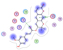
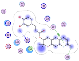
| Iteration 1 | |||||||
|---|---|---|---|---|---|---|---|
| Model | Atom Ligand (ID) | Atom Receptor | Res. Receptor | Chain (Monomer) | Interaction Type | Distance (Å) | E (kcal/mol) |
| 1 | O27 (20) | NZ | LYS 122 | A | H-acceptor | 3.17 | −1.5 |
| 6-ring | CA | ASP 125 | A | pi-H | 3.64 | −0.6 | |
| 2 | O26 (31) | O | GLU 40 | B | H-donor | 2.89 | −1.4 |
| O27 (20) | NZ | LYS 122 | B | H-acceptor | 3.19 | −1.1 | |
| 3 | O27 (20) | CA | PRO 66 | A | H-acceptor | 3.57 | −0.5 |
| O24 (29) | NH2 | ARG 115 | A | H-acceptor | 3.10 | −1.4 | |
| 4 | — | — | — | — | — | — | — |
| 5 | C25 (30) | O | ASP 109 | B | H-donor | 3.77 | −0.5 |
| O27 (20) | CA | PRO 66 | B | H-acceptor | 3.64 | −0.5 | |
| 6 | O27 (20) | CA | PRO 62 | A | H-acceptor | 3.35 | −1.1 |
| 6-ring | CG | LYS 136 | A | pi-H | 3.64 | −0.5 | |
| 7 | C7 (7) | OG1 | THR 137 | B | H-donor | 3.52 | −0.6 |
| 6-ring | CA | GLY 141 | B | pi-H | 3.78 | −0.5 | |
| 8 | O6 (6) | NE1 | TRP 32 | B | H-acceptor | 3.07 | −1.8 |
| 9 | — | — | — | — | — | — | — |
| 10 | O24 (29) | ND2 | ASN 65 | A | H-acceptor | 3.02 | −1.5 |
| Iteration 2 | |||||||
| Model | Atom Ligand (ID) | Atom Receptor | Res. Receptor | Chain (monomer) | Interaction type | Distance (Å) | E (kcal/mol) |
| 1 | O26 (31) | NH1 | ARG 141 | A | H-donor | 3.10 | −1.3 |
| 6-ring | CG | ASP 145 | A | pi-H | 3.50 | −0.7 | |
| 2 | O27 (20) | OD1 | ASP 108 | B | H-acceptor | 3.00 | −1.5 |
| C7 (7) | OG1 | THR 132 | A | H-donor | 3.45 | −0.6 | |
| 3 | O6 (6) | NE | ARG 115 | A | H-acceptor | 3.20 | −1.2 |
| 6-ring | CA | PRO 66 | B | pi-H | 3.55 | −0.5 | |
| 4 | — | — | — | — | — | — | — |
| 5 | C25 (30) | OE1 | GLU 124 | A | H-donor | 3.60 | −0.7 |
| O27 (20) | CA | PRO 62 | B | H-acceptor | 3.33 | −1.0 | |
| 6 | O26 (31) | OG | SER 139 | A | H-donor | 3.15 | −1.3 |
| 6-ring | CB | LYS 122 | B | pi-H | 3.70 | −0.5 | |
| 7 | C7 (7) | OG1 | THR 137 | B | H-donor | 3.40 | −0.8 |
| 6-ring | CA | GLY 141 | A | pi-H | 3.77 | −0.6 | |
| 8 | O24 (29) | ND2 | ASN 65 | B | H-acceptor | 3.09 | −1.6 |
| 9 | — | — | — | — | — | — | — |
| 10 | O27 (20) | NZ | LYS 122 | A | H-acceptor | 3.11 | −1.5 |
| Iteration 3 | |||||||
| Model | Atom Ligand (ID) | Atom Receptor | Res. Receptor | Chain (monomer) | Interaction type | Distance (Å) | E (kcal/mol) |
| 1 | O6 (6) | ND1 | HIS 46 | A | H-acceptor | 3.25 | −1.4 |
| 6-ring | CG | ASP 125 | B | pi-H | 3.60 | −0.5 | |
| 2 | O27 (20) | NZ | LYS 136 | B | H-acceptor | 3.12 | −1.3 |
| C7 (7) | OG1 | THR 137 | A | H-donor | 3.49 | −0.6 | |
| 3 | O26 (31) | NE | ARG 115 | A | H-acceptor | 3.18 | −1.2 |
| 6-ring | CA | PRO 66 | B | pi-H | 3.50 | −0.5 | |
| 4 | — | — | — | — | — | — | — |
| 5 | C25 (30) | OE2 | GLU 40 | B | H-donor | 3.59 | −0.6 |
| O24 (29) | CA | PRO 62 | A | H-acceptor | 3.32 | −0.9 | |
| 6 | O27 (20) | CA | PRO 66 | A | H-acceptor | 3.40 | −1.1 |
| 6-ring | CG | LYS 136 | A | pi-H | 3.66 | −0.4 | |
| 7 | C7 (7) | OG1 | THR 137 | A | H-donor | 3.41 | −0.7 |
| 6-ring | CA | GLY 141 | B | pi-H | 3.76 | −0.6 | |
| 8 | O26 (31) | NE1 | TRP 32 | B | H-acceptor | 3.06 | −1.9 |
| 9 | — | — | — | — | — | — | — |
| 10 | O27 (20) | ND2 | ASN 65 | A | H-acceptor | 3.01 | −1.4 |
| Iteration 4 | |||||||
| Model | Atom Ligand (ID) | Atom Receptor | Res. Receptor | Chain (monomer) | Interaction type | Distance (Å) | E (kcal/mol) |
| 1 | O4 (4) | CA | SER 68 | A | H-acceptor | 3.74 | −0.5 |
| 2 | O6 (20) | OE2 | GLU 132 | B | H-donor | 3.09 | −1.9 |
| 3 | O6 (20) | O | ARG 69 | B | H-donor | 3.18 | −1.0 |
| 4 | — | — | — | — | — | — | — |
| 5 | — | — | — | — | — | — | — |
| 6 | — | — | — | — | — | — | — |
| 7 | — | — | — | — | — | — | — |
| 8 | O6 (20) | OG1 | THR 39 | B | H-acceptor | 2.73 | −0.6 |
| 9 | — | — | — | — | — | — | — |
| 10 | — | — | — | — | — | — | — |
| Iteration 5 | |||||||
| Model | Atom Ligand (ID) | Atom Receptor | Res. Receptor | Chain (monomer) | Interaction type | Distance (Å) | E (kcal/mol) |
| 1 | O4 (4) | CA | SER 68 | A | H-acceptor | 3.66 | −0.5 |
| 2 | O7 (22) | OE2 | GLU 132 | B | H-donor | 2.70 | −4.5 |
| 3 | O7 (22) | O | ARG 69 | A | H-donor | 3.01 | −1.4 |
| 4 | — | — | — | — | — | — | — |
| 5 | O6 (20) | O | THR 135 | B | H-donor | 2.93 | −1.9 |
| 6 | 6-ring | NZ | LYS 9 | A | pi-cation | 3.83 | −1.1 |
| 7 | O6 (20) | O | GLU 121 | B | H-donor | 3.03 | −1.6 |
| O5 (24) | O | ALA 123 | B | H-donor | 3.17 | −0.9 | |
| 8 | — | — | — | — | — | — | — |
| 9 | O6 (20) | 5-ring | HIS 80 | B | H-pi | 4.12 | −3.4 |
| 10 | — | — | — | — | — | — | — |
| Iteration 6 | |||||||
| Model | Atom Ligand (ID) | Atom Receptor | Res. Receptor | Chain (monomer) | Interaction type | Distance (Å) | E (kcal/mol) |
| 1 | — | — | — | — | — | — | — |
| 2 | O4 (4) | CA | SER 68 | A | H-acceptor | 3.63 | −0.5 |
| 3 | O7 (22) | OE2 | GLU 132 | B | H-donor | 2.70 | −2.9 |
| 4 | O6 (20) | NE2 | HIS 80 | B | H-acceptor | 3.04 | −0.6 |
| 5 | — | — | — | — | — | — | — |
| 6 | O7 (22) | O | ARG 69 | A | H-donor | 2.94 | −1.8 |
| 7 | — | — | — | — | — | — | — |
| 8 | 6-ring | NZ | LYS 9 | A | pi-cation | 3.83 | −1.1 |
| 9 | O6 (20) | O | LEU 84 | B | H-donor | 3.02 | −1.9 |
| 10 | — | — | — | — | — | — | — |
| Iteration 7 | |||||||
| Model | Atom Ligand (ID) | Atom Receptor | Res. Receptor | Chain (monomer) | Interaction type | Distance (Å) | E (kcal/mol) |
| 1 | O4 (4) | CA | SER 68 | A | H-acceptor | 3.67 | −0.5 |
| 2 | — | — | — | — | — | — | — |
| 3 | O6 (20) | O | THR 135 | B | H-donor | 2.70 | −1.4 |
| 4 | O6 (20) | O | THR 135 | A | H-donor | 2.75 | −0.7 |
| 5 | — | — | — | — | — | — | — |
| 6 | O6 (20) | O | LEU 84 | A | H-donor | 3.06 | −0.8 |
| 7 | O5 (24) | O | SER 34 | A | H-donor | 2.89 | −0.8 |
| 6-ring | NZ | LYS 9 | A | pi-cation | 3.83 | −1.1 | |
| 8 | — | — | — | — | — | — | — |
| 9 | O6 (20) | O | LEU 84 | B | H-donor | 3.02 | −2.1 |
| 10 | O5 (24) | O | ASN 53 | B | H-donor | 2.99 | −0.9 |
| 6-ring | NZ | LYS 9 | A | pi-cation | 3.79 | −0.7 | |
| Iteration 8 | |||||||
| Model | Atom Ligand (ID) | Atom Receptor | Res. Receptor | Chain (monomer) | Interaction type | Distance (Å) | E (kcal/mol) |
| 1 | O4 (4) | CA | SER 68 | A | H-acceptor | 3.64 | −0.5 |
| 2 | O6 (20) | OE2 | GLU 132 | B | H-donor | 3.10 | −3.9 |
| 3 | O6 (20) | O | ARG 69 | B | H-donor | 3.21 | −1.2 |
| O7 (22) | O | ARG 69 | B | H-donor | 2.98 | −1.5 | |
| 4 | O6 (20) | O | ARG 69 | A | H-donor | 3.25 | −1.3 |
| 5 | O5 (24) | O | ALA 123 | A | H-donor | 3.16 | −0.8 |
| 6 | O5 (24) | O | PRO 74 | A | H-donor | 3.20 | −1.2 |
| 7 | O7 (22) | O | ASN 86 | B | H-donor | 2.75 | −3.1 |
| 8 | O5 (24) | O | SER 34 | A | H-donor | 2.89 | −1.4 |
| 6-ring | NZ | LYS 9 | A | pi-cation | 3.83 | −1.1 | |
| 9 | O6 (20) | O | GLN 15 | A | H-donor | 2.70 | −1.1 |
| 6-ring | NZ | LYS 9 | A | pi-cation | 3.80 | −0.7 | |
| 10 | — | — | — | — | — | — | — |
| Iteration 9 | |||||||
| Model | Atom Ligand (ID) | Atom Receptor | Res. Receptor | Chain (monomer) | Interaction type | Distance (Å) | E (kcal/mol) |
| 1 | O6 (20) | OE2 | GLU 132 | A | H-donor | 3.16 | −1.3 |
| O4 (4) | CA | SER 68 | A | H-acceptor | 3.64 | −0.5 | |
| 2 | — | — | — | — | — | — | — |
| 3 | — | — | — | — | — | — | — |
| 4 | O6 (20) | O | THR 135 | A | H-donor | 2.74 | −0.9 |
| 5 | O6 (20) | O | GLU 121 | A | H-donor | 3.00 | −2.0 |
| O5 (24) | O | ALA 123 | A | H-donor | 3.15 | −1.4 | |
| 6 | O6 (20) | O | LEU 84 | A | H-donor | 3.05 | −0.9 |
| O7 (22) | O | ASN 86 | A | H-donor | 2.70 | −2.4 | |
| O5 (24) | O | PRO 74 | A | H-donor | 3.18 | −1.0 | |
| 7 | O6 (20) | O | LEU 84 | B | H-donor | 3.02 | −1.8 |
| 8 | O5 (24) | O | GLN 15 | A | H-donor | 2.75 | −1.4 |
| 6-ring | NZ | LYS 9 | A | pi-cation | 3.83 | −1.1 | |
| 9 | O7 22 | O | GLU 40 | B | H-donor | 2.86 | −1.5 |
| 10 | O6 20 | O | SER 34 | A | H-donor | 2.97 | −1.4 |
| O5 24 | O | ASN 53 | B | H-donor | 2.99 | −0.5 | |
| 6-ring | NZ | LYS 9 | A | pi-cation | 3.79 | −0.7 | |
| Iteration 10 | |||||||
| Model | Atom Ligand (ID) | Atom Receptor | Res. Receptor | Chain (monomer) | Interaction type | Distance (Å) | E (kcal/mol) |
| 1 | O4 (4) | CA | SER 68 | A | H-acceptor | 3.63 | −0.5 |
| 2 | — | — | — | — | — | — | — |
| 3 | — | — | — | — | — | — | — |
| 4 | O6 (20) | O | THR 135 | A | H-donor | 2.75 | −3.0 |
| O6 (20) | CA | LYS 70 | A | H-acceptor | 3.33 | −0.6 | |
| 5 | — | — | — | — | — | — | — |
| 6 | O6 (20) | O | ASN 86 | A | H-donor | 2.95 | −2.2 |
| O5 (24) | O | PRO 74 | A | H-donor | 3.19 | −1.3 | |
| 7 | 6-ring | NZ | LYS 9 | A | pi-cation | 3.82 | −1.1 |
| 8 | O5 (24) | O | ALA 123 | B | H-donor | 3.13 | −1.1 |
| 9 | — | — | — | — | — | — | — |
| 10 | 6-ring | NZ | LYS 9 | A | pi-cation | 3.79 | −0.7 |
| No. | Ligand Name | Molecular Mass (g/mol) | LogP | H-Bond Donors | H-Bond Acceptors | Lipinski Rule of Five Compliance |
|---|---|---|---|---|---|---|
| 1 | 1-(2,5-dideoxy-5-pyrrolidin-1-yl-β-L-erythro-pentofuranosyl)uracil | 260.00 | 1.5 | 2 | 5 | Yes |
| 2 | 2′,3′-Dideoxythymidine-5′-Monophosphate | 306.21 | −1.5 | 3 | 7 | Yes |
| 3 | 2′,5′-Dideoxyuridine | 228.00 | −1.0 | 2 | 5 | Yes |
| 4 | 2′-Deoxy-5-(hydroxymethyl)uridine 5′-(dihydrogen phosphate) | 338.21 | −2.0 | 3 | 8 | Yes |
| 5 | 2′-Deoxyuridine | 228.20 | −1.0 | 2 | 5 | Yes |
| 6 | 5′-Deoxy-5′-piperidin-1-ylthymidine | 270.00 | 1.0 | 2 | 5 | Yes |
| 7 | 5-Methyl-2′-fluoroauracil F-18 | 150.00 | 0.5 | 1 | 4 | Yes |
| 8 | Alovudine F-18 | 250.00 | 1.0 | 2 | 5 | Yes |
| 9 | Alovudine | 250.00 | 1.0 | 2 | 5 | Yes |
| 10 | Brivudine Monophosphate | 413.11 | 0.5 | 4 | 8 | Yes |
| 11 | Brivudine | 333.13 | 1.0 | 3 | 6 | Yes |
| 12 | Broxuridine | 306.00 | 0.5 | 2 | 7 | Yes |
| 13 | Clevudine | 272.00 | 1.5 | 2 | 5 | Yes |
| 14 | Ebselen | 274.98 | 3.13 | 0 | 0 | Yes |
| 15 | Edoxudine | 306.00 | 0.5 | 2 | 7 | Yes |
| 16 | Epigallocatechin Gallate | 458.00 | 1.2 | 8 | 11 | No |
| 17 | Ethaselen | 300.00 | 2.0 | 1 | 4 | Yes |
| 18 | Ethylarabinosyluracil | 260.00 | 1.0 | 2 | 5 | Yes |
| 19 | Floxuridine | 264.00 | −1.0 | 2 | 6 | Yes |
| 20 | Idoxuridine | 354.00 | 0.5 | 2 | 7 | Yes |
| 21 | Netivudine | 272.00 | 1.5 | 2 | 5 | Yes |
| 22 | PRG_A01 | 300.00 | 1.0 | 2 | 6 | Yes |
| 23 | Rotenone | 394.00 | 4.0 | 0 | 5 | Yes |
| 24 | S_XL6 | 320.00 | 2.0 | 2 | 6 | Yes |
| 25 | Sorivudine | 316.00 | 1.0 | 2 | 6 | Yes |
| 26 | Telbivudine | 258.00 | 1.5 | 2 | 5 | Yes |
| 27 | Thymidine Monophosphate | 322.00 | −1.5 | 3 | 8 | Yes |
| 28 | Thymidine 3′,5′-Diphosphate | 402.00 | −2.5 | 4 | 10 | Yes |
| 29 | Thymidine 5′-Diphosphate | 402.00 | −2.5 | 4 | 10 | Yes |
| 30 | Thymidine 5′-(dithio)phosphate | 370.00 | −2.0 | 3 | 9 | Yes |
| 31 | Thymidine 5′-Thiophosphate | 354.00 | −2.0 | 3 | 8 | Yes |
| 32 | TMP (Thymidine Monophosphate) | 322.00 | −1.5 | 3 | 8 | Yes |
| 33 | Trifluridine | 296.00 | 0.5 | 2 | 7 | Yes |
| 34 | Uridine | 244.00 | −2.0 | 3 | 6 | Yes |
| 35 | Zidovudine | 267.00 | 1.0 | 2 | 6 | Yes |
| 36 | Baicalein | 270.24 | 2.5 | 3 | 5 | Yes |
| 37 | Lovastatin | 404.54 | 4.57 | 1 | 5 | Yes |
| 38 | Quercetin | 302.24 | 1.5 | 5 | 7 | Yes |
| 39 | Simvastatin | 418.57 | 4.68 | 1 | 5 | Yes |
| Ligand Number | Ligand Name | Structural Formula |
|---|---|---|
| 22 | PRG-A01 | 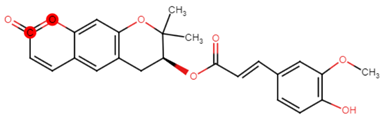 |
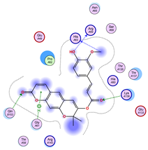
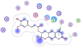
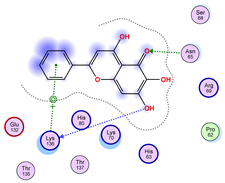
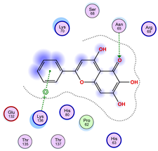
| 36 | Baicalein | 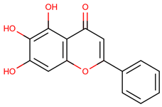 |
| 38 | Quercetin | 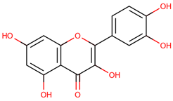 |
| Ligand Number | Ligand Name | Structural Formula |
|---|---|---|
| 34 | Uridine | 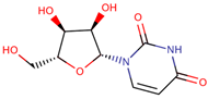 |
| 37 | Lovastatin | 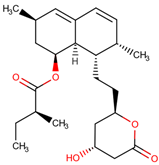 |
| 24 | S-XL6 | 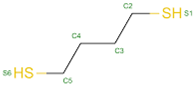 |
Disclaimer/Publisher’s Note: The statements, opinions and data contained in all publications are solely those of the individual author(s) and contributor(s) and not of MDPI and/or the editor(s). MDPI and/or the editor(s) disclaim responsibility for any injury to people or property resulting from any ideas, methods, instructions or products referred to in the content. |
© 2025 by the authors. Licensee MDPI, Basel, Switzerland. This article is an open access article distributed under the terms and conditions of the Creative Commons Attribution (CC BY) license (https://creativecommons.org/licenses/by/4.0/).
Share and Cite
Carnaroli, M.; Deriu, M.A.; Tuszynski, J.A. Computational Search for Inhibitors of SOD1 Mutant Infectivity as Potential Therapeutics for ALS Disease. Int. J. Mol. Sci. 2025, 26, 4660. https://doi.org/10.3390/ijms26104660
Carnaroli M, Deriu MA, Tuszynski JA. Computational Search for Inhibitors of SOD1 Mutant Infectivity as Potential Therapeutics for ALS Disease. International Journal of Molecular Sciences. 2025; 26(10):4660. https://doi.org/10.3390/ijms26104660
Chicago/Turabian StyleCarnaroli, Marco, Marco Agostino Deriu, and Jack Adam Tuszynski. 2025. "Computational Search for Inhibitors of SOD1 Mutant Infectivity as Potential Therapeutics for ALS Disease" International Journal of Molecular Sciences 26, no. 10: 4660. https://doi.org/10.3390/ijms26104660
APA StyleCarnaroli, M., Deriu, M. A., & Tuszynski, J. A. (2025). Computational Search for Inhibitors of SOD1 Mutant Infectivity as Potential Therapeutics for ALS Disease. International Journal of Molecular Sciences, 26(10), 4660. https://doi.org/10.3390/ijms26104660