Deciphering RNA-Recognition Patterns of Intrinsically Disordered Proteins


Abstract
: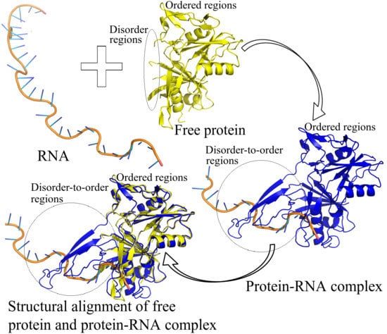
1. Introduction
2. Results and Discussion
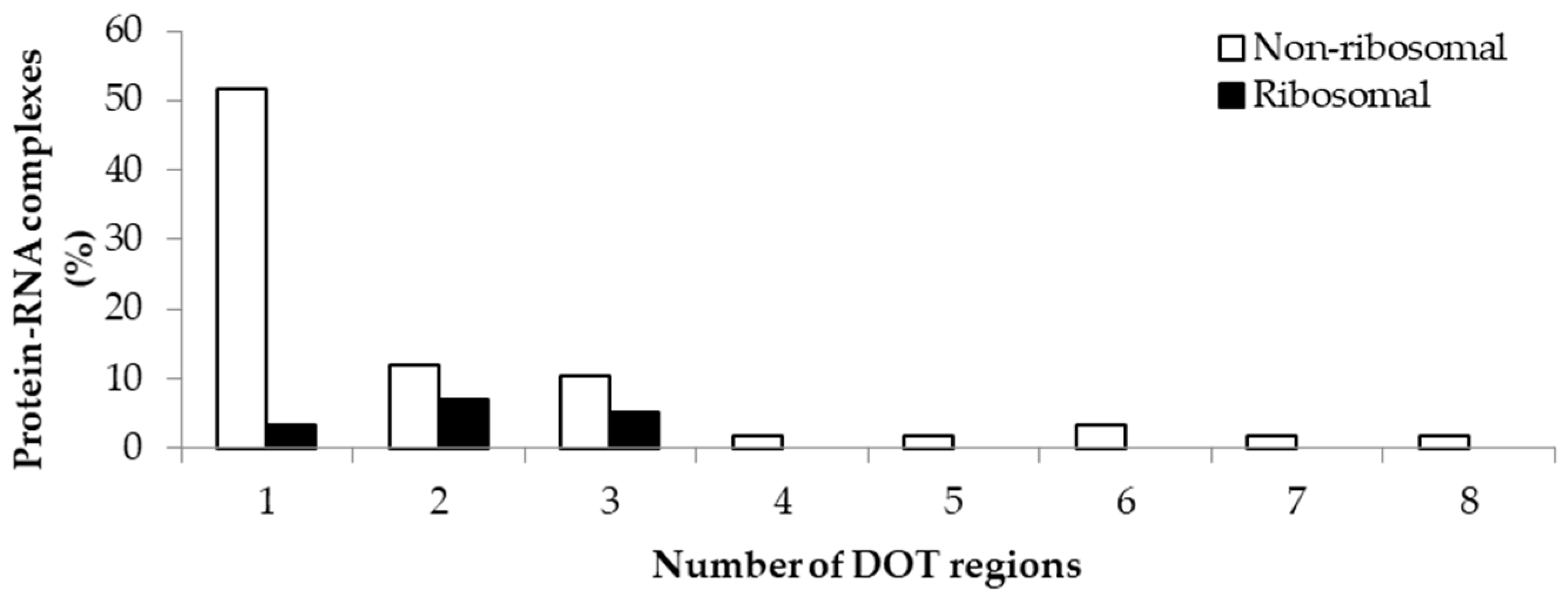
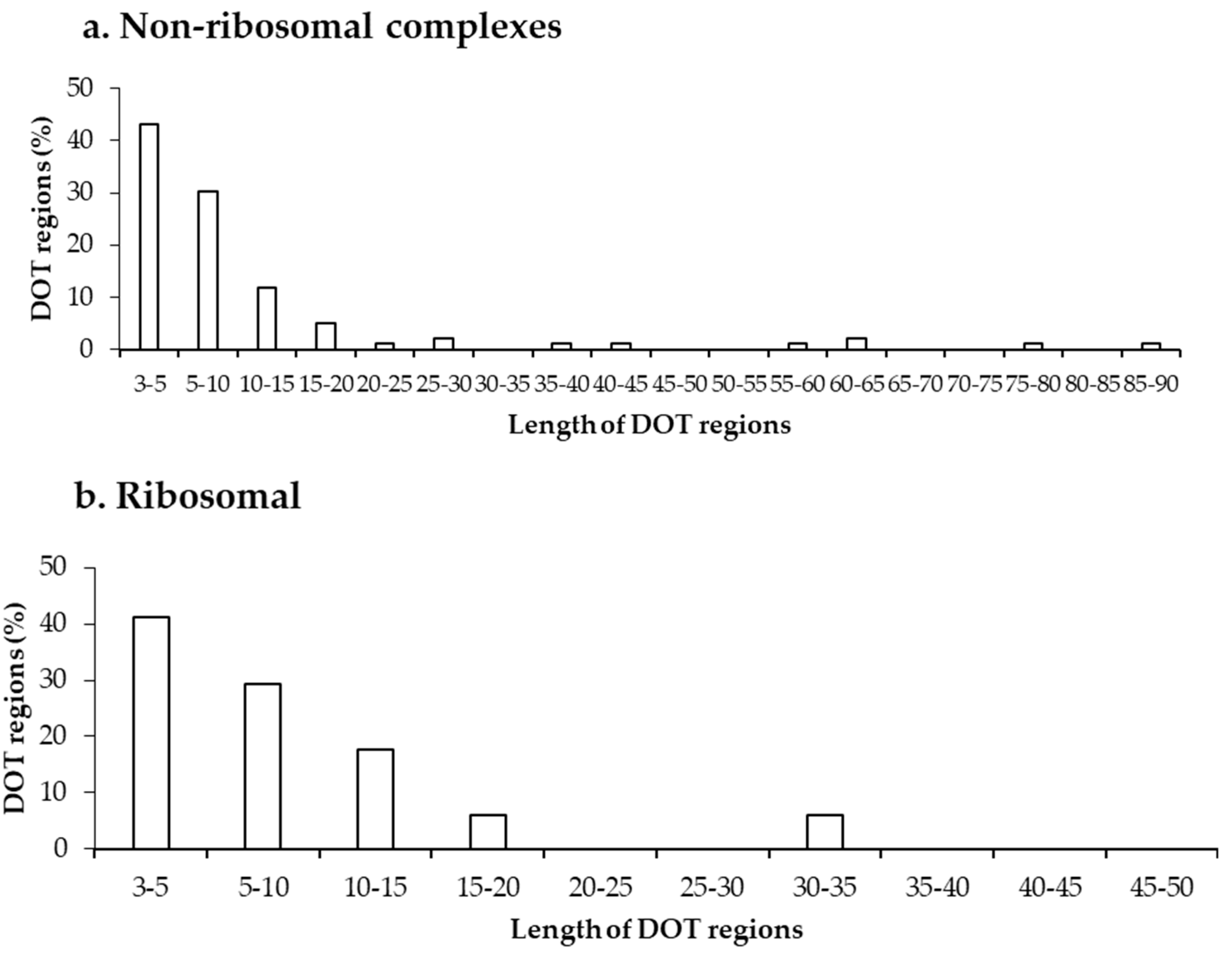
2.1. Number of DOT Regions in Protein–RNA Complexes and Length of DOT Regions
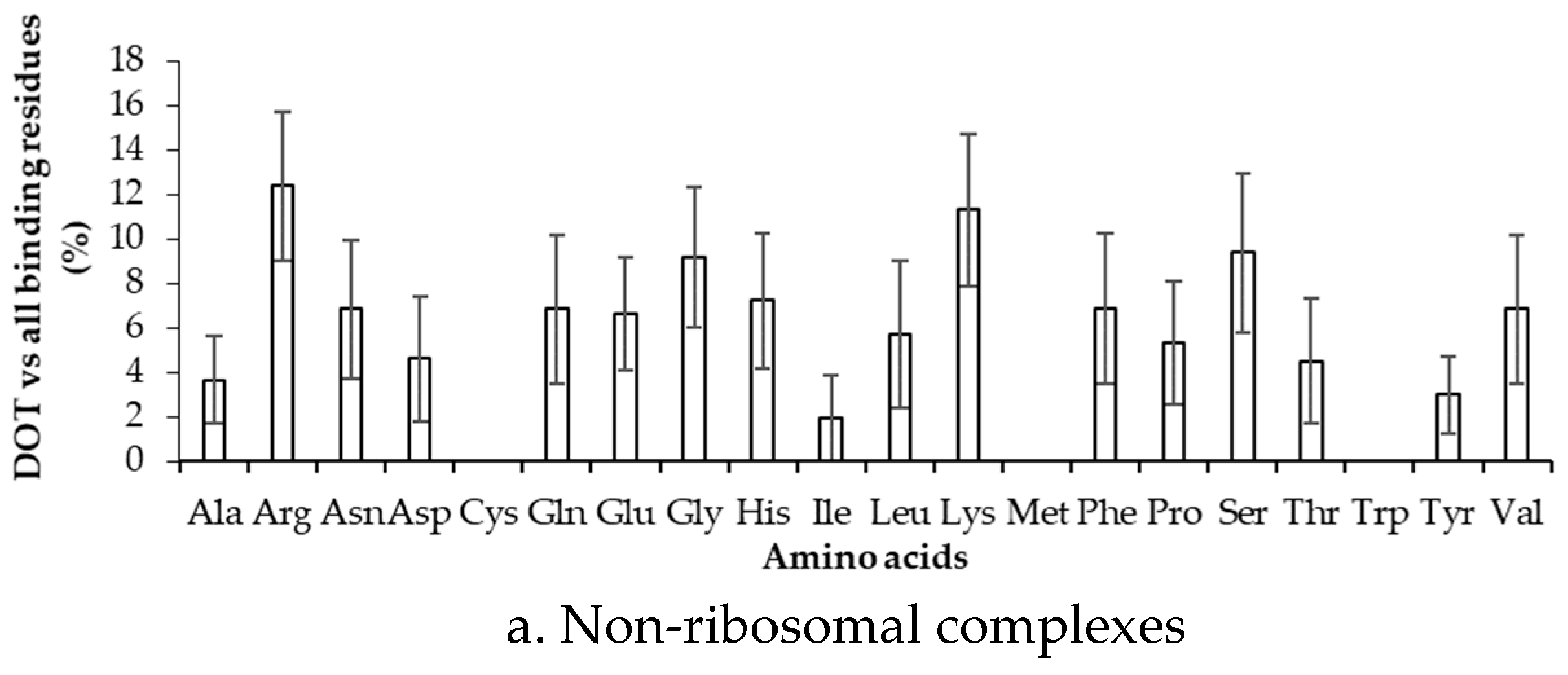
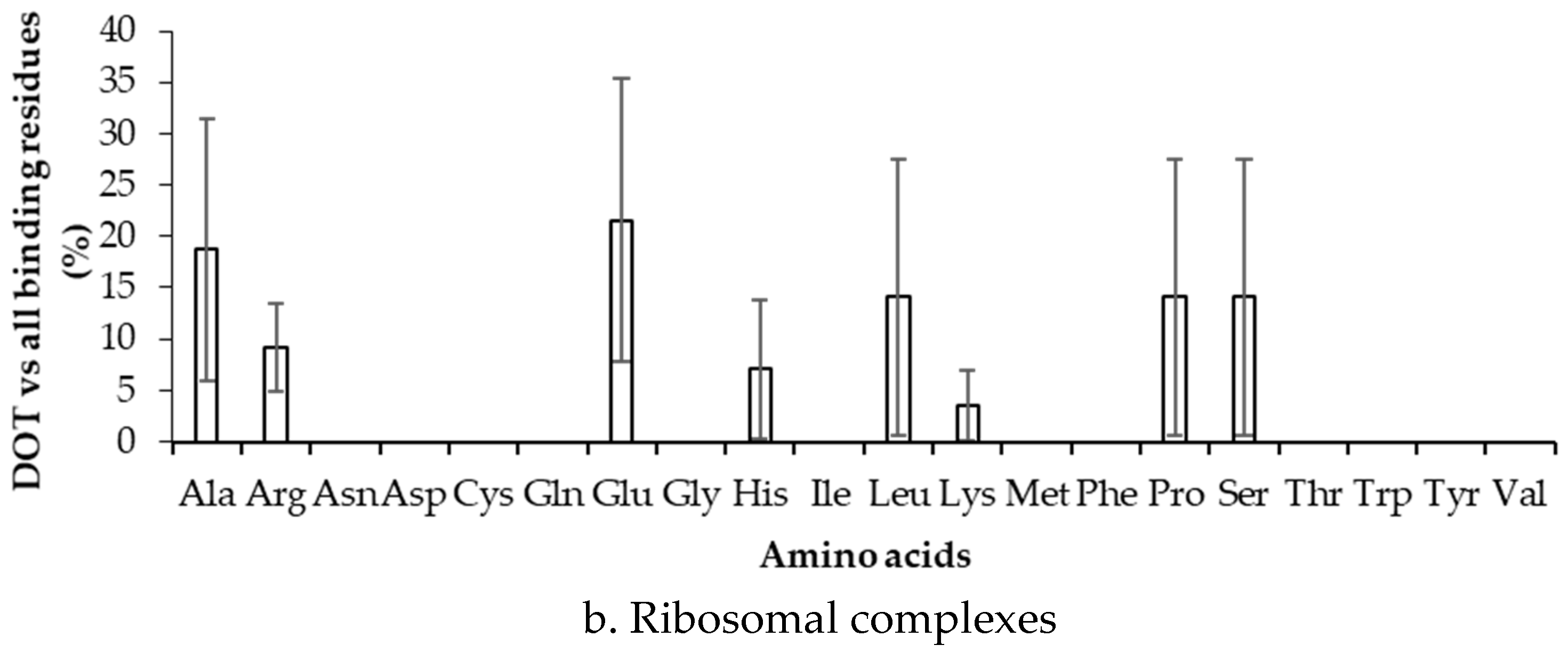
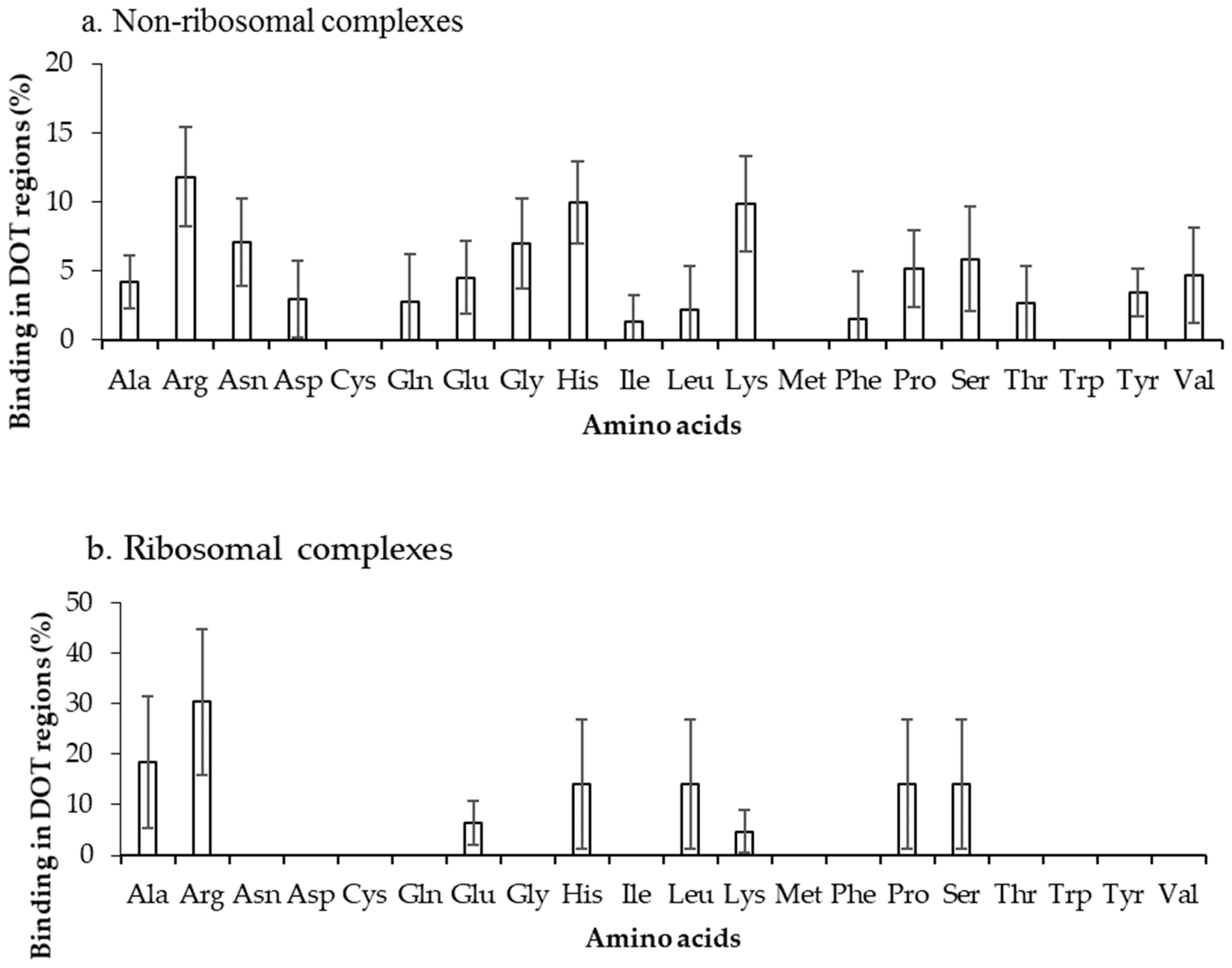
2.2. Binding Frequency of Residues at DOT Regions
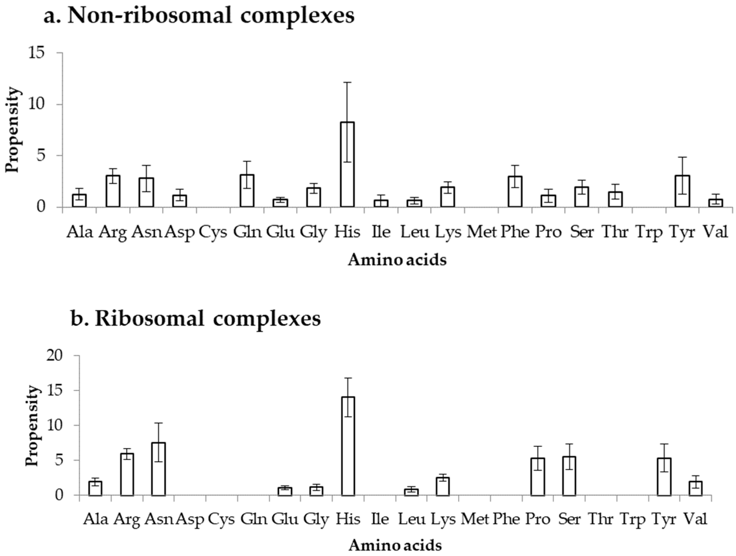
2.3. Binding Propensity of Residues at DOT Region
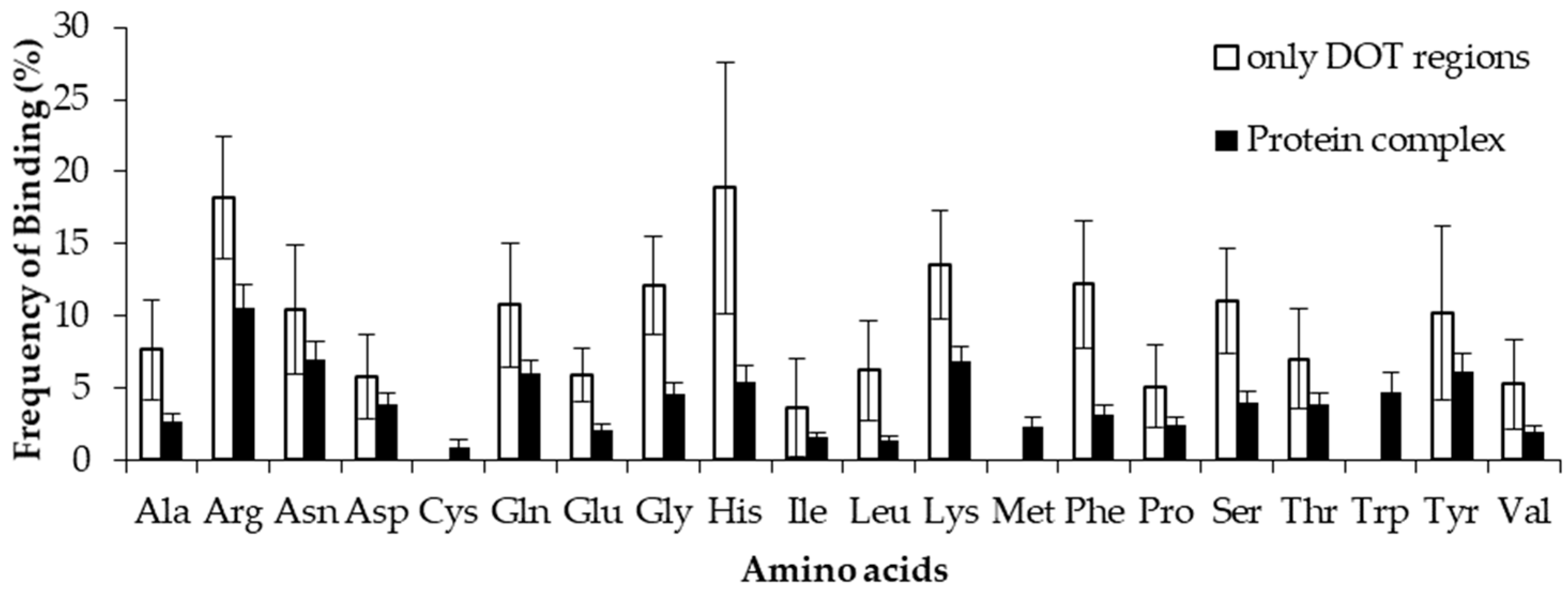
2.4. Comparison of Frequency of Binding in the DOT Region and Other Residues of a Protein
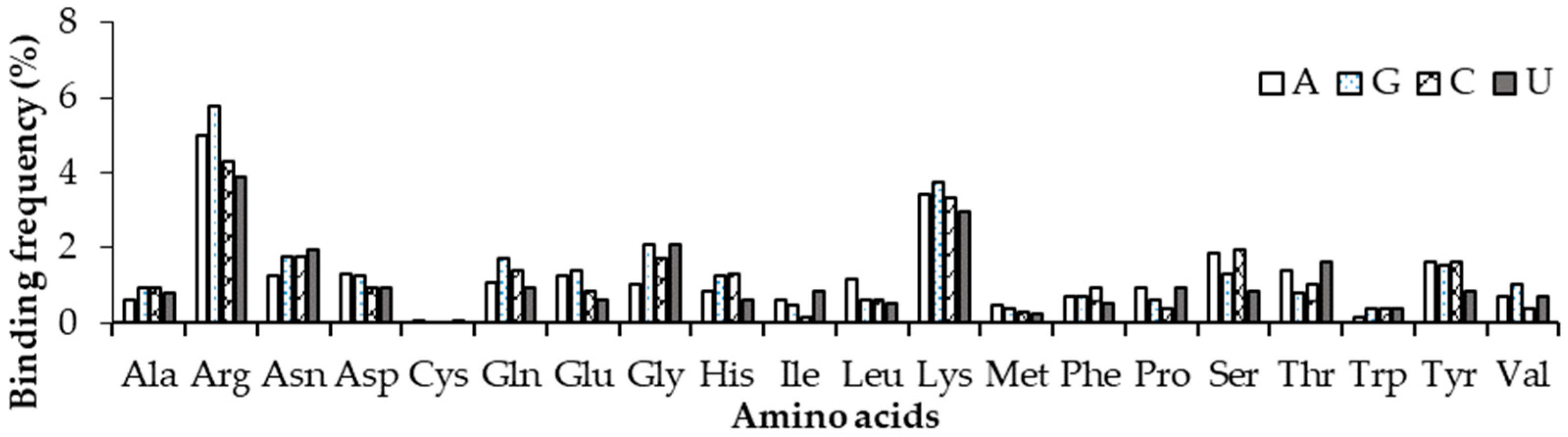
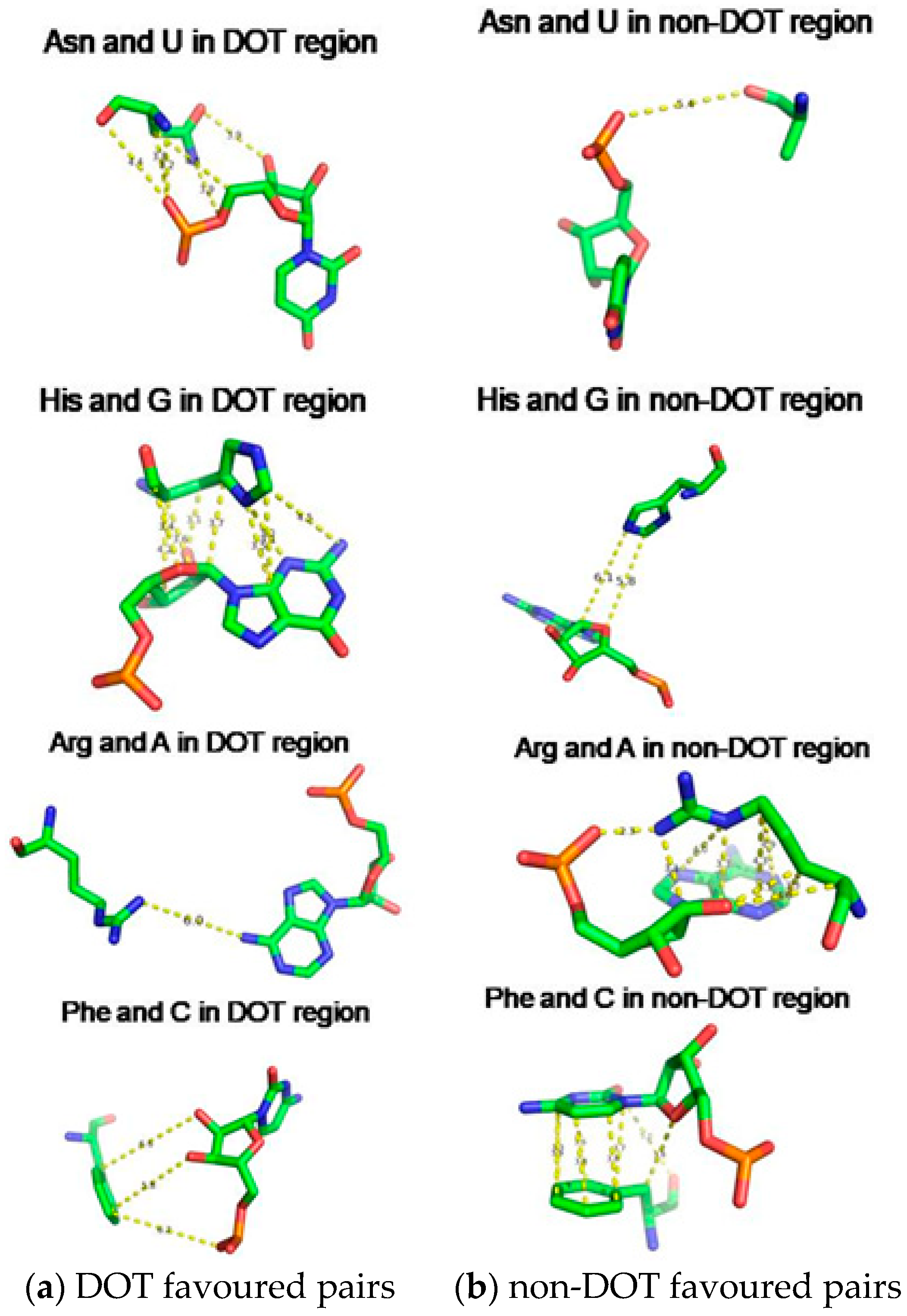
2.5. Amino Acid Contact Frequency with Nucleotides
2.6. Secondary Structure of DOT and RNA-Interacting DOT Residues
2.7. Relative Solvent Accessibility of DOT Residues
2.8. Number of Residues in Contact with Nucleotides in the DOT Region and in Entire Protein
2.9. Secondary Structure of Nucleotides Interacting with DOT Residues
2.10. Interaction Energy of DOT Residues with Nucleotides
3. Materials and Methods
3.1. Number of DOT Regions and Their Lengths
3.2. DOT Residues in Contact with RNA
3.3. Frequency of Binding in DOT and Other Residues
3.4. Propensity of Binding Residues in DOT Region
3.5. Boot Strap Sampling
3.6. Relative Average Solvent Accessibility (RASA)
3.7. Secondary Structure of Protein and RNA
3.8. Binding Preference of Nucleotides for Amino Acids
3.9. Interaction Energy between Amino Acids and Nucleotides at Binding Interface
4. Conclusions
Supplementary Materials
Author Contributions
Acknowledgments
Conflicts of Interest
References
- Habchi, J.; Tompa, P.; Longhi, S.; Uversky, V.N. Introducing protein intrinsic disorder. Chem. Rev. 2014, 114, 6561–6588. [Google Scholar] [CrossRef] [PubMed] [Green Version]
- Fuxreiter, M.; Toóth-Petroóczy, A.; Kraut, D.A.; Matouschek, A.T.; Lim, R.Y.; Xue, B.; Kurgan, L.; Uversky, V.N. Disordered proteinaceous machines. Chem. Rev. 2014, 114, 6806–6843. [Google Scholar] [CrossRef] [PubMed]
- Babu, M.M.; Van der, L.R.; de Groot, N.S.; Gsponer, J. Intrinsically disordered proteins: Regulation and disease. Curr. Opin. Struct. Biol. 2011, 21, 432–440. [Google Scholar] [CrossRef] [PubMed]
- Wright, P.E.; Dyson, H.J. Intrinsically disordered proteins in cellular signaling and regulation. Nat. Rev. Mol. Cell Biol. 2015, 16, 18–29. [Google Scholar] [CrossRef] [PubMed]
- Deller, M.C.; Kong, L.; Rupp, B. Protein stability: A crystallographer’s perspective. Acta Cryst. F 2016, 72, 72–95. [Google Scholar] [CrossRef] [PubMed]
- Johnson, D.E.; Xue, B.; Sickmeier, M.D.; Meng, J.; Cortese, M.S.; Oldfield, C.J.; Le Gall, T.; Dunker, A.K.; Uversky, V.N. High-throughput characterization of intrinsic disorder in proteins from the Protein Structure Initiative. J. Struct. Biol. 2012, 180, 201–215. [Google Scholar] [CrossRef] [PubMed]
- Dosztányi, Z.; Csizmok, V.; Tompa, P.; Simon, I. IUPred: Web server for the prediction of intrinsically unstructured regions of proteins based on estimated energy content. Bioinformatics 2005, 21, 3433–3434. [Google Scholar] [CrossRef] [PubMed]
- Jones, D.T.; Cozzetto, D. DISOPRED3: Precise disordered region predictions with annotated protein-binding activity. Bioinformatics 2014, 31, 857–863. [Google Scholar] [CrossRef] [PubMed]
- Disfani, F.M.; Hsu, W.L.; Mizianty, M.J.; Oldfield, C.J.; Xue, B.; Dunker, A.K.; Uversky, V.N.; Kurgan, L. MoRFpred, a computational tool for sequence-based prediction and characterization of short disorder-to-order transitioning binding regions in proteins. Bioinformatics 2012, 28, i75–i83. [Google Scholar] [CrossRef] [PubMed]
- Meng, F.; Uversky, V.N.; Kurgan, L. Comprehensive review of methods for prediction of intrinsic disorder and its molecular functions. Cell. Mol. Life Sci. 2017, 74, 3069–3090. [Google Scholar] [CrossRef] [PubMed]
- Berlow, R.B.; Dyson, H.J.; Wright, P.E. Functional advantages of dynamic protein disorder. FEBS Lett. 2015, 589, 2433–2440. [Google Scholar] [CrossRef] [PubMed]
- Basu, S.; Söderquist, F.; Wallner, B. Proteus: A random forest classifier to predict disorder-to-order transitioning binding regions in intrinsically disordered proteins. J. Comput. Aided Mol. Des. 2017, 31, 453–466. [Google Scholar] [CrossRef] [PubMed]
- Deane, J.E.; Ryan, D.P.; Sunde, M.; Maher, M.J.; Guss, J.M.; Visvader, J.E.; Matthews, J.M. Tandem LIM domains provide synergistic binding in the LMO4: Ldb1 complex. EMBO J. 2004, 23, 3589–3598. [Google Scholar] [CrossRef] [PubMed]
- Mark, W.Y.; Liao, J.C.; Lu, Y.; Ayed, A.; Laister, R.; Szymczyna, B.; Chakrabartty, A.; Arrowsmith, C.H. Characterization of segments from the central region of BRCA1: An intrinsically disordered scaffold for multiple protein–protein and protein–DNA interactions? J. Mol. Biol. 2005, 345, 275–287. [Google Scholar] [CrossRef] [PubMed]
- Papadakos, G.; Sharma, A.; Lancaster, L.; Bowen, R.; Kaminska, R.; Leech, A.P.; Walker, D.; Redfield, C.; Kleanthous, C. Consequences of inducing intrinsic disorder in a high-affinity protein-protein interaction. J. Am. Chem. Soc. 2015, 137, 5252–5255. [Google Scholar] [CrossRef] [PubMed]
- Fukuchi, S.; Amemiya, T.; Sakamoto, S.; Nobe, Y.; Hosoda, K.; Kado, Y.; Murakami, S.D.; Koike, R.; Hiroaki, H.; Ota, M. IDEAL in 2014 illustrates interaction networks composed of intrinsically disordered proteins and their binding partners. Nucleic Acids Res. 2014, 42, D320–D325. [Google Scholar] [CrossRef] [PubMed]
- Vacic, V.; Oldfield, C.J.; Mohan, A.; Radivojac, P.; Cortese, M.S.; Uversky, V.N.; Dunker, A.K. Characterization of molecular recognition features, MoRFs, and their binding partners. J. Proteome Res. 2007, 6, 2351–2366. [Google Scholar] [CrossRef] [PubMed]
- Sugase, K.; Dyson, H.J.; Wright, P.E. Mechanism of coupled folding and binding of an intrinsically disordered protein. Nature 2007, 447, 1021–1025. [Google Scholar] [CrossRef] [PubMed]
- Shammas, S.L.; Travis, A.J.; Clarke, J. Allostery within a transcription coactivator is predominantly mediated through dissociation rate constants. Proc. Natl. Acad. Sci. USA 2014, 111, 12055–12060. [Google Scholar] [CrossRef] [PubMed]
- Shammas, S.L.; Crabtree, M.D.; Dahal, L.; Wicky, B.I.; Clarke, J. Insights into coupled folding and binding mechanisms from kinetic studies. J. Biol. Chem. 2016, 291, 6689–6695. [Google Scholar] [CrossRef] [PubMed]
- Dyson, H.J. Roles of intrinsic disorder in protein–nucleic acid interactions. Mol. Biosyst. 2012, 8, 97–104. [Google Scholar] [CrossRef] [PubMed]
- Dey, B.; Thukral, S.; Krishnan, S.; Chakrobarty, M.; Gupta, S.; Manghani, C.; Rani, V. DNA–protein interactions: Methods for detection and analysis. Mol. Cell. Biochem. 2012, 365, 279–299. [Google Scholar] [CrossRef] [PubMed]
- Popova, V.V.; Kurshakova, M.M.; Kopytova, D.V. Methods to study the RNA-protein interactions. Mol. Biol. 2015, 49, 472–481. [Google Scholar] [CrossRef]
- Walia, R.R.; Caragea, C.; Lewis, B.A.; Towfic, F.; Terribilini, M.; El-Manzalawy, Y.; Dobbs, D.; Honavar, V. Protein–RNA interface residue prediction using machine learning: An assessment of the state of the art. BMC Bioinform. 2012, 13, 89. [Google Scholar] [CrossRef] [PubMed]
- Kumar, M.; Gromiha, M.M.; Raghava, G.P. Prediction of RNA binding sites in a protein using SVM and PSSM profile. Proteins 2008, 71, 189–194. [Google Scholar] [CrossRef] [PubMed]
- Terribilini, M.; Sander, J.D.; Lee, J.H.; Zaback, P.; Jernigan, R.L.; Honavar, V.; Dobbs, D. RNABindR: A server for analyzing and predicting RNA-binding sites in proteins. Nucleic Acids Res. 2007, 35, W578–W584. [Google Scholar] [CrossRef] [PubMed]
- Wang, L.; Brown, S.J. BindN: A web-based tool for efficient prediction of DNA and RNA binding sites in amino acid sequences. Nucleic Acids Res. 2006, 34, W243–W248. [Google Scholar] [CrossRef] [PubMed]
- Zhang, J.; Ma, Z.; Kurgan, L. Comprehensive review and empirical analysis of hallmarks of DNA-, RNA-and protein-binding residues in protein chains. Brief. Bioinform. 2017, 1–19. [Google Scholar] [CrossRef] [PubMed]
- Wang, L.; Huang, C.; Yang, M.Q.; Yang, J.Y. BindN+ for accurate prediction of DNA and RNA-binding residues from protein sequence features. BMC Syst. Biol. 2010, 4, S3. [Google Scholar] [CrossRef] [PubMed]
- Yan, J.; Friedrich, S.; Kurgan, L. A comprehensive comparative review of sequence-based predictors of DNA-and RNA-binding residues. Brief. Bioinform. 2015, 17, 88–105. [Google Scholar] [CrossRef] [PubMed]
- Tuszynska, I.; Bujnicki, J.M. DARS-RNP and QUASI-RNP: New statistical potentials for protein–RNA docking. BMC Bioinform. 2011, 12, 348. [Google Scholar] [CrossRef] [PubMed]
- Wang, Y.; Guo, Y.; Pu, X.; Li, M. A sequence-based computational method for prediction of MoRFs. RSC Adv. 2017, 7, 18937–18945. [Google Scholar] [CrossRef]
- Peng, Z.; Kurgan, L. High-throughput prediction of RNA, DNA and protein binding regions mediated by intrinsic disorder. Nucleic Acids Res. 2015, 43, e121. [Google Scholar] [CrossRef] [PubMed]
- Kim, O.T.; Yura, K.; Go, N. Amino acid residue doublet propensity in the protein–RNA interface and its application to RNA interface prediction. Nucleic Acids Res. 2006, 34, 6450–6460. [Google Scholar] [CrossRef] [PubMed]
- Mohan, A.; Oldfield, C.J.; Radivojac, P.; Vacic, V.; Cortese, M.S.; Dunker, A.K.; Uversky, V.N. Analysis of molecular recognition features (MoRFs). J. Mol. Biol. 2006, 362, 1043–1059. [Google Scholar] [CrossRef] [PubMed]
- Fernandez, M.; Kumagai, Y.; Standley, D.M.; Sarai, A.; Mizuguchi, K.; Ahmad, S. Prediction of dinucleotide-specific RNA-binding sites in proteins. BMC Bioinform. 2011, 12, S5. [Google Scholar] [CrossRef] [PubMed]
- Rose, P.W.; Prlić, A.; Altunkaya, A.; Bi, C.; Bradley, A.R.; Christie, C.H.; Costanzo, L.D.; Duarte, J.M.; Dutta, S.; Feng, Z.; Green, R.K. The RCSB protein data bank: Integrative view of protein, gene and 3D structural information. Nucleic Acids Res. 2017, 45, D271–D281. [Google Scholar] [PubMed]
- Berman, H.M.; Olson, W.K.; Beveridge, D.L.; Westbrook, J.; Gelbin, A.; Demeny, T.; Hsieh, S.H.; Srinivasan, A.R.; Schneider, B. The nucleic acid database. A comprehensive relational database of three-dimensional structures of nucleic acids. Biophys. J. 1992, 63, 751–759. [Google Scholar] [CrossRef]
- Coimbatore Narayanan, B.; Westbrook, J.; Ghosh, S.; Petrov, A.I.; Sweeney, B.; Zirbel, C.L.; Leontis, N.B.; Berman, H.M. The Nucleic Acid Database: New features and capabilities. Nucleic Acids Res. 2014, 42, D114–D122. [Google Scholar] [CrossRef] [PubMed]
- Huang, Y.; Niu, B.; Gao, Y.; Fu, L.; Li, W. CD-HIT Suite: A web server for clustering and comparing biological sequences. Bioinformatics 2010, 26, 680–682. [Google Scholar] [CrossRef] [PubMed]
- Boratyn, G.M.; Schäffer, A.A.; Agarwala, R.; Altschul, S.F.; Lipman, D.J.; Madden, T.L. Domain enhanced lookup time accelerated BLAST. Biol. Direct. 2012, 7, 12. [Google Scholar] [CrossRef] [PubMed]
- Altschul, S.F.; Gish, W.; Miller, W.; Myers, E.W.; Lipman, D.J. Basic local alignment search tool. J. Mol. Biol. 1990, 215, 403–410. [Google Scholar] [CrossRef]
- Gromiha, M.M. Protein Bioinformatics: From Sequence to Function; Academic Press: Cambridge, MA, USA, 2010. [Google Scholar]
- Si, J.; Zhao, R.; Wu, R. An overview of the prediction of protein DNA-binding sites. Int. J. Mol. Sci. 2015, 16, 5194–5215. [Google Scholar] [CrossRef] [PubMed]
- Nagarajan, R.; Gromiha, M.M. Prediction of RNA binding residues: An extensive analysis based on structure and function to select the best predictor. PLoS ONE 2014, 9, e91140. [Google Scholar] [CrossRef] [PubMed]
- Ciriello, G.; Gallina, C.; Guerra, C. Analysis of interactions between ribosomal proteins and RNA structural motifs. BMC Bioinform. 2010, 11, S41. [Google Scholar] [CrossRef] [PubMed]
- NACCESS, V2.1.1. A Computer Program for Solvent Accessible Area Calculations; Department of Biochemistry and Molecular Biology, University College London: London, UK, 1993. [Google Scholar]
- Kabsch, W.; Sander, C. Dictionary of protein secondary structure: Pattern recognition of hydrogen-bonded and geometrical features. Biopolymers 1983, 22, 2577–2637. [Google Scholar] [CrossRef] [PubMed]
- Lu, X.J.; Bussemaker, H.J.; Olson, W.K. DSSR: An integrated software tool for dissecting the spatial structure of RNA. Nucleic Acids Res. 2015, 43, e142. [Google Scholar] [CrossRef] [PubMed]
- Cornell, W.D.; Cieplak, P.; Bayly, C.I.; Gould, I.R.; Merz, K.M.; Ferguson, D.M.; Spellmeyer, D.C.; Fox, T.; Caldwell, J.W.; Kollman, P.A. A second generation force field for the simulation of proteins, nucleic acids, and organic molecules. J. Am. Chem. Soc. 1995, 117, 5179–5197. [Google Scholar] [CrossRef]
- Gromiha, M.M.; Yokota, K.; Fukui, K. Understanding the recognition mechanism of protein–RNA complexes using energy based approach. Curr. Protein Pept. Sci. 2010, 11, 629–638. [Google Scholar] [CrossRef] [PubMed]


| Secondary Structure | Number of Binding Residues in DOT Regions (Nidt) | Number of Residues in DOT Region (Nd) | Relative Binding in DOT Regions (%) |
|---|---|---|---|
| Helix | 25 (22.12) | 288 (24.51) | 8.6 |
| Sheet | 22 (19.47) | 145 (12.34) | 15.2 |
| Others (coil, turn, bend) | 66 (58.41) | 742 (63.15) | 8.9 |
| Amino Acids | RASA in DOT Regions | RASA in Complete Protein | Fold Difference |
|---|---|---|---|
| Ala | 44.743 | 23.305 | 1.920 |
| Arg | 52.168 | 40.822 | 1.278 |
| Asn | 63.583 | 42.721 | 1.488 |
| Asp | 56.552 | 43.811 | 1.291 |
| Cys | 22.32 | 11.426 | 1.953 |
| Gln | 47.805 | 38.988 | 1.226 |
| Glu | 53.688 | 47.838 | 1.122 |
| Gly | 51.599 | 35.272 | 1.463 |
| His | 43.229 | 35.372 | 1.222 |
| Ile | 26.618 | 14.692 | 1.812 |
| Leu | 32.007 | 16.374 | 1.955 |
| Lys | 58.529 | 49.520 | 1.182 |
| Met | 41.13 | 20.391 | 2.017 |
| Phe | 32.481 | 17.519 | 1.854 |
| Pro | 56.463 | 38.230 | 1.477 |
| Ser | 54.574 | 34.622 | 1.576 |
| Thr | 49.852 | 31.074 | 1.604 |
| Trp | 21.571 | 19.029 | 1.134 |
| Tyr | 44.579 | 24.752 | 1.801 |
| Val | 31.433 | 17.405 | 1.806 |
| Nucleotides | Number of Nucleotide in Contact with DOT Regions (Nidt) | Number of Nucleotides in Contact with Any Residue of Proteins (Nprot) | Relative Contact in DOT Regions (%) |
|---|---|---|---|
| A | 18 (18.75) | 137 (25.66) | 13.1 |
| C | 26 (27.08) | 131 (24.53) | 19.8 |
| G | 32 (33.33) | 157 (29.40) | 20.4 |
| U | 20 (20.83) | 109 (20.41) | 18.3 |
| Nucleotides | Secondary Structure | Number of Nucleotide in Contact with DOT Regions (Nidt) | Number of Nucleotides in Contact with Any Residue of Proteins (Nprot) | Relative Contact in DOT Regions (%) |
|---|---|---|---|---|
| A | Unpaired | 12 (12.50) | 106 (19.56) | 11.01 |
| A | Basepaired | 6 (6.25) | 30 (5.54) | 20.00 |
| A | Pseudoknot | 0 (0) | 0 (0) | 0 |
| C | Unpaired | 8 (8.33) | 70 (12.92) | 11.42 |
| C | Basepaired | 17 (17.71) | 59 (10.89) | 28.81 |
| C | Pseudoknot | 1 (1.04) | 5 (0.92) | 20.00 |
| G | Unpaired | 16 (16.67) | 87 (16.05) | 18.39 |
| G | Basepaired | 15 (15.63) | 71 (13.10) | 21.13 |
| G | Pseudoknot | 1 (1.04) | 4 (0.74) | 25.00 |
| U | Unpaired | 15 (15.63) | 81 (14.94) | 18.51 |
| U | Basepaired | 5 (5.21) | 29 (5.35) | 17.24 |
| U | Pseudoknot | 0 (0) | 0 (0) | 0 |
| All | Unpaired | 51 (53.13) | 344 (63.47) | 14.83 |
| All | Basepaired | 43 (44.79) | 189 (34.87) | 22.75 |
| All | Pseudoknot | 2 (2.08) | 9 (1.66) | 22.22 |
| Amino Acids | A | G | C | U |
|---|---|---|---|---|
| Ala | −0.62 (−0.55) | −0.34 (−0.57) | −0.49 (−0.53) | −0.55 (−0.64) |
| Arg | −0.36 (−1.23) | −1.15 (−0.83) | −0.89 (−0.95) | −1.06 (−0.98) |
| Asn | −0.45 (−0.68) | −0.59 (−0.73) | −0.48 (−0.83) | −1.85 (−0.82) |
| Asp | −0.75 (−0.74) | −0.39 (−0.79) | −0.19 (−0.56) | −1.40 (−0.92) |
| Cys | 0.00 (−0.87) | −0.01 (−0.03) | −0.03 (−1.10) | −0.63 (−1.13) |
| Gln | −0.15 (−0.87) | −0.57 (−0.74) | −0.08 (−0.84) | −0.36 (−0.71) |
| Glu | −0.72 (−0.80) | −0.41 (−0.64) | −0.43 (−0.62) | −0.68 (−0.59) |
| Gly | −0.28 (−0.47) | −0.37 (−0.69) | −0.58 (−0.57) | −1.07 (−0.79) |
| His | −0.81 (−1.17) | −2.13 (−1.41) | −1.53 (−1.21) | −0.70 (−1.01) |
| Ile | −0.60 (−0.64) | −1.63 (−0.80) | −0.54 (−0.50) | −1.33 (−0.76) |
| Leu | −0.35 (−0.75) | −1.19 (−0.50) | −0.42 (−0.49) | −0.54 (−0.41) |
| Lys | −0.74 (−0.76) | −0.86 (−0.83) | −0.66 (−0.90) | −0.83 (−0.83) |
| Met | −0.64 (−1.05) | −0.07 (−0.75) | −0.16 (−1.03) | −0.83 (−1.19) |
| Phe | −0.81 (−1.03) | −1.12 (−0.89) | −0.54 (−1.32) | −0.24 (−1.42) |
| Pro | −0.88 (−0.83) | −0.60 (−0.88) | −0.62 (−0.91) | −0.69 (−1.00) |
| Ser | −0.79 (−0.77) | −0.29 (−0.56) | −1.24 (−0.71) | −1.41 (−0.68) |
| Thr | −0.39 (−0.68) | −0.66 (−0.56) | −0.67 (−0.64) | −0.53 (−1.00) |
| Trp | −1.15 (−1.10) | 0.00 (−1.64) | 0.00 (−0.99) | 0.00 (−1.34) |
| Tyr | −1.53 (−1.36) | −1.11 (−1.42) | −0.63 (−1.05) | −0.16 (−1.09) |
| Val | −0.38 (−0.70) | −0.66 (−0.53) | −0.64 (−0.53) | −0.52 (−0.76) |
© 2018 by the authors. Licensee MDPI, Basel, Switzerland. This article is an open access article distributed under the terms and conditions of the Creative Commons Attribution (CC BY) license (http://creativecommons.org/licenses/by/4.0/).
Share and Cite
Srivastava, A.; Ahmad, S.; Gromiha, M.M. Deciphering RNA-Recognition Patterns of Intrinsically Disordered Proteins. Int. J. Mol. Sci. 2018, 19, 1595. https://doi.org/10.3390/ijms19061595
Srivastava A, Ahmad S, Gromiha MM. Deciphering RNA-Recognition Patterns of Intrinsically Disordered Proteins. International Journal of Molecular Sciences. 2018; 19(6):1595. https://doi.org/10.3390/ijms19061595
Chicago/Turabian StyleSrivastava, Ambuj, Shandar Ahmad, and M. Michael Gromiha. 2018. "Deciphering RNA-Recognition Patterns of Intrinsically Disordered Proteins" International Journal of Molecular Sciences 19, no. 6: 1595. https://doi.org/10.3390/ijms19061595
APA StyleSrivastava, A., Ahmad, S., & Gromiha, M. M. (2018). Deciphering RNA-Recognition Patterns of Intrinsically Disordered Proteins. International Journal of Molecular Sciences, 19(6), 1595. https://doi.org/10.3390/ijms19061595