In Silico Prediction of Estrogen Receptor Subtype Binding Affinity and Selectivity Using Statistical Methods and Molecular Docking with 2-Arylnaphthalenes and 2-Arylquinolines

Abstract
:1. Introduction
2. Material and Methods
2.1. The Data Set
2.2. Molecular Descriptors
2.3. Statistical Methods
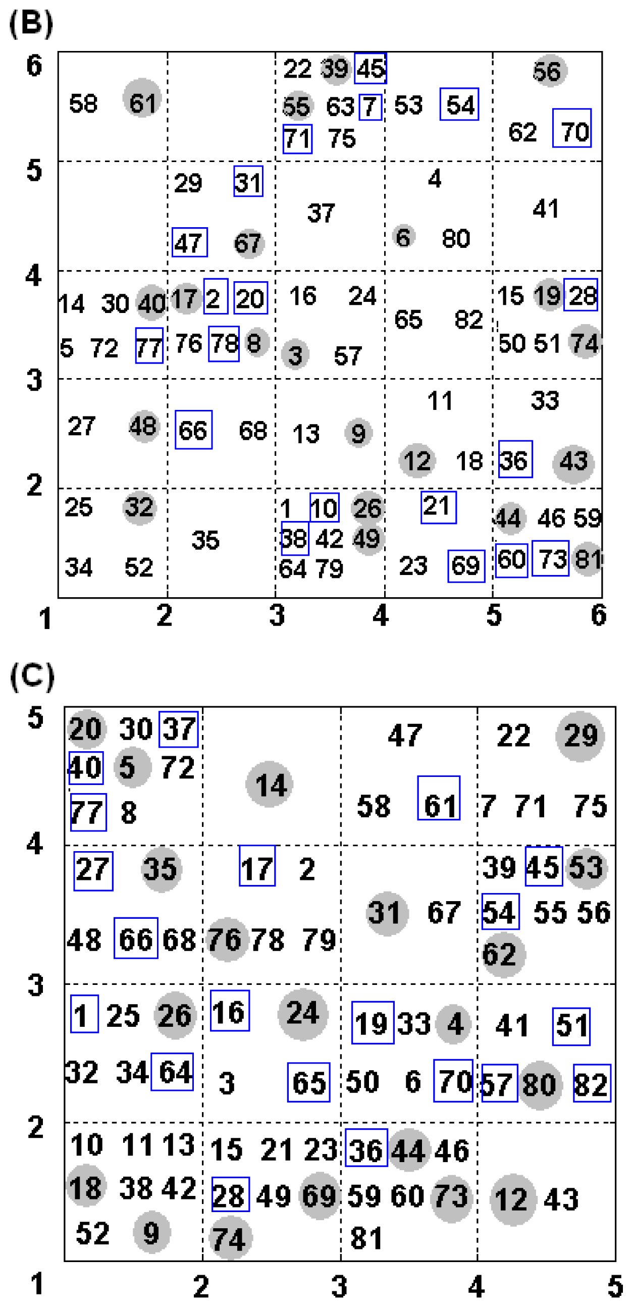
2.4. Construction of Training and Test Set
2.5. Docking
3. Results
3.1. ERα
3.1.1. MLR
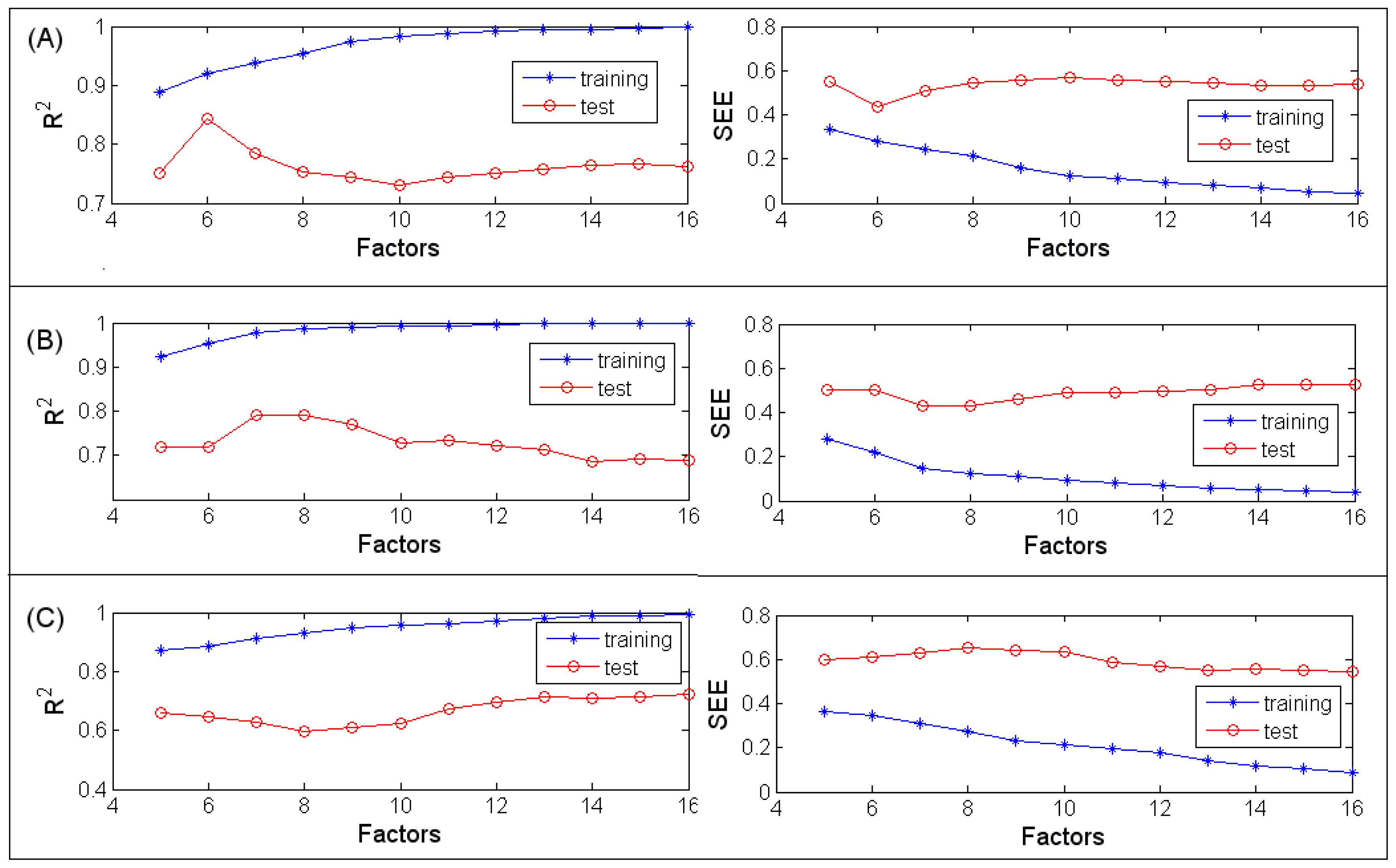
3.1.2. PLSR
3.1.3. BRNN
3.1.4. Surflex-Docking
3.2. ERβ
3.2.1. MLR
3.2.2. PLSR
3.2.3. BRNN
3.2.4. Surflex-Dock
3.3. Selectivity
3.3.1. MLR
3.3.2. PLSR
3.3.3. BRNN
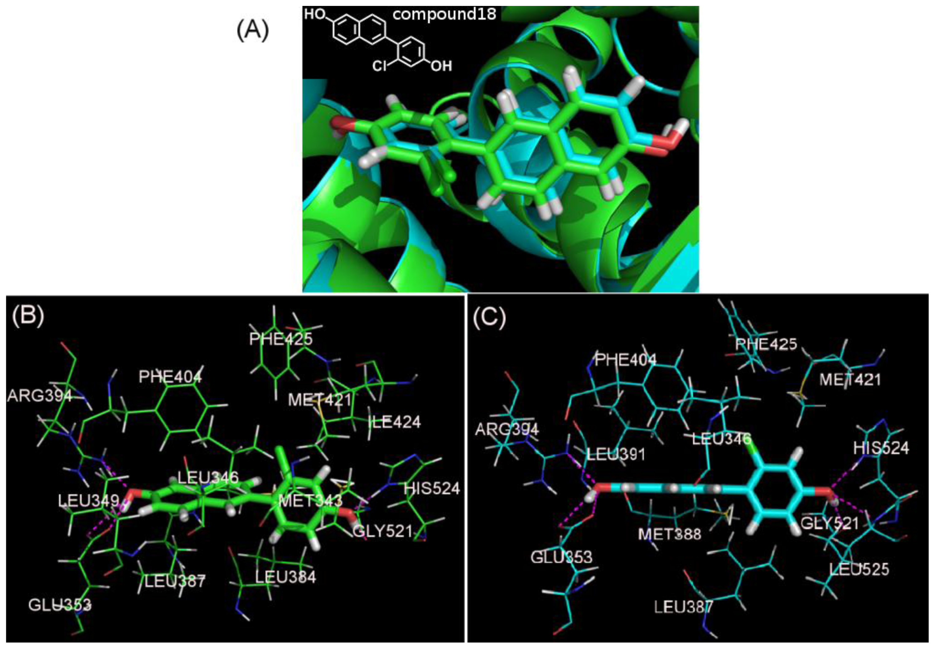
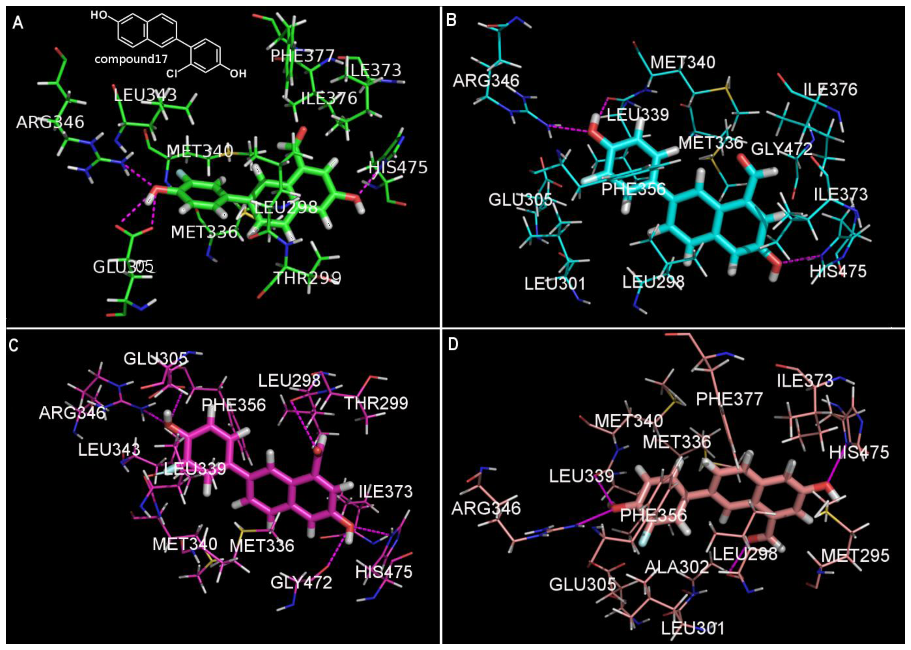
3.3.4. Docking Study
4. Discussion
4.1 ERα Models
4.2. ERβ Models
4.3. Selectivity Models
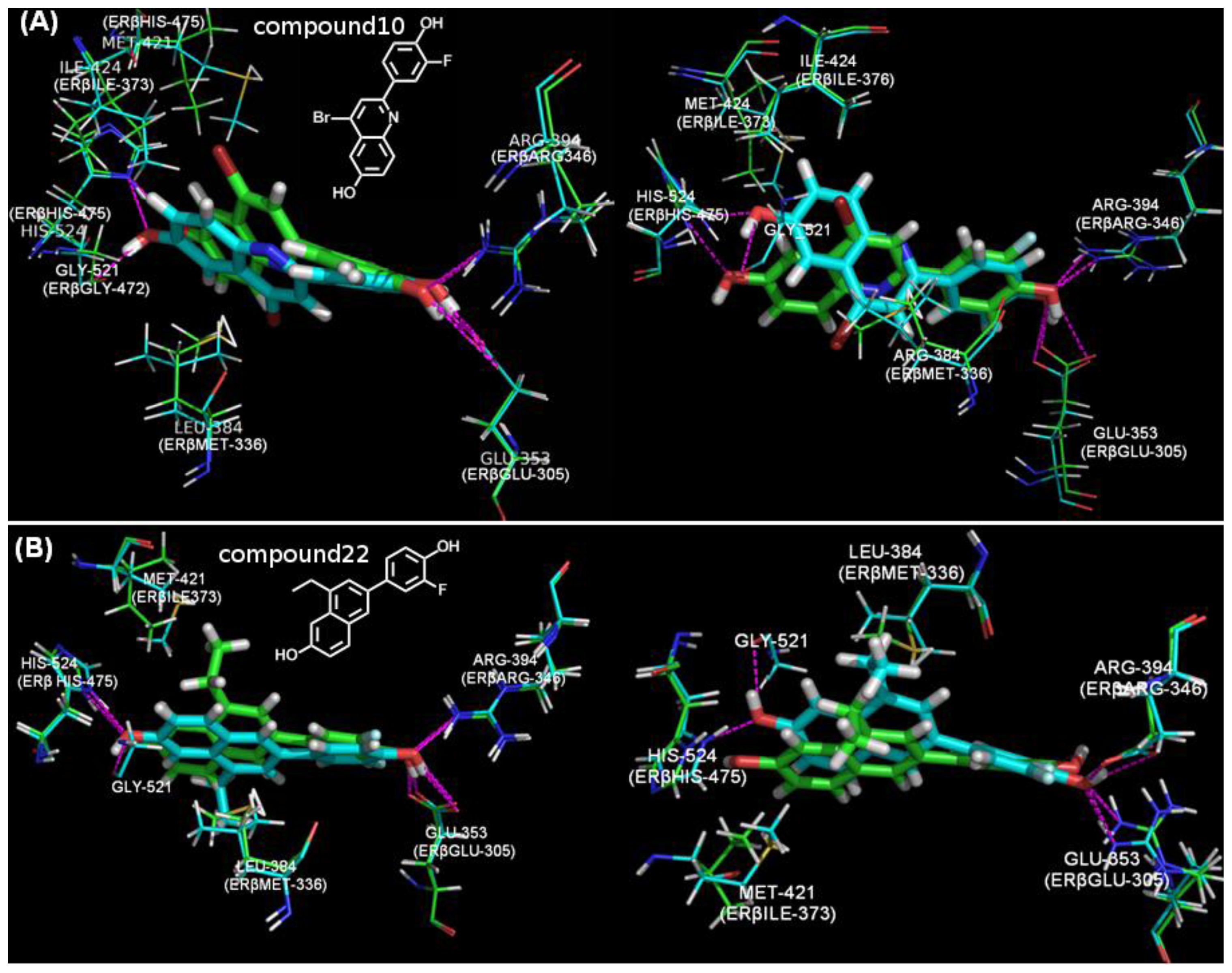
4.4. The Docking Study
5. Conclusions
References
- Gronemeyer, H; Gustafsson, JA; Laudet, V. Principles for modulation of the nuclear receptor superfamily. Nat. Rev. Drug Discov 2004, 3, 950–964. [Google Scholar]
- Horwitz, KB; Jackson, TA; Bain, DL; Richer, JK; Takimoto, GS; Tung, L. Nuclear receptor coactivators and corepressors. Mol. Endocrinol 1996, 10, 1167–1177. [Google Scholar]
- Nilsson, S; Gustafsson, JA. Biological role of estrogen and estrogen receptors. Crit. Rev. Biochem. Mol. Biol 2002, 37, 1–28. [Google Scholar]
- Fitzpatrick, SL; Funkhouser, JM; Sindoni, DM; Stevis, PE; Deecher, DC; Bapat, AR; Merchenthaler, I; Frail, DE. Expression of estrogen receptor-beta protein in rodent ovary. Endocrinology 1999, 140, 2581–2591. [Google Scholar]
- Kuiper, GG; Carlsson, B; Grandien, K; Enmark, E; Haggblad, J; Nilsson, S; Gustafsson, JA. Comparison of the ligand binding specificity and transcript tissue distribution of estrogen receptors alpha and beta. Endocrinology 1997, 138, 863–870. [Google Scholar]
- Minutolo, F; Macchia, M; Katzenellenbogen, BS; Katzenellenbogen, JA. Estrogen receptor beta ligands: Recent advances and biomedical applications. Med. Res. Rev 2010. [Google Scholar] [CrossRef]
- Zhao, LQ; Brinton, RD. Estrogen receptor beta as a therapeutic target for promoting neurogenesis and preventing neurodegeneration. Drug Dev. Res 2005, 66, 103–117. [Google Scholar]
- Mortensen, DS; Rodriguez, AL; Sun, J; Katzenellenbogen, BS; Katzenellenbogen, JA. Furans with basic side chains: Synthesis and biological evaluation of a novel series of antagonists with selectivity for the estrogen receptor alpha. Bioorg. Med. Chem. Lett 2001, 11, 2521–2524. [Google Scholar]
- Mewshaw, RE; Edsall, RJ; Yang, CJ; Manas, ES; Xu, ZB; Henderson, RA; Keith, JC; Harris, HA. ER beta ligands. 3. Exploiting two binding orientations of the 2-phenylnaphthalene scaffold to achieve ER beta selectivity. J. Med. Chem 2005, 48, 3953–3979. [Google Scholar]
- Gungor, T; Chen, Y; Golla, R; Ma, Z; Corte, JR; Northrop, JP; Bin, B; Dickson, JK; Stouch, T; Zhou, R; Johnson, SE; Seethala, R; Feyen, JH. Synthesis and characterization of 3-arylquinazolinone and 3-arylquinazolinethione derivatives as selective estrogen receptor beta modulators. J. Med. Chem 2006, 49, 2440–2455. [Google Scholar]
- Minutolo, F; Bellini, R; Bertini, S; Carboni, I; Lapucci, A; Pistolesi, L; Prota, G; Rapposelli, S; Solati, F; Tuccinardi, T; Martinelli, A; Stossi, F; Carlson, KE; Katzenellenbogen, BS; Katzenellenbogen, JA; Macchia, M. Monoaryl-substituted salicylaldoximes as ligands for estrogen receptor beta. J. Med. Chem 2008, 51, 1344–1351. [Google Scholar]
- Xu, X; Yang, W; Li, Y; Wang, YH. Discovery of estrogen receptor modulators: A review of virtual screening and SAR efforts. Exp. Opin. Drug Disc 2010, 5, 21–31. [Google Scholar]
- Waller, CL; Oprea, TI; Chae, K; Park, HK; Korach, KS; Laws, SC; Wiese, TE; Kelce, WR; Gray, LE, Jr. Ligand-based identification of environmental estrogens. Chem. Res. Toxicol 1996, 9, 1240–1248. [Google Scholar]
- Asikainen, AH; Ruuskanen, J; Tuppurainen, KA. Consensus kNN QSAR: A versatile method for predicting the estrogenic activity of organic compounds in silico. A comparative study with five estrogen receptors and a large, diverse set of ligands. Environ. Sci. Technol 2004, 38, 6724–6729. [Google Scholar]
- Shi, LM; Fang, H; Tong, WD; Wu, J; Perkins, R; Blair, RM; Branham, WS; Dial, SL; Moland, CI; Sheehan, DM. QSAR models using a large diverse set of estrogens. J. Chem. Inf. Comput. Sci 2001, 41, 186–195. [Google Scholar]
- Wolohan, P; Reichert, DE. CoMFA and docking study of novel estrogen receptor subtype selective ligands. J. Comput.-Aided Mol. Des 2003, 17, 313–328. [Google Scholar]
- Agatonovic-Kustrin, S; Turner, JV; Glass, BD. Molecular structural characteristics as determinants of estrogen receptor selectivity. J. Pharm. Biomed. Anal 2008, 48, 369–375. [Google Scholar]
- Barrett, I; Meegan, MJ; Hughes, RB; Carr, M; Knox, AJ; Artemenko, N; Golfis, G; Zisterer, DM; Lloyd, DG. Synthesis, biological evaluation, structural-activity relationship, and docking study for a series of benzoxepin-derived estrogen receptor modulators. Bioorg. Med. Chem 2008, 16, 9554–9573. [Google Scholar]
- Kim, KH; Greco, G; Novellino, E. A critical review of recent CoMFA applications. In Perspectives in Drug Discovery and Design; Sprigner: Dordrecht, The Netherlands, 1998; pp. 257–315. [Google Scholar]
- Sutherland, JJ; O’Brien, LA; Weaver, DF. A comparison of methods for modeling quantitative structure-activity relationships. J. Med. Chem 2004, 47, 5541–5554. [Google Scholar]
- Ghafourian, T; Cronin, MT. The impact of variable selection on the modelling of oestrogenicity. SAR QSAR Environ. Res 2005, 16, 171–190. [Google Scholar]
- Mackay, DJC. Probable networks and plausible predictions - a review of practical bayesian methods for supervised neural networks. Netw.-Comput. Neural. Syst 1995, 6, 469–505. [Google Scholar]
- Wang, YH; Li, Y; Yang, SL; Yang, L. An in silico approach for screening flavonoids as P-glycoprotein inhibitors based on a Bayesian-regularized neural network. J. Comput.-Aided Mol. Design 2005, 19, 137–147. [Google Scholar]
- Vu, AT; Cohn, ST; Manas, ES; Harris, HA; Mewshaw, RE. ER beta ligands. Part 4: Synthesis and structure-activity relationships of a series of 2-phenylquinoline derivatives. Bioorg. Med. Chem. Lett 2005, 15, 4520–4525. [Google Scholar]
- Wang, YH; Li, Y; Ding, J; Wang, Y; Chang, YQ. Prediction of binding affinity for estrogen receptor(alpha) modulators using statistical learning approaches. Mol. Divers 2008, 12, 93–102. [Google Scholar]
- Geladi, P; Kowalski, BR. Partial least-squares regression: A tutorial. Anal. Chim. Acta 1986, 185, 1–17. [Google Scholar]
- Rosipal, R; Kramer, N. Saunders, C, Grobelnik, M, Gunn, SR, Shawe-Taylor, J, Eds.; Overview and recent advances in partial least squares. In Subspace, Latent Structure and Feature Selection; Springer: New York, NY, USA, 2006; pp. 34–51. [Google Scholar]
- Caballero, J; Fernandez, M. Linear and nonlinear modeling of antifungal activity of some heterocyclic ring derivatives using multiple linear regression and Bayesian-regularized neural networks. J. Mol. Model 2006, 12, 168–181. [Google Scholar]
- Crucianu, M; Bone, R; de Beauville, JPA. Bayesian learning for recurrent neural networks. Neuralocomputing 2001, 36, 235–242. [Google Scholar]
- Mackay, DJC. Bayesian Interpolation. Neural Comput 1992, 4, 415–447. [Google Scholar]
- Foresee, FD; Hagan, MT. Gauss Newton approximation to Bayesian regularization. Proceedings of the 1997 International Joint Conference on Neural Networks, Houston, TX, USA, 9–12 June, 1997.
- Hagan, MT; Menhaj, MB. Training feedforward networks with the Marquardt algorithm. IEEE Trans. Neural Netw 1994, 5, 989–993. [Google Scholar]
- Nguyen, D; Widrow, B. Improving the learning speed of 2-layer neural networks by choosing initial values of the adaptive weights. 1990 IJCNN International Joint Conference on Neural Networks, Washington, DC, USA, 17–21 June, 1990.
- Mackay, DJC. A practical bayesian framework for backpropagation networks. Neural Comput 1992, 4, 448–472. [Google Scholar]
- Kohonen, T; Somervuo, P. Self-organizing maps of symbol strings. Neuralocomputing 1998, 21, 19–30. [Google Scholar]
- Wang, YH; Han, KL; Yang, SL; Yang, L. Structural determinants of steroids for cytochrome P450–3A4-mediated metabolism. J. Mol. Struct.-Theochem 2004, 710, 215–221. [Google Scholar]
- Jain, AN. Surflex: Fully automatic flexible molecular docking using a molecular similarity-based search engine. J. Med. Chem 2003, 46, 499–511. [Google Scholar]
- Jain, AN. Surflex-Dock 2.1: Robust performance from ligand energetic modeling, ring flexibility, and knowledge-based search. J. Comput.-Aided Mol. Design 2007, 21, 281–306. [Google Scholar]
- Pike, AC; Brzozowski, AM; Hubbard, RE; Bonn, T; Thorsell, AG; Engstrom, O; Ljunggren, J; Gustafsson, JA; Carlquist, M. Structure of the ligand-binding domain of oestrogen receptor beta in the presence of a partial agonist and a full antagonist. EMBO J 1999, 18, 4608–4618. [Google Scholar]
- Salum, LB; Polikarpov, I; Andricopulo, AD. Structure-based approach for the study of estrogen receptor binding affinity and subtype selectivity. J. Chem. Inf. Model 2008, 48, 2243–2253. [Google Scholar]
- Todeschini, R; Consonni Mannhold, R; Kubinyi, H; Timmerman, H. Handbook of Molecule Descriptors; Wiley-VCH: Weinheim, Germany, 2000. [Google Scholar]
- Feher, M; Williams, CI. Effect of input differences on the results of docking calculations. J. Chem. Inf. Model 2009, 49, 1704–1714. [Google Scholar]
- Wolohan, P; Reichert, DE. CoMFA and docking study of novel estrogen receptor subtype selective ligands. J. Comput. Aided Mol. Des 2003, 17, 313–328. [Google Scholar]
- Mukherjee, S; Nagar, S; Mullick, S; Mukherjee, A; Saha, A. Pharmacophore mapping of selective binding affinity of estrogen modulators through classical and space modeling approaches: Exploration of bridged-cyclic compounds with diarylethylene linkage. J. Chem. Inf. Model 2007, 47, 475–487. [Google Scholar]
- Kekenes-Huskey, PM; Muegge, I; von Rauch, M; Gust, R; Knapp, EW. A molecular docking study of estrogenically active compounds with 1,2-diarylethane and 1,2-diarylethene pharmacophores. Bioorg. Med. Chem 2004, 12, 6527–6537. [Google Scholar]
- Liao, SY; Qian, L; Miao, TF; Lu, HL; Zheng, KC. CoMFA and docking studies of 2-phenylindole derivatives with anticancer activity. Eur. J. Med. Chem 2009, 44, 2822–2827. [Google Scholar]
- Yang, JM; Chen, YF; Shen, TW; Kristal, BS; Hsu, DF. Consensus scoring criteria for improving enrichment in virtual screening. J. Chem. Inf. Model 2005, 45, 1134–1146. [Google Scholar]


| NO. | SMILES | pIC50(α) | pIC50(β) | S |
|---|---|---|---|---|
| compound1 | OC1=CC=C(C2=CC(F)=C(C(Cl)=C(O)C=C3)C3=C2)C=C1 | 6.40 | 7.96 | 1.55 |
| compound2 | OC1=C(F)C=C(C2=CC=C(C=C(O)C=C3C#C)C3=C2)C=C1 | 6.14 | 7.92 | 1.78 |
| compound3 | OC1=C(F)C=C(C2=CC=C(C=C(O)C=C3F)C3=C2)C=C1 | 6.68 | 7.82 | 1.11 |
| compound4 | OC1=CC=C(C2=CC=C(C=C(O)C=C3C#N)C3=C2)C=C1 | 6.08 | 7.70 | 1.61 |
| compound5 | OC1=CC(F)=C(C2=CC=C(C=C(O)C=C3C#N)C3=C2)C(F)=C1 | 6.35 | 7.66 | 1.29 |
| compound6 | OC1=CC=C(C2=CC(C#N)=C(C=C(O)C=C3)C3=C2)C=C1 | 5.98 | 7.64 | 1.65 |
| compound7 | OC1=CC=C(C2=CC(CC)=C(C=C(O)C=C3)C3=C2)C=C1F | 5.95 | 7.60 | 1.65 |
| compound8 | OC1=CC=C(C2=CC(C#N)=C(C=C(O)C=C3)C3=C2)C=C1F | 5.68 | 7.57 | 1.89 |
| compound9 | OC1=CC=C(C2=CC=C3C(Cl)=C(O)C=CC3=C2)C(Cl)=C1 | 6.44 | 7.48 | 1.00 |
| compound10 | BrC2=CC(C3=CC=C(O)C(F)=C3)=NC1=CC=C(O)C=C12 | 5.55 | 7.47 | 1.92 |
| compound11 | BrC2=CC(C3=CC=C(O)C=C3)=NC1=CC=C(O)C=C12 | 5.67 | 7.37 | 1.68 |
| compound12 | ClC2=CC(C3=CC=C(O)C=C3)=NC1=CC=C(O)C=C12 | 5.67 | 7.34 | 1.66 |
| compound13 | ClC2=CC(C3=CC=C(O)C(F)=C3)=NC1=CC=C(O)C=C12 | 5.61 | 7.28 | 1.66 |
| compound14 | OC3=CC=C(C=C3F)C2=CC=C(C1=C2)C(C)=C(C=C1C#N)O | 5.39 | 7.22 | 1.82 |
| compound15 | OC3=CC=C(C=C3)C2=CC=C1C(F)=C(C=CC1=C2)O | 6.11 | 7.15 | 1.00 |
| compound16 | OC3=C(F)C=C(C=C3F)C2=CC=C1C=C(C=CC1=C2)O | 6.04 | 7.08 | 1.00 |
| compound17 | OC1=C(C=C(C3=CC=C2C=C(O)C=C(C2=C3)C=O)C=C1)F | 6.14 | 7.96 | 1.82 |
| compound18 | OC1=CC=C(C2=CC=C3C=C(O)C=CC3=C2)C(Cl)=C1 | 7.00 | 7.85 | 0.79 |
| compound19 | OC3=CC=C(C=C3)C2=CC(F)=C1C=C(C=CC1=C2)O | 6.66 | 7.80 | 1.11 |
| compound20 | OC3=C(F)C=C(C=C3)C2=CC=C1C=C(C=C(C#N)C1=C2)O | 6.02 | 7.68 | 1.65 |
| compound21 | OC3=CC=C(C=C3)C2=CC(Cl)=C1C=C(C=CC1=C2)O | 6.52 | 7.64 | 1.08 |
| compound22 | OC3=CC=C(C=C3F)C2=CC(CC)=C1C=C(C=CC1=C2)O | 5.63 | 7.62 | 1.99 |
| compound23 | OC3=CC=C(C=C3)C2=CC=C1C(Cl)=C(C=CC1=C2)O | 6.04 | 7.60 | 1.55 |
| compound24 | OC3=C(F)C=C(C(F)=C3)C2=CC=C1C=C(C=CC1=C2)O | 6.57 | 7.55 | 0.94 |
| compound25 | OC3=CC(F)=C(C(F)=C3)C2=CC=C1C(Cl)=C(C=CC1=C2)O | 6.46 | 7.47 | 0.97 |
| compound26 | OC3=CC=C(C=C3F)C2=CC=C1C(Cl)=C(C=CC1=C2)O | 5.84 | 7.40 | 1.54 |
| compound27 | OC3=C(F)C=C(C=C3)C2=CC=C1C(Br)=C(C=C(C#N)C1=C2)O | 5.94 | 7.35 | 1.39 |
| compound28 | OC3=CC=C(C=C3F)C2=CC=C1C=C(C=CC1=C2)O | 6.04 | 7.30 | 1.24 |
| compound29 | OC3=C(F)C=C(C=C3)C2=CC=C1C=C(C=C(C#CC)C1=C2)O | 5.74 | 7.26 | 1.50 |
| compound30 | OC3=C(F)C=C(C(F)=C3)C2=CC(C#N)=C1C=C(C=CC1=C2)O | 5.73 | 7.16 | 1.41 |
| compound31 | OC3=C(F)C=C(C=C3)C2=CC=C1C=C(C=C(C=C)C1=C2)O | 5.28 | 7.14 | 1.85 |
| compound32 | OC3=C(F)C=C(C(F)=C3)C2=CC=C1C(Cl)=C(C=CC1=C2)O | 5.93 | 7.07 | 1.11 |
| compound33 | OC3=CC=C(C(C)=C3)C2=CC=C1C=C(C=CC1=C2)O | 6.40 | 7.00 | 0.48 |
| compound34 | OC3=C(F)C=C(C=C3F)C2=CC=C1C(Cl)=C(C=CC1=C2)O | 5.28 | 6.97 | 1.68 |
| compound35 | OC3=CC=C(C=C3)C2=CC(C#N)=C1C(Br)=C(C=CC1=C2)O | 5.88 | 6.92 | 1.00 |
| compound36 | OC3=CC=C(C=C3)C2=CC=C1C=C(C=CC1=C2)O | 5.68 | 6.79 | 1.08 |
| compound37 | OC1=CC=C2C(C(C#N)=CC(C3=CC=C(O)C(F)=C3)=N2)=C1 | 4.98 | 6.64 | 1.65 |
| compound38 | OC3=CC=C(C=C3Cl)C2=CC=C1C(Cl)=C(C=CC1=C2)O | 5.45 | 6.49 | 1.01 |
| compound39 | OC1=CC=C2C(C(C=C)=CC(C3=CC=C(O)C(F)=C3)=N2)=C1 | 5.41 | 6.36 | 0.89 |
| compound40 | OC3=C(F)C=C(C=C3F)C2=CC(C#N)=C1C=C(C=CC1=C2)O | 5.26 | 6.24 | 0.93 |
| compound41 | OC1=CC=C2C(C(C#C)=CC(C3=CC=C(O)C=C3)=N2)=C1 | 4.82 | 6.12 | 1.28 |
| compound42 | OC1=CC=C2C(C=CC(C3=CC=C(O)C=C3)=N2)=C1Br | 4.94 | 6.06 | 1.08 |
| compound43 | OC1=CC=C2C(C=CC(C3=CC=C(O)C=C3)=N2)=C1 | 4.75 | 5.77 | 0.97 |
| compound44 | OC1=CC=CC2=CC(C3=CC=CC(O)=C3)=CC=C12 | 4.84 | 5.69 | 0.78 |
| compound45 | OC1=CC=C2C(C(C(C)=O)=CC(C3=CC=C(O)C=C3)=N2)=C1 | 4.50 | 5.66 | 1.12 |
| compound46 | OC(C=CC2=C3)=CC2=CC=C3C1=CC=CC=C1 | 4.87 | 5.43 | 0.41 |
| compound47 | OC(C=CC2=C3)=CC2=C(C#CC)C=C3C1=CC=C(O)C(F)=C1 | 5.46 | 7.00 | 1.52 |
| compound48 | OC(C=CC2=C3)=C(Cl)C2=C(C#N)C=C3C1=CC=C(O)C(F)=C1 | 5.52 | 6.96 | 1.42 |
| compound49 | OC(C=CC2=C3)=C(Br)C2=CC=C3C1=CC=C(O)C=C1 | 5.58 | 6.89 | 1.29 |
| compound50 | OC(C=CC2=C3)=C(C)C2=CC=C3C1=CC=C(O)C=C1 | 5.55 | 6.77 | 1.19 |
| compound51 | OC1=CC=C2C(C=CC(C3=CC=C(O)C=C3)=N2)=C1 | 5.20 | 6.52 | 1.30 |
| compound52 | OC1=CC=C2C(C(Br)=CC(C3=CC(F)=C(O)C(F)=C3)=N2)=C1 | 5.11 | 6.44 | 1.32 |
| compound53 | OC1=CC=C2C(C(CC)=CC(C3=CC=C(O)C=C3)=N2)=C1 | 5.20 | 6.28 | 1.05 |
| compound54 | OC1=CC=C2C(C(C=C)=CC(C3=CC=C(O)C=C3)=N2)=C1 | 5.30 | 6.22 | 0.87 |
| compound55 | OC1=CC=C2C(C(CC)=CC(C3=CC=C(O)C(F)=C3)=N2)=C1 | 4.76 | 6.10 | 1.33 |
| compound56 | OC(C=CC2=C3)=C(OC)C2=CC=C3C1=CC=C(O)C=C1 | 5.05 | 5.94 | 0.83 |
| compound57 | OC(C=CC2=C3)=C( [N+]( [O−])=O)C2=CC=C3C1=CC=C(O)C=C1 | 5.15 | 5.70 | 0.41 |
| compound58 | OC1=CC=C2C(C(C4=CC=CC=C4)=CC(C3=CC=C(O)C(F)=C3)=N2)=C1 | 4.74 | 5.68 | 0.88 |
| compound59 | OC3=CC=C(C=C3)C2=CC=C1C=CC=CC1=C2 | 5.20 | 5.61 | 0.21 |
| compound60 | OC1=CC(C3=CC=C2C=CC(O)=CC2=C3)=CC=C1 | 4.58 | 5.25 | 0.56 |
| compound61 | OC3=CC=C(C=C3)C2=CC=C1C(C4=CC=CC=C4)=C(O)C=CC1=C2 | 4.91 | 5.13 | −0.19 |
| compound62 | OC1=CC=C2C(C(OC)=CC(C3=CC=C(O)C=C3)=N2)=C1 | 4.18 | 4.92 | 0.66 |
| compound63 | OC1=CC=C2C(C(C(O)C)=CC(C3=CC=C(O)C(O)=C3)=N2)=C1 | 4.30 | 4.30 | - |
| --mpound64 | OC3=CC=C(C(F)=C3)C2=CC=C1C(Cl)=C(O)C=CC1=C2 | 6.24 | 7.92 | 1.68 |
| compound65 | OC3=CC(F)=C(C(F)=C3)C2=CC=C1C=C(O)C=CC1=C2 | 6.99 | 7.64 | 0.54 |
| compound66 | OC3=CC=C(C=C3)C2=CC=C1C(Cl)=C(O)C=C(C#N)C1=C2 | 6.01 | 7.52 | 1.50 |
| compound67 | OC3=CC=C(C=C3F)C2=CC(C=C)=C1C=C(O)C=CC1=C2 | 5.60 | 7.36 | 1.75 |
| compound68 | OC3=CC=C(C=C3)C2=CC(C#N)=C1C(Cl)=C(O)C=CC1=C2 | 5.96 | 7.22 | 1.23 |
| compound69 | OC3=CC=C(C=C3Cl)C2=CC=C1C=C(O)C=CC1=C2 | 5.97 | 6.96 | 0.94 |
| compound70 | OC3=CC=C(C(OC)=C3)C2=CC=C1C=C(O)C=CC1=C2 | 5.76 | 6.57 | 0.74 |
| compound71 | OC1=CC=C2C(C(C(C)=O)=CC(C3=CC=C(O)C(F)=C3)=N2)=C1 | 4.47 | 6.03 | 1.55 |
| compound72 | OC1=CC=C2C(C(C#C)=CC(C3=CC(F)=C(O)C(F)=C3)=N2)=C1 | 4.32 | 5.12 | 0.73 |
| compound73 | OC(C=CC2=C3)=CC2=CC=C3C1=CC=CC=C1O | 4.30 | 4.70 | 0.18 |
| compound74 | OC(C=CC2=C3)=CC2=CC=C3C1=CC=C(O)C=C1F | 6.62 | 7.70 | 1.04 |
| compound75 | OC(C=C(CC)C2=C3)=CC2=CC=C3C1=CC(F)=C(O)C=C1 | 5.95 | 7.60 | 1.65 |
| compound76 | OC(C=CC2=C3)=CC2=C(C=O)C=C3C1=CC=C(O)C(F)=C1 | 5.64 | 7.47 | 1.83 |
| compound77 | OC(C=CC2=C3)=C(F)C2=C(C#N)C=C3C1=CC=C(O)C(F)=C1 | 5.51 | 7.25 | 1.74 |
| compound78 | OC(C=CC2=C3)=CC2=C(C#C)C=C3C1=CC=C(O)C(F)=C1 | 5.61 | 7.20 | 1.58 |
| compound79 | OC(C=CC2=C3)=C(Cl)C2=CC=C3C1=CC=C(O)C=C1C | 6.40 | 6.89 | 0.32 |
| compound80 | OC1=CC=C2C(C(C#N)=CC(C3=CC=C(O)C=C3)=N2)=C1 | 5.34 | 6.55 | 1.18 |
| compound81 | OC1=CC2=CC(C3=CC=CC=C3)=CC=C2C=C1 | 4.47 | 5.28 | 0.74 |
| compound82 | OC1=CC(O)=CC2=C1C(C(C3=CC=C(O)C=C3)=CO2)=O | 5.40 | 7.01 | 1.60 |
| Crystal | ligand | Crystal | ligand |
|---|---|---|---|
| 1X7R | 1QKM | ||
| 1X7E | 1X78 | ||
| 1YYE | 1YY4 |
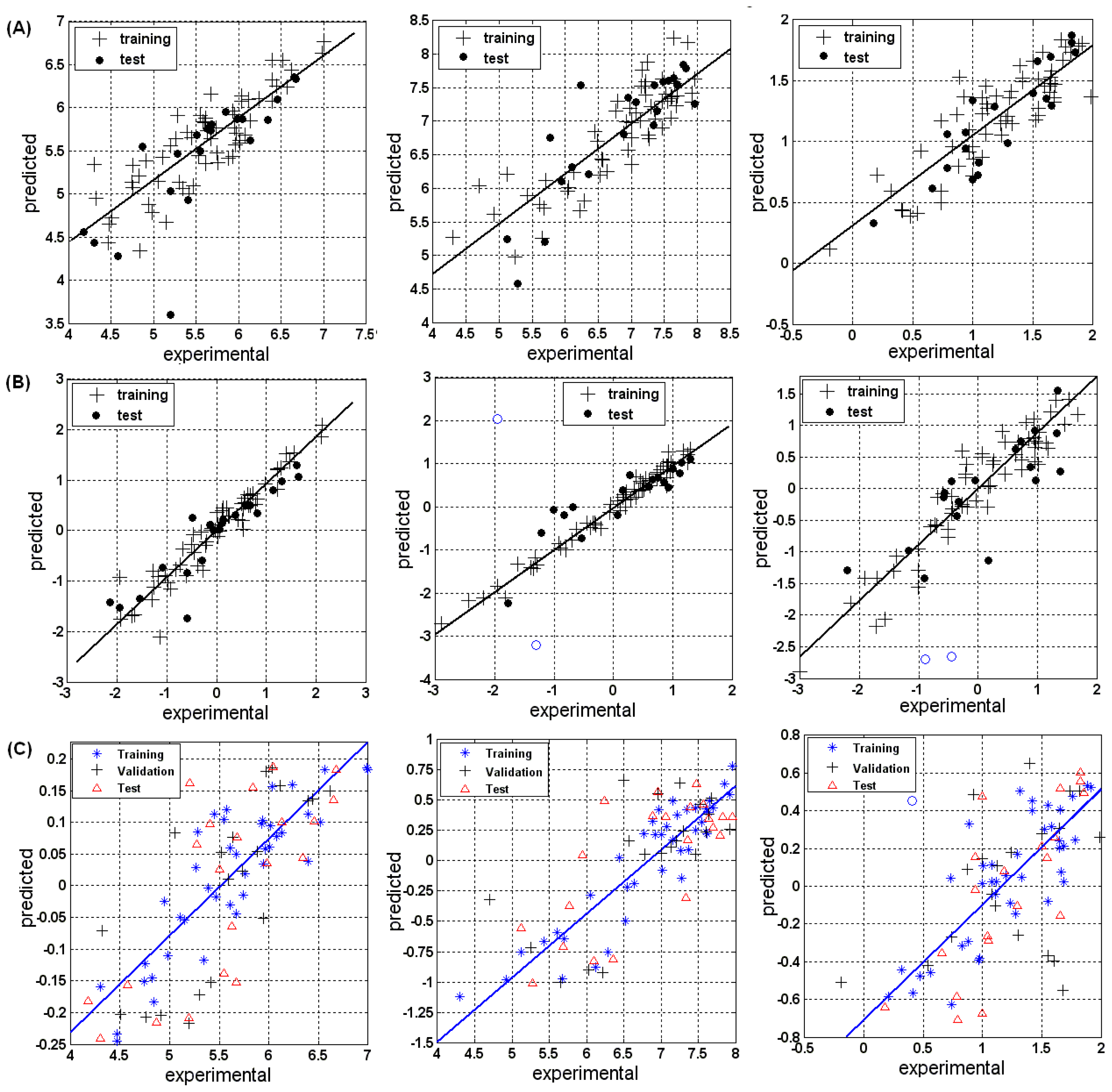
| Data set | A* | B | Rtraining | Rvalidation | Rtest | SSEtraining | SSEvalidation | SSEtest |
|---|---|---|---|---|---|---|---|---|
| alpha | 5 | 5 | 0.87 | 0.76 | 0.73 | 0.19 | 0.09 | 0.10 |
| beta | 5 | 11 | 0.91 | 0.70 | 0.74 | 0.29 | 0.14 | 0.15 |
| Selectivity | 5 | 14 | 0.81 | 0.65 | 0.77 | 0.009 | 0.005 | 0.005 |
| Crystal | AVG_RMSD | SD_RMSD | MAX_RMSD/NO. of pose | MIN_RMSD/NO. of pose |
|---|---|---|---|---|
| 1X7R | 0.66 | 0.18 | 0.94/7th* | 0.46/10th |
| 1X7E | 0.32 | 0.03 | 0.36/9th, 10th | 0.27/5th |
| 1QKM | 0.39 | 0.06 | 0.47/1th, 3th | 0.32/8th |
| 1X78 | 0.53 | 0.32 | 1.04/5th,7th | 0.14/1th |
| 1YY4 | 0.63 | 0.30 | 1.01/7th | 0.14/6th |
| 1YYE | 0.77 | 0.54 | 1.81/7th | 0.34/1th |
© 2010 by the authors; licensee Molecular Diversity Preservation International, Basel, Switzerland. This article is an open-access article distributed under the terms and conditions of the Creative Commons Attribution license (http://creativecommons.org/licenses/by/3.0/).
Share and Cite
Wang, Z.; Li, Y.; Ai, C.; Wang, Y. In Silico Prediction of Estrogen Receptor Subtype Binding Affinity and Selectivity Using Statistical Methods and Molecular Docking with 2-Arylnaphthalenes and 2-Arylquinolines. Int. J. Mol. Sci. 2010, 11, 3434-3458. https://doi.org/10.3390/ijms11093434
Wang Z, Li Y, Ai C, Wang Y. In Silico Prediction of Estrogen Receptor Subtype Binding Affinity and Selectivity Using Statistical Methods and Molecular Docking with 2-Arylnaphthalenes and 2-Arylquinolines. International Journal of Molecular Sciences. 2010; 11(9):3434-3458. https://doi.org/10.3390/ijms11093434
Chicago/Turabian StyleWang, Zhizhong, Yan Li, Chunzhi Ai, and Yonghua Wang. 2010. "In Silico Prediction of Estrogen Receptor Subtype Binding Affinity and Selectivity Using Statistical Methods and Molecular Docking with 2-Arylnaphthalenes and 2-Arylquinolines" International Journal of Molecular Sciences 11, no. 9: 3434-3458. https://doi.org/10.3390/ijms11093434
APA StyleWang, Z., Li, Y., Ai, C., & Wang, Y. (2010). In Silico Prediction of Estrogen Receptor Subtype Binding Affinity and Selectivity Using Statistical Methods and Molecular Docking with 2-Arylnaphthalenes and 2-Arylquinolines. International Journal of Molecular Sciences, 11(9), 3434-3458. https://doi.org/10.3390/ijms11093434