Recent Advances in Fragment-Based QSAR and Multi-Dimensional QSAR Methods

Abstract
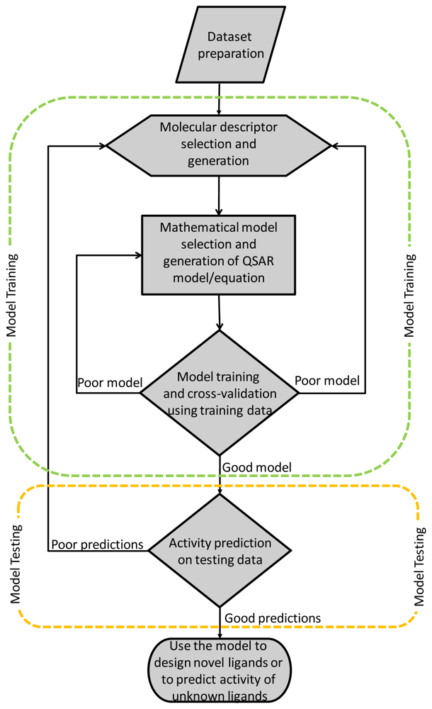
:1. Introduction
2. Fragment-Based 2D-QSAR Methods
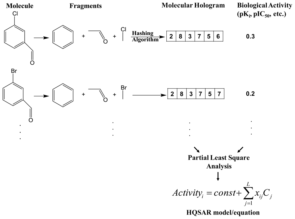
2.1. Hologram-QSAR (HQSAR)
2.2. Fragment-Based QSAR (FB-QSAR)
2.3. Fragment-Similarity Based QSAR (FS-QSAR)
2.4. Top Priority Fragment QSAR
2.5. Other Fragment-Related QSAR Studies
3. 3D-QSAR
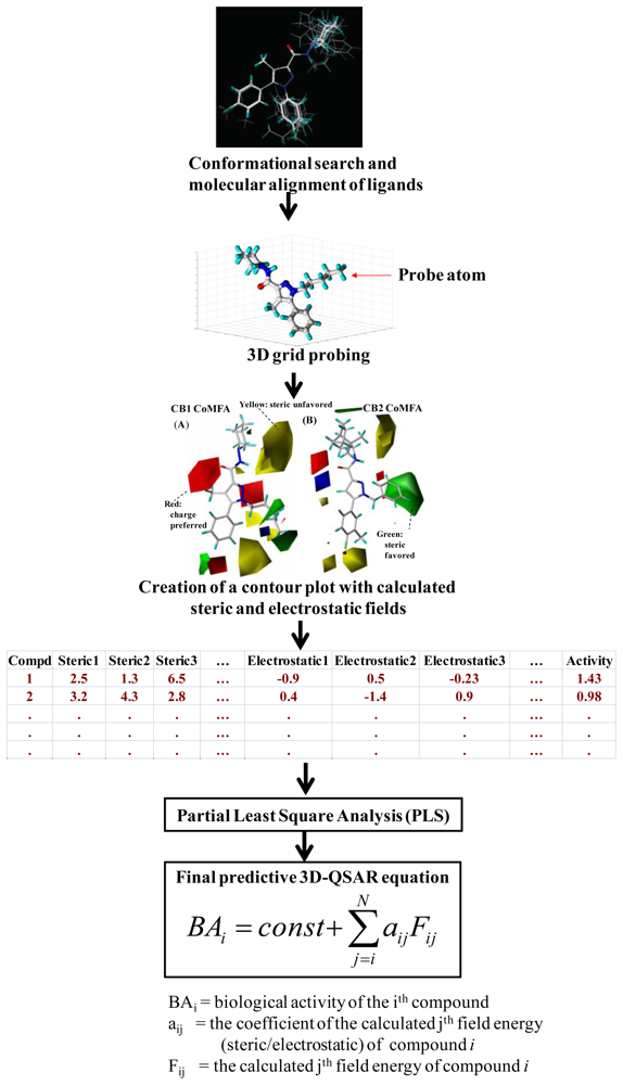
3.1. Comparative Molecular Field Analysis (CoMFA) and Comparative Molecular Similarity Indices Analysis (CoMSIA)
3.2. Topomer CoMFA
3.3. Self-Organizing Molecular Field Analysis (SOMFA)
3.4. Alignment-Free 3D-QSAR Methods
3.4.1. Autocorrelation of Molecular Surfaces Properties (AMSP)
3.4.2. Comparative Molecular Moment Analysis (CoMMA)
3.4.3. Weighted Holistic Invariant Molecular (WHIM) Descriptor-Based QSAR
3.4.4. Grid-Independent Descriptors (GRIND)-Based QSAR
3.5. Multi-Dimensional (nD) QSAR Methods
4. Comparison of 2D or Fragment-Based QSAR versus 3D or nD-QSAR Methods
5. Conclusion
Acknowledgement
References
- Esposito, EX; Hopfinger, AJ; Madura, JD. Methods for applying the quantitative structure-activity relationship paradigm. Methods Mol. Biol 2004, 275, 131–213. [Google Scholar]
- Bradbury, SP. Quantitative structure-activity relationships and ecological risk assessment: an overview of predictive aquatic toxicology research. Toxicol. Lett 1995, 79, 229–237. [Google Scholar]
- Hansch, C; Leo, A. Exploring QSAR—Fundamentals and Applications in Chemistry and Biology; American Chemical Society: Washington, DC., USA, 1995. [Google Scholar]
- Hansch, C; Telzer, BR; Zhang, L. Comparative QSAR in toxicology: Examples from teratology and cancer chemotherapy of aniline mustards. Crit. Rev. Toxicol 1995, 25, 67–89. [Google Scholar]
- Perkins, R; Fang, H; Tong, W; Welsh, W. Quantitative structure-activity relationship methods: perspectives on drug discovery and toxicology. Environ. Toxicol. Chem 2003, 22, 1666–1679. [Google Scholar]
- Chen, J-Z; Han, X-W; Liu, Q; Makriyannis, A; Wang, J; Xie, X-Q. 3D-QSAR studies of arylpyrazole antagonists of cannabinoid receptor subtypes CB1 and CB2. A combined NMR and CoMFA approach. J. Med. Chem 2006, 49, 625–636. [Google Scholar]
- Salum, L; Andricopulo, A. Fragment-based QSAR: Perspectives in drug design. Mol. Divers 2009, 13, 277–285. [Google Scholar]
- Free, SJ; Wilson, J. A mathematical contribution to structure-activity studies. J. Med. Chem 1964, 7, 395–399. [Google Scholar]
- Hansch, CJ; Fujita, T. ρ−σ−π Analysis. A method for the correlation of biological activity and chemical structure. J. Am. Chem. Soc 1964, 86, 1616–1626. [Google Scholar]
- SYBYL8.0. In Discovery Software for Computational Chemistry and Molecular Modeling; Tripos: St. Louis, MO, USA, 2008.
- Lowis, D. HQSAR: A New, Highly Predictive QSAR Technique, Tripos Technique Notes; Tripos: St. Louis, MO, USA, 1997. [Google Scholar]
- Castilho, MS; Postigo, MP; de Paula, CBV; Montanari, CA; Oliva, G; Andricopulo, AD. Two- and three-dimensional quantitative structure-activity relationships for a series of purine nucleoside phosphorylase inhibitors. Bioorg. Med. Chem 2006, 14, 516–527. [Google Scholar]
- Salum, LB; Polikarpov, I; Andricopulo, AD. Structural and chemical basis for enhanced affinity and potency for a large series of estrogen receptor ligands: 2D and 3D QSAR studies. J. Mol. Graph. Model 2007, 26, 434–442. [Google Scholar]
- Honorio, KM; Garratt, RC; Andricopulo, AD. Hologram quantitative structure-activity relationships for a series of farnesoid X receptor activators. Bioorg. Med. Chem. Lett 2005, 15, 3119–3125. [Google Scholar]
- Castilho, MS; Guido, RVC; Andricopulo, AD. 2D Quantitative structure-activity relationship studies on a series of cholesteryl ester transfer protein inhibitors. Bioorg. Med. Chem 2007, 15, 6242–6252. [Google Scholar]
- Lo Piparo, E; Koehler, K; Chana, A; Benfenati, E. Virtual Screening for aryl hydrocarbon receptor binding prediction. J. Med. Chem 2006, 49, 5702–5709. [Google Scholar]
- Tropsha, A; Golbraikh, A. Predictive QSAR modeling workflow, model applicability domains, and virtual screening. Curr. Pharm. Design 2007, 13, 3494–3504. [Google Scholar]
- Prakash, O; Ghosh, I. Developing an antituberculosis compounds database and data mining in the search of a motif responsible for the activity of a diverse class of antituberculosis agents. J. Chem. Inf. Model 2005, 46, 17–23. [Google Scholar]
- Du, Q-S; Huang, R-B; Wei, YT; Pang, Z-W; Du, L-Q; Chou, K-C. Fragment-based quantitative structure-activity relationship (FB-QSAR) for fragment-based drug design. J. Comput. Chem 2009, 30, 295–304. [Google Scholar]
- Myint, KZ; Ma, C; Wang, L; Xie, XQ. The Fragment-similarity-based QSAR (FS-QSAR): A Novel 2D-QSAR method to predict biological activities of triaryl Bis-sulfone and COX2 analogs. 2010. submitted. [Google Scholar]
- Burden, F. Molecular identification number for substructure searches. J. Chem. Inf. Comput. Sci 1989, 29, 225–227. [Google Scholar]
- Xie, XQ; Chen, J. Data-mining a small molecule drug screening representative subset from NIH PubChem database. J. Chem. Inf. Model 2008, 48, 465–475. [Google Scholar]
- Casalegno, M; Sello, G. Benfenati E: Top-Priority Fragment QSAR Approach in Predicting Pesticide Aquatic Toxicity. Chem. Res. Toxicol 2006, 19, 1533–1539. [Google Scholar]
- Zhokhova, N; Baskin, I; Palyulin, V; Zefirov, A; Zefirov, N. Fragmental descriptors with labeled atoms and their application in QSAR/QSPR studies. Doklady Chem 2007, 417, 282–284. [Google Scholar]
- Ford, MG. Euroqsar 2002 Designing Drugs and Crop Protectants: Processes, Problems, and Solutions; Blackwell: Melbourne, Australia, 2003. [Google Scholar]
- Andrade, C; Salum, LB; Castilho, M; Pasqualoto, K; Ferreira, E; Andricopulo, A. Fragment-based and classical quantitative structure–activity relationships for a series of hydrazides as antituberculosis agents. Mol. Divers 2008, 12, 47–59. [Google Scholar]
- Dragon, v5.4; Talete_Srl: Milan, Italy, 2008.
- Oliveira, DBD; Gaudio, AC. BuildQSAR: A new computer program for QSAR analysis. Quant. Struct.-Act. Relation 2000, 19, 599–601. [Google Scholar]
- Pirouette Multivariate Data Analysis for IBM PC Systems; Infometrix: Seattle, WA, USA, 2001.
- Tsygankova, I; Zhenodarova, S. Quantitative structure-activity relationship for barbituric acid derivatives: Potential of the fragment approach. Russ. J. Gene. Chem 2007, 77, 940–928. [Google Scholar]
- Cramer, R; Patterson, D; Bunce, J. Comparative molecular field analysis (CoMFA). 1. Effect of shape on binding of steroids to carrier proteins. J. Am. Chem. Soc 1988, 110, 5959–5967. [Google Scholar]
- Klebe, G; Abraham, U; Mietzner, T. Molecular similarity indices in a comparative analysis (CoMSIA) of drug molecules to correlate and predict their biological activity. J. Med. Chem 1994, 37, 4130–4146. [Google Scholar]
- Dudek, AZ; Arodz, O; Galvez, J. Computational methods in developing quantitative structure-activity relationships (QSAR): A review. Comb. Chem. High T. Scr 2006, 9, 213–228. [Google Scholar]
- Cramer, RD; Cruz, P; Stahl, G; Curtiss, WC; Campbell, B; Masek, BB; Soltanshahi, F. Virtual screening for r-groups, including predicted pIC50 contributions, within large structural databases, using topomer CoMFA. J. Chem. Inf. Model 2008, 48, 2180–2195. [Google Scholar]
- Avram, S; Milac, AL; Flonta, ML. Computer-aided drug design for typical and atypical antipsychotic drugs: A review of application of QSAR and combinatorial chemistry methods - tools for new antipsychotics design. Curr. Comput.-Aided Drug Design 2005, 1, 347–364. [Google Scholar]
- Patcharawee, N; Nahoum, GA; Blair, FJ; Simon, PM; Jiraporn, U. 3D-QSAR studies on chromone derivatives as HIV-1 protease inhibitors: Application of molecular field analysis. Arch. Pharm 2008, 341, 357–364. [Google Scholar]
- Labrie, P; Maddaford, SP; Fortin, S; Rakhit, S; Kotra, LP; Gaudreault, RC. A comparative molecular field analysis (CoMFA) and comparative molecular similarity indices analysis (CoMSIA) of anthranilamide derivatives that are multidrug resistance modulators. J. Med. Chem 2006, 49, 7646–7660. [Google Scholar]
- Jeong, JA; Cho, H; Jung, SY; Kang, HB; Park, JY; Kim, J; Choo, DJ; Lee, JY. 3D QSAR studies on 3,4-dihydroquinazolines as T-type calcium channel blocker by comparative molecular similarity indices analysis (CoMSIA). Bioorg. Med. Chem. Lett 2010, 20, 38–41. [Google Scholar]
- Dayan, FE; Singh, N; McCurdy, CR; Godfrey, CA; Larsen, L; Weavers, RT; van Klink, JW. Perry NB: β-triketone inhibitors of plant p-hydroxyphenylpyruvate dioxygenase: Modeling and comparative molecular field analysis of their interactions. J. Agric. Food Chem 2009, 57, 5194–5200. [Google Scholar]
- Cramer, RD. Topomer CoMFA: A design methodology for rapid lead optimization. J. Med. Chem 2003, 46, 374–388. [Google Scholar]
- Robinson, DD; Winn, PJ; Lyne, PD; Richards, WG. Self-organizing molecular field analysis: A tool for structure-activity studies. J. Med. Chem 1999, 42, 573–583. [Google Scholar]
- Bravi, G; Gancia, E; Mascagni, P; Pegna, M; Todeschini, R; Zaliani, A. MS-WHIM, new 3D theoretical descriptors derived from molecular surface properties: A comparative 3D QSAR study in a series of steroids. J. Comput.-Aided Mol. Design 1997, 11, 79–92. [Google Scholar]
- Wagener, M; Sadowski, J; Gasteiger, J. Autocorrelation of molecular surface properties for modeling corticosteroid binding globulin and cytosolic ah receptor activity by neural networks. J. Am. Chem. Soc 1995, 117, 7769–7775. [Google Scholar]
- Silverman, BD; Platt, DE. Comparative molecular moment analysis (CoMMA): 3D-QSAR without molecular superposition. J. Med. Chem 1996, 39, 2129–2140. [Google Scholar]
- Todeschini, R; Gramatica, P. Kubinyi, H, Folkers, G, Martin, YC, Eds.; New 3D molecular descriptors: the WHIM theory and QSAR applications. In 3D QSAR in Drug Design; Kluwer Academic Publishers/Escom: Dordrecht, The Netherlands, 1998; Volume 2, pp. 355–380. [Google Scholar]
- Todeschini, R; Lasagni, M. Marengo E: New molecular descriptors for 2D and 3D structures. J. Chemometrics 1994, 8, 263–272. [Google Scholar]
- Pastor, M; Cruciani, G; McLay, I; Pickett, S; Clementi, S. GRid-INdependent descriptors (GRIND): A novel class of alignment-independent three-dimensional molecular descriptors. J. Med. Chem 2000, 43, 3233–3243. [Google Scholar]
- Connolly, M. Analytical molecular surface calculation. J. Appl. Crystallogr 1983, 16, 548–558. [Google Scholar]
- Pastor, M; Cruciani, G; Watson, KA. A strategy for the incorporation of water molecules present in a ligand binding site into a three-dimensional quantitative structure-activity relationship analysis. J. Med. Chem 1997, 40, 4089–4102. [Google Scholar]
- ALMOND. Molecular Discovery Ltd: Perugia, Italy. Available at: http://www.moldiscovery.com/soft_almond.php (accessed on 25 September 2010).
- Hopfinger, AJ; Wang, S; Tokarski, JS; Jin, B; Albuquerque, M; Madhav, PJ; Duraiswami, C. Construction of 3D-QSAR models using the 4D-QSAR analysis formalism. J. Am. Chem. Soc 1997, 119, 10509–10524. [Google Scholar]
- Scheiber, J; Enzensperger, C; Lehmann, J; Stiefl, N; Baumann, K. Aki-Sener, E, Yalcin, I, Eds.; Alignment-free 4D-QSAR: Applying the XMAP technique in prospective analyses. In QSAR & Molecular Modeling in Rational Design of Bioactive Molecules; CADDD Society: Ankara, Turkey, 2006. [Google Scholar]
- Fischer, PM. Computational chemistry approaches to drug discovery in signal transduction. Biotechnol. J 2008, 3, 452–470. [Google Scholar]
- Vedani, A; Dobler, M. 5D-QSAR: The key for simulating induced fit? J. Med. Chem 2002, 45, 2139–2149. [Google Scholar]
- Vedani, A; Dobler, M; Lill, MA. Combining protein modeling and 6D-QSAR. Simulating the binding of structurally diverse ligands to the estrogen receptor. J. Med. Chem 2005, 48, 3700–3703. [Google Scholar]
- Vedani, A; Dobler, M; Zbinden, P. Quasi-atomistic receptor surface models: A bridge between 3-D QSAR and receptor modeling. J. Am. Chem. Soc 1998, 120, 4471–4477. [Google Scholar]
- Biograf. VirtualToxLab: Basel, Switzerland, 2009. Available at: http://www.biograf.ch/downloads/VirtualToxLab.pdf (accessed on 25 September 2010).
- Hillebrecht, A; Klebe, G. Use of 3D QSAR models for database screening: A feasibility study. J. Chem. Inf. Model 2008, 48, 384–396. [Google Scholar]
- Matter, H; Potter, T. Comparing 3D pharmacophore triplets and 2D fingerprints for selecting diverse compound subsets. J. Chem. Inf. Comput. Sci 1999, 39, 1211–1225. [Google Scholar]
- Khedkar, V; Ambre, P; Verma, J; Shaikh, M; Pissurlenkar, R; Coutinho, E. Molecular docking and 3D-QSAR studies of HIV-1 protease inhibitors. J. Mol. Model 2010, 16, 1251–1268. [Google Scholar]
- Li, Q; J⊘rgensen, FS; Oprea, T; Brunak, S; Taboureau, O. hERG classification model based on a combination of support vector machine method and GRIND descriptors. Mol. Pharm 2008, 5, 117–127. [Google Scholar]
- Romeiro, N; Albuquerque, M; Alencastro, R; Ravi, M; Hopfinger, A. Construction of 4D-QSAR models for use in the design of novel p38-MAPK inhibitors. J. Comput.-Aided Mol. Design 2005, 19, 385–400. [Google Scholar]


| Method | nD | Dataset | Statistical model | Performance | Reference/Website |
|---|---|---|---|---|---|
| HQSAR | 2D | 21 Steroids | PLS | q2 = 0.71; r2 = 0.85 [11] | [11] http://www.tripos.com |
| FB-QSAR | 2D | 48 NA analogs | IDLS | r = 0.95 (r2 = 0.91) [19] | [19] |
| FS-QSAR | 2D | 85 bis-sulfone analogs; 83 COX2 analogs | MLR | r2 = 0.68; r2 = 0.62 [20] | [20] |
| TPF-QSAR | 2D | 282 pesticides | PM-based prediction | r2 = 0.75 [23] | [23] |
| CoMFA | 3D | 21 Steroids 54 HIV-1PR inhibitors | PLS | q2 = 0.75; r2 = 0.96 [11] q2 = 0.68; r2 = 0.69 [60] | [31] http://www.tripos.com [60] |
| CoMSIA | 3D | Thermolysin inhibitors 54 HIV-1PR inhibitors | PLS | q2 = [0.59, 0.64] [32] q2 = 0.65; r2 = 0.73 [60] | [61,62] http://www.tripos.com [60] |
| Topomer CoMFA | 3D | 15 datasets from literature | PLS | average q2 = 0.636 [40] | [40] http://www.tripos.com |
| SOMFA | 3D | 31 steroids; 35 sulfonamides | MLR | r2 = 0.58; r2 = 0.53 [41] | [41] |
| AMSP | 3D | 31 steroids | MNN | q2 = 0.63; r2 = 0.67 [43] | [43] |
| CoMMA | 3D | 31 steroids | PLS | q2 = [0.41, 0.82] [44] | [44] |
| WHIM | 3D | 31 steroids | PCA | SDEP = 1.750 [42] | [45] http://www.vcclab.org/lab/indexhlp/whimdes.html |
| MS-WHIM | 3D | 31 steroids | PCA | SDEP = 0.742 [42] | [42] |
| GRIND | 3D | 31 steroids 175 hERG inhibitors | PLS; PCA PLS; SVM | q2 = 0.64; SDEP = 0.26 [47] q2 = 0.41; r2 = 0.57; SDEP = 0.72 [63] | [47] http://www.moldiscovery.com/soft_grid.php [63] |
| 4D-QSAR | 4D | 20 DHFR inhibitors; 42 PGF2a analogs; 40 2-substituted dipyridodiazepione inhibitors 33 p38-MAPK inhibitors | PLS GL-PLS | r2 = [0.90, 0.95]; r2 = [0.73, 0.86]; r2 = [0.67, 0.76] [51] q2 = [0.67, 0.85] [64] | [51] http://www.seascapelearning.com/4DsgiSW/ [64] |
| 5D-QSAR | 5D | 65 NK-1 antagonists; 131 Ah ligands | MLR | r2 = 0.84; r2 = 0.83 [54] | [54] http://www.biograf.ch |
| 6D-QSAR | 6D | 106 estrogen receptor ligands | MLR | q2 = 0.90; r2 = 0.89 [55] | [55] http://www.biograf.ch |
| HQSAR = Hologram QSAR FB-QSAR = Fragment-based QSAR FS-QSAR = fragment-similarity-based QSAR TPF-QSAR = Top priority fragment QSAR CoMFA = Comparative molecular field analysis CoMSIA = Comparative molecular similarity indices analysis SOMFA = Self-organizing molecular field analysis AMSP = Autocorrelation of molecular surface properties CoMMA = Comparative molecular moment analysis WHIM = Weighted holistic invariant molcular QSAR MS-WHIM = Molecular surface WHIM GRIND = Grid independent descriptor | PLS = Partial least square IDLS = Iterative double least square PM = Priority matrix MNN = Multilayer neural networks MLR = Multiple linear regression PCA = Principal component analysis | q2 = cross-validated r2 SDEP = standard deviation of errors of prediction | |||
© 2010 by the authors; licensee Molecular Diversity Preservation International, Basel, Switzerland. This article is an open-access article distributed under the terms and conditions of the Creative Commons Attribution license (http://creativecommons.org/licenses/by/3.0/).
Share and Cite
Myint, K.Z.; Xie, X.-Q. Recent Advances in Fragment-Based QSAR and Multi-Dimensional QSAR Methods. Int. J. Mol. Sci. 2010, 11, 3846-3866. https://doi.org/10.3390/ijms11103846
Myint KZ, Xie X-Q. Recent Advances in Fragment-Based QSAR and Multi-Dimensional QSAR Methods. International Journal of Molecular Sciences. 2010; 11(10):3846-3866. https://doi.org/10.3390/ijms11103846
Chicago/Turabian StyleMyint, Kyaw Zeyar, and Xiang-Qun Xie. 2010. "Recent Advances in Fragment-Based QSAR and Multi-Dimensional QSAR Methods" International Journal of Molecular Sciences 11, no. 10: 3846-3866. https://doi.org/10.3390/ijms11103846
APA StyleMyint, K. Z., & Xie, X.-Q. (2010). Recent Advances in Fragment-Based QSAR and Multi-Dimensional QSAR Methods. International Journal of Molecular Sciences, 11(10), 3846-3866. https://doi.org/10.3390/ijms11103846