Impersonality of the Connectivity Index and Recomposition of Topological Indices According to Different Properties

Abstract

The connectivity index χ can be regarded as the sum of bond contributions. In this article, boiling point (bp)-oriented contributions for each kind of bond are obtained by decomposing the connectivity indices into ten connectivity character bases and then doing a linear regression between bps and the bases. From the comparison of bp-oriented contributions with the contributions assigned by χ, it can be found that they are very similar in percentage, i.e. the relative importance of each particular kind of bond is nearly the same in the two forms of combinations (one is obtained from the regression with boiling point, and the other is decided by the constructor of the χ index). This coincidence shows an impersonality of χ on bond weighting and may provide us another interpretation of the efficiency of the connectivity index on many quantitative structure– activity/property relationship (QSAR or QSPR) results. However, we also found that χ’s weighting formula may not be appropriate for some other properties. In fact, there is no universal weighting formula appropriate for all properties/activities. Recomposition of some topological indices by adjusting the weights upon character bases according to different properties/activities is suggested. This idea of recomposition is applied to the first Zagreb group index M₁ and a large improvement has been achieved.

Introduction

Since the first topological index – the W index [1] was developed and found useful in finding correlations between property and chemical structures, more and more chemists came to know its merits and tried to propose novel topological indices to construct better QSAR/QSPR models. They compiled numerical characterizations of the chemical structure of molecules by means of various graph matrices, distances, walks and paths counts. Then, a large variety of mathematical operations were applied to the numerical molecular characters giving novel topological indices (TIs). Different operators on one character can even produce several topological indices, and in this way, more than 400 TIs have been proposed. They have contributed greatly to the widespread use of QSAR/QSPR models, but this indiscriminate proliferation of topological indices has produced some criticisms from skeptics of the use of this approach in chemistry: “This disorientation in the search of such molecular descriptors often produces no good correlation with any property, and looks very convoluted in their definition” [2]. As a result, among hundreds of existing topological indices, only a small number of them are widely used by the QSAR/QSPR researchers.

In 1975, Randić proposed the connectivity index χ with the initial name “branching index” [3]. Within a short time Kier and Hall had recognized its merits, not only its description ability for molecular branching, but also that the correlation ability of χ was also quite good for many physical and biochemical properties. They demonstrated its use for a wide range of compounds and properties [4,5]. Until now, the connectivity index is still most widely used. Some researchers have studied the reason why it is so popular and drawn some conclusions on its success. For instance, Randić has attributed it to its greater weighting of terminal CC bonds and lesser weighting of internal CC bonds [6]. Working over several famous topological indices by partitioning them into bond additive terms it was then found that better regressions resulted when terminal CC bonds gave more contribution and internal bonds gave less. This conclusion can interpret, to some extent, the correlation between some properties and molecular structure. However, it seems more like a qualitative interpretation than a quantitative one. When faced with various available weighting formulae like {(mn)^-1, (mn)^-½, (mn)^-⅓,...} for bond (m, n), which should be the best, why (mn)^-½? Using connectivity character bases, a novel interpretation is proposed for the success of the connectivity index χ with its impersonality on the bond weighting formula. In 1991, the variable connectivity index was proposed by Randić [7] as an alternative approach to Kier and Hall’s valence connectivity index [8] for characterization of heterosystems in QSPR studies. The difference between the variable connectivity index and the valence connectivity index is that the former uses optimized vertex-weights while the latter uses fixed vertex-weights. The main advantage of such variable connectivity index lies in the fact that different molecular properties require distinct optimal parameters. There is no universal valence connectivity index that would apply to all properties of the heteroatomic structures, but the variable connectivity index can adjust to the individual requirements of different molecules and molecular properties. For the same reason, more general variable topological indices are considered in our present work. Using topological character bases, some TIs can be recomposed by adjusting the weights upon the character bases according to different properties/activities. This recomposition makes it possible that the character bases can give full scope to their potential abilities on property description. As an example, the first Zagreb group index M₁ [9] is recomposed according to different properties and then the optimized M₁ index will show large improvement in building regression models.

The connectivity character base set

The connectivity index was first proposed to parallel relative magnitudes of boiling points in smaller alkanes [3]. After 27 years, this index is still most widely used among all TIs [10] with its well-known definition:

$$\chi ={\displaystyle \sum _{alledges}{(v_i{v}_j)}^{-1/2}}$$

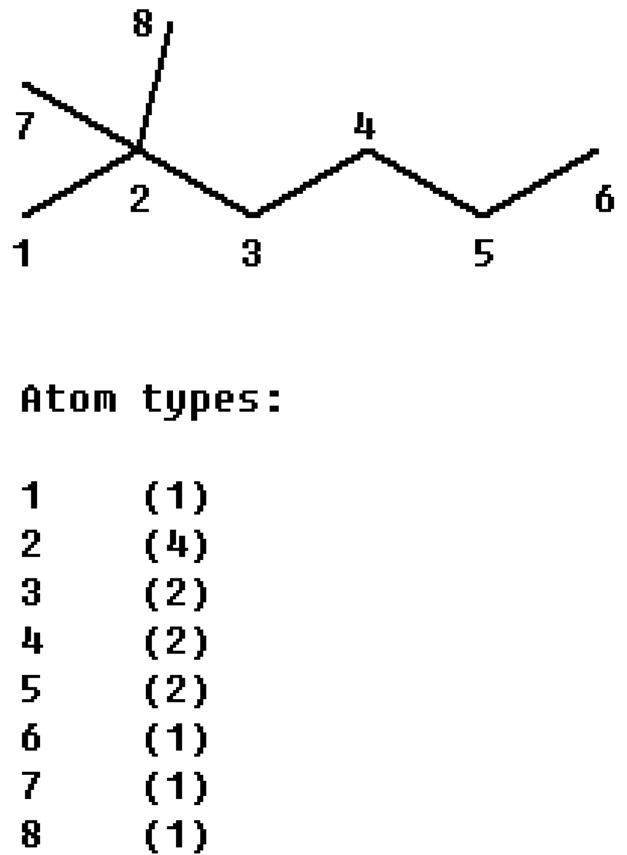
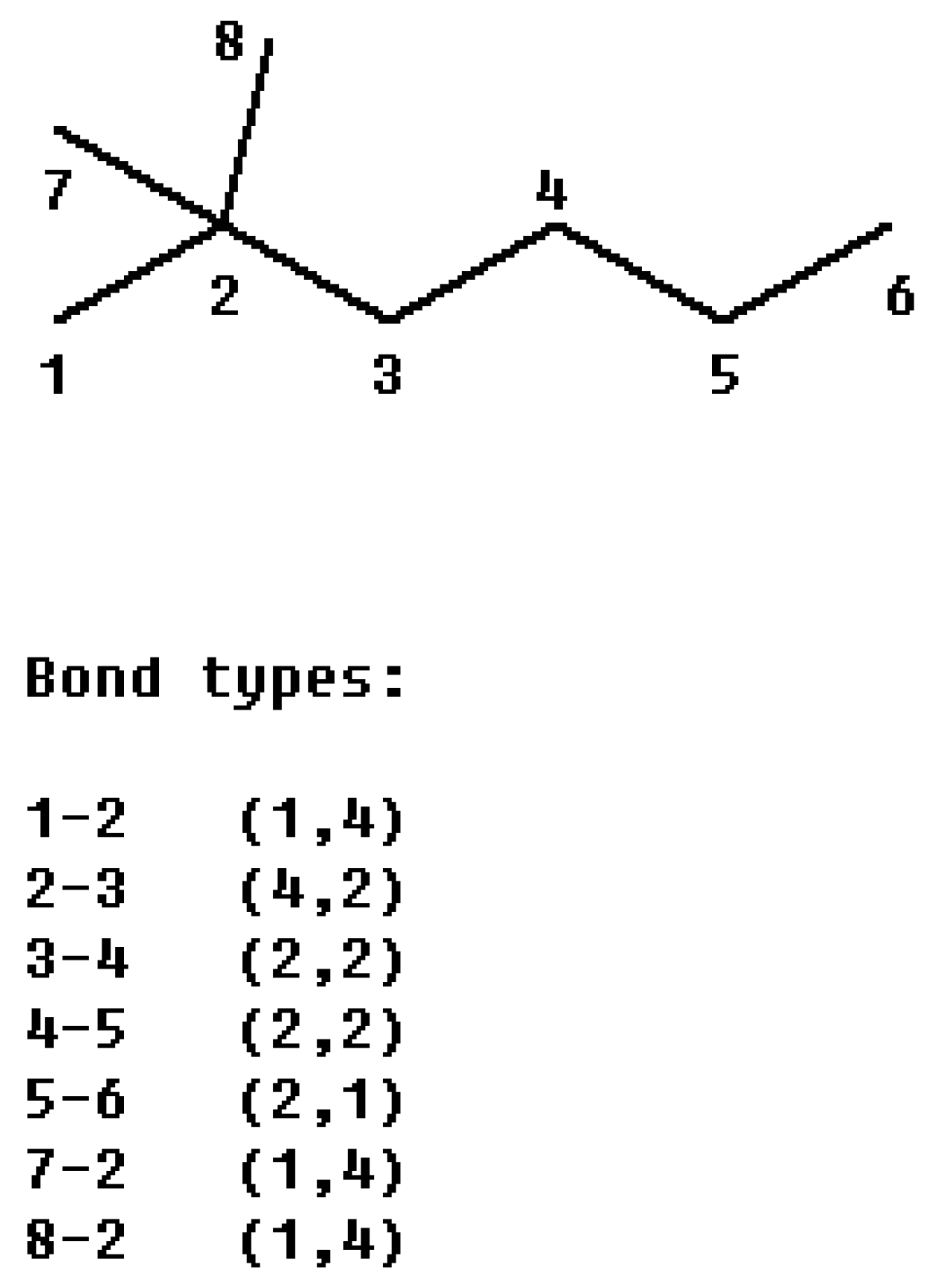
where $(v_i,v_j)$ denotes one pair of vertex degrees on both sides of an edge (bond) and (i, j) the orders of the two atoms on the bond. For example, from the 2, 2-dimethylhexane (Figure 1) we obtain:

$$\begin{array}{ll}\hfill \chi & ={(1\times 4)}^{-1/2}+{(1\times 4)}^{-1/2}+{(1\times 4)}^{-1/2}+{(2\times 4)}^{-1/2}+{(2\times 2)}^{-1/2}+{(2\times 2)}^{-1/2}+{(1\times 2)}^{-1/2}\hfill \\ \hfill & =\mathrm{3.5607.}\hfill \end{array}$$

Figure 1. The partitioning of the connectivity index of 2, 2-dimethylhexane into bond contributions.

Figure 1. The partitioning of the connectivity index of 2, 2-dimethylhexane into bond contributions.

Since the χ index is a bond additive mathematical invariant, the process of its calculation can be divided into two steps: first classify the bond into the (m, n) bond type according to the valences of two atoms forming the bond, and then the value of χ is given by summing the contributions of the form (mn)^-½ over all the bonds of hydrogen-suppressed molecular graph. For saturated hydrocarbons, there are 10 kinds of CC bonds: {(1, 1), (1, 2), (1,3), (1, 4), (2, 2), (2, 3), (2, 4), (3, 3), (3, 4), (4, 4)}. Accordingly, we define the connectivity character base set $\{{\chi }_{11}$, ${\chi }_{12}$, ${\chi }_{13}$, ${\chi }_{14}$, ${\chi }_{22}$, ${\chi }_{23}$, ${\chi }_{24}$, ${\chi }_{33}$, ${\chi }_{34}$, ${\chi }_{44}\}$, where base ${\chi }_{mn}$ is the frequency of occurrence of each kind of edge in the molecular graph. What the χ index does is assign a contribution (mn)^-½ to the (m, n) bond and sum all the contributions. It should be noticed that same bonds were appointed to the same contribution. Another way of calculating the contribution of all (m, n) bonds is to multiply each assigned weight (mn)^-½ by base ${\chi }_{mn}$, the count of (m, n) bonds. Using the character bases, the definition of the connectivity index can be written as:

$$\chi ={\displaystyle \sum _{allbases}{(mn)}^{-1/2}{\chi }_{mn}}$$

The connectivity character bases for 2,2-dimethylhexane are { ${\chi }_{11}$-0, ${\chi }_{12}$-1, ${\chi }_{13}$-0, ${\chi }_{14}$-3, ${\chi }_{22}$-2, ${\chi }_{23}$-0, ${\chi }_{24}$-1, ${\chi }_{33}$-0, ${\chi }_{34}$-0, ${\chi }_{44}$-0}, according to this definition, the χ index can be calculated as:

$$\begin{array}{ll}\hfill \chi & ={(1\times 2)}^{-1/2}\times 1+{(1\times 4)}^{-1/2}\times 3+{(2\times 2)}^{-1/2}\times 2+{(2\times 4)}^{-1/2}\times 1\hfill \\ \hfill & =\mathrm{3.5607.}\hfill \end{array}$$

From this definition, the connectivity index χ can be viewed as a linear combination of the ten character bases while the combination weight assigned to each kind of base is (mn)^-½. To find out some impersonality of the assigned weight (mn)^-½, in this article, 530 boiling points (bps) of all the saturated hydrocarbons (from acyclic to polycyclic) with carbon numbers from 2 to 10 [11] are collected for the calculation of the bp-oriented weights. Numerical values of the bp-oriented weights were calculated by least squares, i.e. contributions for different bonds are decided by taking the bases as variables, bps as response and make linear regression between them. Because the regression coefficients in linear model will exhibit a relative importance of variables to the response, they can be regarded as the bp-oriented weights on the character bases. In the step of pretreatment, we found that base χ₁₁ is non-zero only for ethane, thus to avoid a singularity in the linear regression, ethane is deleted from our data set. Then χ₁₁ can be ignored in the linear model construction. The bp-oriented weights (regression coefficients) obtained from the rest 9 bases and 529 boiling points are listed in Table 1.

It is hard to make a fair comparison just from Table 1 because of different scales of the two sets of weights. To eliminate the influence brought by different scales, percentage of each weight is calculated by dividing the sum. For example, assume the original weights are 2, 4, 6, 8 for base 1, 2 3, 4, the percentage can be obtained by dividing each weight by the sum 2+4+6+8=20, then we get 2/20, 4/20, 6/20, 8/20 as the percentage for base 1, 2, 3, 4, respectively. After normalization, the relative importance of all connectivity character bases to the property--boiling point can be expressed clearly as percentages (Table 2). Plot of the normalized χ weights vs. normalized bp-oriented weights (Reg. Coef.) are given in Figure 2 (a).

Table 1. χ’s weights and regression coefficients.

	χ12	χ13	χ14	χ22	χ23	χ24	χ33	χ34	χ44
χ weights	0.707	0.577	0.500	0.500	0.408	0.354	0.333	0.289	0.250
Reg. Coef.	37.88	31.99	29.54	29.01	22.62	18.10	19.04	14.93	14.12

Table 1. χ’s weights and regression coefficients.

	χ12	χ13	χ14	χ22	χ23	χ24	χ33	χ34	χ44
χ weights	0.707	0.577	0.500	0.500	0.408	0.354	0.333	0.289	0.250
Reg. Coef.	37.88	31.99	29.54	29.01	22.62	18.10	19.04	14.93	14.12

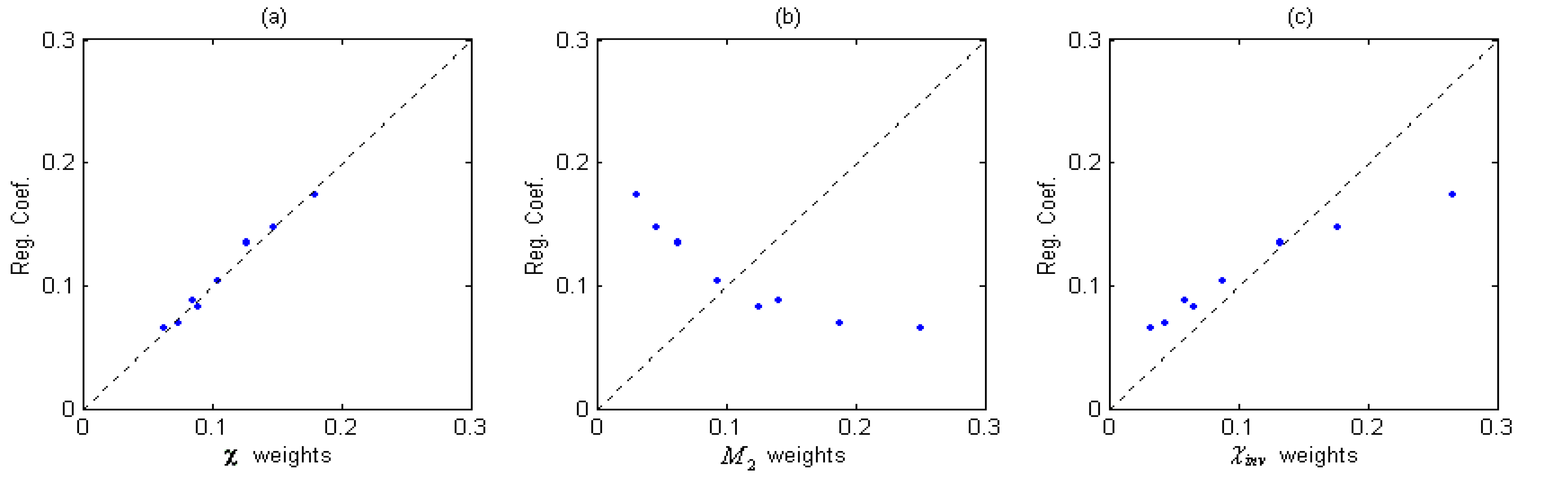
Figure 2. Plot of (a) χ weights vs. Reg. Coef., (b) M₂ weights vs. Reg. Coef. and (c) χ_inv weights vs. Reg. Coef. (Normalized).

Figure 2. Plot of (a) χ weights vs. Reg. Coef., (b) M₂ weights vs. Reg. Coef. and (c) χ_inv weights vs. Reg. Coef. (Normalized).

Table 2. Comparison of regression coefficients (Reg. Coef.) and weights assigned by χ, M₂ and χ_inv (normalized).

	χ12	χ13	χ14	χ22	χ23	χ24	χ33	χ34	χ44
M2 weights	0.031	0.047	0.063	0.063	0.094	0.125	0.141	0.188	0.250
χinv weights	0.266	0.178	0.133	0.133	0.089	0.067	0.059	0.044	0.033
χ weights	0.181	0.147	0.128	0.128	0.104	0.090	0.085	0.074	0.064
Reg. Coef.	0.174	0.147	0.136	0.134	0.104	0.083	0.088	0.069	0.065

Table 2. Comparison of regression coefficients (Reg. Coef.) and weights assigned by χ, M₂ and χ_inv (normalized).

	χ12	χ13	χ14	χ22	χ23	χ24	χ33	χ34	χ44
M2 weights	0.031	0.047	0.063	0.063	0.094	0.125	0.141	0.188	0.250
χinv weights	0.266	0.178	0.133	0.133	0.089	0.067	0.059	0.044	0.033
χ weights	0.181	0.147	0.128	0.128	0.104	0.090	0.085	0.074	0.064
Reg. Coef.	0.174	0.147	0.136	0.134	0.104	0.083	0.088	0.069	0.065

It can be found from Table 2 and Figure 2(a) that the χ weights are very close to the bp-oriented weights which are obtained from the linear regression when the property of boiling point is considered. Thus, weight (mn)^-½ assigned to corresponding bonds seems more property-oriented-like than subjectively decided by its constructor, and this interesting coincidence exhibits the impersonality of the χ’s weights. Here the impersonality of a topological index means that the construction of the index is not only representing the subjective understanding of its proposer but also indicating a close relationship with some property or activities. Then we will try to show that this impersonality of χ’s weighting formula is an important reason for its great success.

Let us investigate on χ and two other topological indices. All of them are constructed on same character bases but very different achievements on property interpretations. One is the second Zagreb group index M₂ [7] that assigns m x n to base χ_mn as:

$$M_2={\displaystyle \sum _{allbases}(mn){\chi }_{mn}}$$

On the other hand, suppose another topological index χ_inv is designed on the same χ character bases as follows:

$${\chi }_{inv}={\displaystyle \sum _{allbases}{(mn)}^{-1}{\chi }_{mn}}$$

Similarly to χ, this index assigns greater weights on terminal CC bonds and lesser weights on internal CC bonds while M₂ does the opposite. Applying these three different weighting formulae on the connectivity character bases we get χ, M₂ and χ_inv. Then, boiling points of the 529 alkanes are used as a particular property giving some regression results. Among the three indices χ is the best one in fitting with this property, with a standard deviation (SD) of 7.6788 and R of 0.9802, then comes χ_inv with SD = 21.7452 and R = 0.8278, the last is M₂ with SD = 34.1617 and R = 0.4724. To find out why the χ’s weighting formula is the most effective one, the weight percentages of the other two indices are also listed in Table 2. Plots of the assigned weights vs. regression coefficients from these two indices are represented in Figure 2 (b) and Figure 2 (c).

It can be seen clearly from Figure 2 that the bond-contributions assigned by M₂ is quite different from the bp-oriented (Reg. Coef.) ones, χ_inv is closer but still has a little deviation, but we can find a perfect coincidence in (a). At the same time, we should notice that the only difference among the three TIs lies in their weighting formulae. That is to say, different combinations on the same connectivity character bases bring large variety of their regression achievements. From the comparison, it seems that the regression progress of such topological indices in QSPR model has a direct proportion to the degree of agreement between the weights on character bases with the regression coefficients.

The recomposition of TIs according to different properties

In previous section we have shown the impersonality of the χ’s weighting formula when boiling point is considered. In this section, six properties have been collected for further investigation, they are: boiling point at normal pressure [11], GC retention index (RI) [12], vapor pressure (VapP) at temperature of 25 ºC [13,14,15], density [16], refraction constant values (Refra) [16,17] and Critical Pressure (CP) [16,18]. Except the values of boiling point and retention index which can be easily found in the references, all the property values used are presented in Table 3. The connectivity index χ, the second Zagreb group index M₂ and the connectivity character bases are used to build relationships with these properties. Results of R values in corresponding linear models are listed in Table 4.

Table 3. Alkanes and their properties.

Alkanes a	VapPa	Density	Refra	CP	Alkanes a	VapPa	Density	Refra	CP
n2	6.63				23mn6	3.54	0.7121	1.4011	25.96
n3	5.979			41.92	34mn6	3.33	0.7192	1.4041
n4	5.36			37.47	3e2mn5	3.56	0.7193	1.404	26.65
2mn3	5.38	0.557		36	234mn5	3.55	0.719	1.4042
c4	5.15				33mn6	3.64	0.71	1.4001
n5	4.835	0.626	1.3577	33.26	224mn5	3.8	0.6919	1.3915	25.34
2mn4	4.94	0.6197		33.37	3e3mn5	3.49
22mn3	5.26			31.57	223mn5	3.63	0.716	1.403	26.94
c5	4.6	0.7457	1.4062	44.43	233mn5	3.55	0.7256	1.4075	27.83
n6	4.46	0.6603	1.3749	29.85	1pc5	3.08	0.7763	1.4266
2mn5	4.46	0.6599	1.3715	29.71	1ipc5	3.33
3mn5	4.4	0.6643	1.3765	30.83	1elmc5	3.41
23mn4	4.51	0.6616	1.375	30.86	1ec6	3.24	0.7879	1.433	30
22mn4	4.6	0.6492	1.3688	30.4	14mc6				29
1mc5	4.28	0.7486	1.4097	37.35	13mc6				29
c6	4.11	0.7785	1.4262	40.22	12mc6				29
n7	3.76	0.6838	1.3877	27.04	11mc6	3.48		1.428
2mn6	3.91	0.6786	1.3849	26.98	c8	2.85
3mn6	3.91	0.6868	1.3886	27.77	n9	2.56	0.7176		22.6
3en5	3.92	0.6982	1.3934		2mn8	2.93
24mn5	4.12	0.6727	1.3815		3mn8	2.91
23mn5	3.94	0.6951	1.392		4mn8	2.98
22mn5	4.15	0.6738	1.3824		26mn7	2.88
33mn5	4.06	0.6933	1.3905		3en7	2.96
223mn4	4.13			30.99	22mn7	3.2	0.71	1.4009
1ec5	3.85			33.53	225mn6	3.35	0.7165	1.3997
11mc5	4.05				224mn6		0.7238	1.4075
1mc6	3.78	0.7694	1.4231	34.26	24m3en5	3.1
c7	3.48	0.811	1.4455		33en5	3.01			26.4
n8	3.28	0.7036		24.57	22m3en5	3.18
2mn7	3.31				2244mn5	3.427
3mn7	3.35	0.7058			2233mn5	3.103			27
4mn7	3.31				1bc5	2.69
25mn6	3.57	0.6936	1.3925		1pc6	2.76	0.7929	1.437	27.7
3en6	3.32	0.7136	1.4016		1ipc6	2.87
24mn6	3.89	0.7004	1.3954		113mc6			1.4296
2255mn6	3.072				n10	2.48	0.7301	1.4119	20.82
2233mn6	2.73				2mn9	2.4
1pec5		0.7912			3mn9	2.421
1bc6	2.23				4mn9	2.49
11ec6	2.23				5mn9	2.468
1234mc6	2.27				22mn8	2.686
c10			1.4707		335mn7	2.746
n11	1.69	0.7402	1.4173		n15	-0.1838	0.7684	1.4319
n12	1				n16	-0.7004	0.7733	1.4345
n13	0.73	0.7564	1.4256		n18				12.53
n14	0	0.7627	1.429	15.49	n19				11.94
22mn6	3.57	0.6953	1.3935

^a The digits following n shows the number of the carbons in the straight chain, the digits following c shows the number of the carbons in the ring of the cyclic alkanes, m, e, p and ip represent methyl, ethyl, propyl and isopropyl, respectively; digits in front of these characters denote the position of the substituents, and ones behind them denote the number of these substituents [11].

Table 3. Alkanes and their properties.

Alkanes a	VapPa	Density	Refra	CP	Alkanes a	VapPa	Density	Refra	CP
n2	6.63				23mn6	3.54	0.7121	1.4011	25.96
n3	5.979			41.92	34mn6	3.33	0.7192	1.4041
n4	5.36			37.47	3e2mn5	3.56	0.7193	1.404	26.65
2mn3	5.38	0.557		36	234mn5	3.55	0.719	1.4042
c4	5.15				33mn6	3.64	0.71	1.4001
n5	4.835	0.626	1.3577	33.26	224mn5	3.8	0.6919	1.3915	25.34
2mn4	4.94	0.6197		33.37	3e3mn5	3.49
22mn3	5.26			31.57	223mn5	3.63	0.716	1.403	26.94
c5	4.6	0.7457	1.4062	44.43	233mn5	3.55	0.7256	1.4075	27.83
n6	4.46	0.6603	1.3749	29.85	1pc5	3.08	0.7763	1.4266
2mn5	4.46	0.6599	1.3715	29.71	1ipc5	3.33
3mn5	4.4	0.6643	1.3765	30.83	1elmc5	3.41
23mn4	4.51	0.6616	1.375	30.86	1ec6	3.24	0.7879	1.433	30
22mn4	4.6	0.6492	1.3688	30.4	14mc6				29
1mc5	4.28	0.7486	1.4097	37.35	13mc6				29
c6	4.11	0.7785	1.4262	40.22	12mc6				29
n7	3.76	0.6838	1.3877	27.04	11mc6	3.48		1.428
2mn6	3.91	0.6786	1.3849	26.98	c8	2.85
3mn6	3.91	0.6868	1.3886	27.77	n9	2.56	0.7176		22.6
3en5	3.92	0.6982	1.3934		2mn8	2.93
24mn5	4.12	0.6727	1.3815		3mn8	2.91
23mn5	3.94	0.6951	1.392		4mn8	2.98
22mn5	4.15	0.6738	1.3824		26mn7	2.88
33mn5	4.06	0.6933	1.3905		3en7	2.96
223mn4	4.13			30.99	22mn7	3.2	0.71	1.4009
1ec5	3.85			33.53	225mn6	3.35	0.7165	1.3997
11mc5	4.05				224mn6		0.7238	1.4075
1mc6	3.78	0.7694	1.4231	34.26	24m3en5	3.1
c7	3.48	0.811	1.4455		33en5	3.01			26.4
n8	3.28	0.7036		24.57	22m3en5	3.18
2mn7	3.31				2244mn5	3.427
3mn7	3.35	0.7058			2233mn5	3.103			27
4mn7	3.31				1bc5	2.69
25mn6	3.57	0.6936	1.3925		1pc6	2.76	0.7929	1.437	27.7
3en6	3.32	0.7136	1.4016		1ipc6	2.87
24mn6	3.89	0.7004	1.3954		113mc6			1.4296
2255mn6	3.072				n10	2.48	0.7301	1.4119	20.82
2233mn6	2.73				2mn9	2.4
1pec5		0.7912			3mn9	2.421
1bc6	2.23				4mn9	2.49
11ec6	2.23				5mn9	2.468
1234mc6	2.27				22mn8	2.686
c10			1.4707		335mn7	2.746
n11	1.69	0.7402	1.4173		n15	-0.1838	0.7684	1.4319
n12	1				n16	-0.7004	0.7733	1.4345
n13	0.73	0.7564	1.4256		n18				12.53
n14	0	0.7627	1.429	15.49	n19				11.94
22mn6	3.57	0.6953	1.3935

^a The digits following n shows the number of the carbons in the straight chain, the digits following c shows the number of the carbons in the ring of the cyclic alkanes, m, e, p and ip represent methyl, ethyl, propyl and isopropyl, respectively; digits in front of these characters denote the position of the substituents, and ones behind them denote the number of these substituents [11].

Table 4. R-values between χ, M₂, the connectivity character bases and the properties.

	Bp	RI	VapP	Density	Refra	CP
χ	0.9802	0.9895	0.9941	0.6036	0.6162	0.8554
M2	0.4724	0.7931	0.8331	0.7499	0.7528	0.7470
Bases	0.9840	0.9980	0.9960	0.9447	0.9465	0.9522

Table 4. R-values between χ, M₂, the connectivity character bases and the properties.

	Bp	RI	VapP	Density	Refra	CP
χ	0.9802	0.9895	0.9941	0.6036	0.6162	0.8554
M2	0.4724	0.7931	0.8331	0.7499	0.7528	0.7470
Bases	0.9840	0.9980	0.9960	0.9447	0.9465	0.9522

From Table 4 it can be seen that the connectivity index χ gives satisfactory descriptions (R > 0.98) for half of the properties. On the other hand, for the property of density and refraction constant, it seems that the M₂ index performs a little better than the χ index. Since the only difference between the definitions of χ and M₂ is the weights assigned on the connectivity character bases, at least two conclusions can be drawn: (1) not only the character bases which describe the molecular structure, but also the weighting formula applied on the bases are important for the construction of a topological index, and (2) there are no unified weighting formula for same character bases that will satisfy different regression for different properties equally well. In fact, Randić proposed the variable connectivity index because some flexibility may be required by the connectivity index to accommodate for variability when different properties of the same compounds are considered. According to the motivation of the variable connectivity index, any set of preselected “rules” that fix the relative weights for heteroatoms in topological indices may better suit some molecular properties but will equally fail several others [19]. For the same reason, a more general form of variable topological index is considered in our present work. Such an index can adjust its weighting formula upon character bases to individual requirements that different molecules and different properties may have. It suggests conserving the character bases for description of the molecular structures, but at the same time allowing reasonable changes on the weights according to the properties. Thus the character bases can give full scope to their potential abilities on property descriptions. The numerical values of the weights on character bases are selected to minimize the standard error for a regression. From the last row of Table 4 it can be seen that after rational adjustment on the weights, the connectivity character bases will always find a satisfactory relationship with the properties, while the fixed indices cannot.

In fact, some existing topological indices that can be viewed as the weighted combinations, such as the first Zagreb group index M₁ and the W index, may be improved using this method. In this section, the M₁ index will be optimized by adjusting the weights upon its character bases according to the property. As we know, the M₁ index was defined by the sum of atom contributions as follows:

$$M_1={\displaystyle \sum _{i=1}^n{v}_i^2}$$

where υ_i is the vertex degree of the ith carbon atoms, and n is the number of carbon atoms in a molecular. For example, the calculation of M₁ index from 2, 2-dimethylhexane (Figure 3) according to its definition is:

$$\begin{array}{ll}\hfill M_1& =1^2+1^2+1^2+4^2+2^2+2^2+2^2+1^2\hfill \\ \hfill & =32.\hfill \end{array}$$

There are 4 kinds of carbon atoms in saturated alkanes according to the vertex degree, thus we can define the character base set {m₁, m₂, m₃, m₄}, where m_i is the count of carbon atoms with a vertex degree i. Using the bases, the M₁ index can be rewritten as:

$$M_1={\displaystyle \sum _{j=1}^4{j}^2{m}_j}$$

For 2, 2-dimethylhexane, thecharacter bases are {m₁-4, m₂-3, m₃-0, m₄-1}, so we obtain:

$$\begin{array}{ll}\hfill M_1& =1^2\times 4+2^2\times 3+4^2\times 1\hfill \\ \hfill & =32.\hfill \end{array}$$

From above definition, the M₁ index can also be viewed as a weighted combination, where the weight assigned to base m_j is j². In the following same properties are used to show the efficiency of the optimized M₁ index while some flexibility is allowed on the weights. All the regression results expressed by correlation coefficients (R) are presented in Table 5.

Figure 3. The partitioning of the M₁ index of 2, 2-dimethylhexane into atom contributions.

Figure 3. The partitioning of the M₁ index of 2, 2-dimethylhexane into atom contributions.

To obtain a rational weighting formula for the M₁ character bases, boiling point is used here. In the regression with 530 boiling points, it is interesting to notice that the normalized coefficients of the four M₁ character bases are (0.2331 0.2805 0.2703 0.2161), which are close to a proportion of 4:5:5:4, or a percentage of (0.2222 0.2778 0.2778 0.2222). Although this proportion is obtained from multivariate linear regression, it is almost independent with the number of alkanes used in correlation. For the reason of simplicity, weight (4, 5, 5, 4) is assigned to carbon atoms with vertex degrees of (1, 2, 3, 4), respectively. Then the optimized M₁ index can be written as:

$$M_1^{\mathrm{rev}}=4m_1+5m_2+5m_3+4m_4$$

These integer weights offer a straightforward interpretation for the atom contributions to the property. In the definition of the M₁ index, a monotone increase of the atom contribution with the vertex degree is assumed. However, it is not true from the investigation on bp -M₁ bases relationships. The atom contribution here does not suggest an increase with the vertex degree. However, the relationship between them seems more like a quadratic function. It is surprising to see that a small change on the weighting formula will bring large improvements on the regression accuracy, the standard deviation (SD) for original M₁ index is 30.5612 while for revised M₁ index is 7.8028, even smaller than χ’s 7.9742. The correlation coefficients for the revised M₁ index and the 6 properties are also included in Table 5.

Table 5. R-values between M₁, the revised M₁, M₁ character bases and the properties.

	Bp	RI	VapP	Density	Refra	CP
M1	0.6437	0.8662	0.8875	0.6841	0.6964	0.8026
$M_1^{\mathrm{rev}}$	0.9807	0.9878	0.9953	0.6175	0.6349	0.8484
Bases	0.9818	0.9909	0.9953	0.9233	0.9342	0.9430

Table 5. R-values between M₁, the revised M₁, M₁ character bases and the properties.

	Bp	RI	VapP	Density	Refra	CP
M1	0.6437	0.8662	0.8875	0.6841	0.6964	0.8026
$M_1^{\mathrm{rev}}$	0.9807	0.9878	0.9953	0.6175	0.6349	0.8484
Bases	0.9818	0.9909	0.9953	0.9233	0.9342	0.9430

Although different character bases are taken into consider, Table 4 and Table 5 suggest some similar results: (1) After rational adjustment of the weights according to the property, the recomposed index can largely improve the accuracy of the regressions even in the case that the original index does unsatisfactory works. (2) The “fixed” indices give good relationships with at most some of the properties, but the bases can behave best descriptions to all the six properties. (3) The χ and $M_1^{rev}$ indices are constructed for better description of boiling points, at the same time, both of them are found to have better relationships with the second and the third properties and worse relationships with the last three properties. This interesting finding indicates that the first three properties may have a common requirement on the bond/atom contributions.

Conclusions

Considering that different properties need different weights, Randić introduced the variable connectivity index to search for optimal weights in heterosystems. Similarly, in various problems different character bases may offer different advantages. The numerical values of the weights on the character bases depend on the property used. Select proper character bases, we can optimize topological indices for not only alkanes, but also heteroatoms. Thus it can be viewed as an extension of the variable connectivity index. Outstanding topological indices may have directly characterization of the molecular structure and rational operators on the characters. The extended variable topological indices proposed in present work uses the character bases for the interpretation of the molecular structures and apply simple linear operator upon them, so they combines advantages of easy interpretation and property description.